HAL Id: hal-00296341
https://hal.archives-ouvertes.fr/hal-00296341
Submitted on 28 Sep 2007
HAL is a multi-disciplinary open access
archive for the deposit and dissemination of
sci-entific research documents, whether they are
pub-lished or not. The documents may come from
teaching and research institutions in France or
abroad, or from public or private research centers.
L’archive ouverte pluridisciplinaire HAL, est
destinée au dépôt et à la diffusion de documents
scientifiques de niveau recherche, publiés ou non,
émanant des établissements d’enseignement et de
recherche français ou étrangers, des laboratoires
publics ou privés.
The diurnal evolution of 222Rn and its progeny in the
atmospheric boundary layer during the Wangara
experiment
J.-F. Vinuesa, S. Basu, S. Galmarini
To cite this version:
J.-F. Vinuesa, S. Basu, S. Galmarini. The diurnal evolution of 222Rn and its progeny in the
at-mospheric boundary layer during the Wangara experiment. Atat-mospheric Chemistry and Physics,
European Geosciences Union, 2007, 7 (18), pp.5003-5019. �hal-00296341�
www.atmos-chem-phys.net/7/5003/2007/ © Author(s) 2007. This work is licensed under a Creative Commons License.
Chemistry
and Physics
The diurnal evolution of
222
Rn and its progeny in the atmospheric
boundary layer during the Wangara experiment
J.-F. Vinuesa1, S. Basu2, and S. Galmarini1
1European Commission - DG Joint Research Centre, Institute for Environment and Sustainability, 21020 Ispra, Italy
2Atmospheric Science Group – Department of Geosciences and Wind Science and Engineering Research Center, Texas Tech
University, USA
Received: 10 May 2007 – Published in Atmos. Chem. Phys. Discuss.: 25 June 2007
Revised: 19 September 2007 – Accepted: 19 September 2007 – Published: 28 September 2007
Abstract. The diurnal atmospheric boundary layer evolution of the222Rn decaying family is studied using a state-of-the-art large-eddy simulation model. In pstate-of-the-articular, a diurnal cycle observed during the Wangara experiment is successfully sim-ulated together with the effect of diurnal varying turbulent characteristics on radioactive compounds initially in a secu-lar equilibrium. This study allows us to clearly analyze and identify the boundary layer processes driving the behaviour of222Rn and its progeny concentrations. An activity disequi-librium is observed in the nocturnal boundary layer due to the proximity of the radon source and the trapping of fresh
222Rn close to the surface induced by the weak vertical
trans-port. During the morning transition, the secular equilibrium is fast restored by the vigorous turbulent mixing. The evolu-tion of222Rn and its progeny concentrations in the unsteady growing convective boundary layer depends on the strength of entrainment events.
1 Introduction
The diurnal structure of the atmospheric boundary layer (ABL) has an important impact on the dispersion of chemical compounds. The main characteristic of the ABL is its turbu-lent nature that drives scalar transport with a broad range of spatial and temporal scales. Turbulent eddy motions trans-port and mix primary and secondary pollutants throughout the ABL. Large-scale turbulent eddy motions (e.g., thermals and subsidence motions) characterize the daytime convec-tive boundary layer while the nocturnal boundary has sig-nificantly smaller eddies.
In large-eddy simulation (LES), the largest eddies that are responsible for the turbulent transport of the scalars and
mo-Correspondence to: J.-F. Vinuesa (jeff.vinuesa@jrc.it)
mentum are explicitly solved whereas the smallest ones that are mainly dissipative are parameterized using a subgrid-scale (SGS) model. Since the seminal works by Dear-dorff (1970, 1972, 1974a,b, 1980), there have been numer-ous studies on LES of daytime buoyancy-driven boundary layers (Moeng and Wyngaard, 1984; Mason, 1989; Schu-mann, 1989; Sykes and Henn, 1989; Nieuwstadt et al., 1991; Khanna and Brasseur, 1997; Lewellen and Lewellen, 1998; Sullivan et al., 1998; Albertson et al., 1999), neutrally strat-ified ABL flows (Mason and Thomson, 1987; Andr´en et al., 1994; Moeng and Sullivan, 1994; Lin et al., 1996; Kosovi´c, 1997; Port´e-Agel et al., 2000; Esau, 2004; Bou-Zeid et al., 2005; Chow et al., 2005; Stoll and Port´e-Agel, 2006; An-derson et al., 2007), and stably stratified ABL flows (Mason and Derbysire, 1990; Brown et al., 1994; Andr´en, 1995; Saiki et al., 2000; Kosovi´c and Curry, 2000; Basu and Port´e-Agel, 2006; Beare et al., 2006). LES has enabled researchers to study various boundary layer flows by generating unprece-dented high-resolution four-dimensional atmospheric turbu-lence data.
The full diurnal ABL cycle consists of the three flow regimes mentioned above and two transition states after sun-rise and after sunset. The main limitation in simulating the diurnal ABL cycle resides in the difficulty of resolving both the small scales that characterize the nocturnal bound-ary layer and the large ones of the day time case with the same sub-grid scale model. A successful LES depends on the ability to accurately simulate the dynamics that are not explicitly resolved. The increasing atmospheric stability con-ditions from day to nighttime flow enhances the difficulty to perform successful simulations.
A solution to the long standing issue of resolving the diur-nal variation of the atmospheric boundary layer has recently been offered by the use of new generation scale-dependent dynamic subgrid-scale models (Kumar et al., 2006; Basu et al., 2007). Both models are tuning-free, i.e., they do not
5004 J.-F. Vinuesa et al.: Diurnal evolution of222Rn and its daughters
require any ad-hoc specification of SGS coefficients. Ku-mar et al. (2006) used a Lagrangian approach (Bou-Zeid et al., 2005) that calculates the Smagorinsky coefficient dy-namically at every position in the flow and as the flow evolves in time following fluid particle trajectories. Basu et al. (2007) calculated both the Smagorinsky coefficient and the SGS Schmidt/Prandtl number using the locally-averaged scale-dependent dynamic (LASDD) SGS modeling approach (Basu and Port´e-Agel, 2006; Basu et al., 2006; Anderson et al., 2007). In addition, Basu et al. (2007) have demon-strated that the tuning-free LASDD SGS model based LES has the ability to capture the fundamental characteristics of observed atmospheric boundary layers even for very coarse resolutions.
Atmospheric dispersion of radon and its progeny has been of considerable interest for a number of years.222Rn is an un-stable noble gas isotope of226Ra with a half-life (τ1/2) of 3.8
days. Ground-based measurements and vertical distributions have been extensively studied to characterize the turbulent properties of the ABL, to perform regional and global circu-lation model benchmarking and to estimate regional surface fluxes of air pollutant and in particular climatically sensitive compounds. For instance, from one year measurements Gal-marini (2006) once more demonstrated the222Rn ability of being an excellent tracer for boundary layer studies, Li and Chang (1996) used222Rn simulations to evaluate the mod-eled transport processes in a 3-D global chemical transport model, Dentener et al. (1999) compared their model results with measurements to investigate the resolution sensitivity of their code, and Genthon and Armengaud (1995) or Jacob et al. (1997), among others, performed global atmospheric models evaluation and comparison using222Rn.
Despite many experimental studies in the literature, there have been very few studies that have reported measurements of the vertical variation of radon and its daughters through the whole ABL under a variety of conditions. This has been mainly attributed to the slow development of detection tech-nology of suitable accuracy that can practically be mounted on an aircraft. In the absence of such datasets, LES is an op-tion and in a recent study, Vinuesa and Galmarini (2007) used for the first time LES to characterize the turbulent transport of the222Rn and its progeny in academic ABLs. They simu-lated a steady-state convective ABL and ABL under unsteady conditions, e.g., representing the morning transition. They showed that the turbulent properties of atmospheric convec-tive boundary layers are of importance to study the disper-sion and the transport of the222Rn family. In this present study, we broaden the recent work of Vinuesa and Galmarini (2007) by extending the study of the control exerted by turbu-lence on222Rn and its progeny atmospheric dispersion to the full range of stabilities characterizing atmospheric boundary layers. Not only do we corroborate their findings for the un-steady convective boundary layer but we generalize and com-plete the study by simulating a realistic diurnal cycle consist-ing of the three stability regimes i.e. stable, neutral and
un-stable. In addition, by imposing secular equilibrium as initial condition, the issue of its possible disruption due to atmo-spheric stability can be addressed.
The paper is structured as follows. In Sect. 2, we describe the radioactive decay chain of222Rn. Simulation details of the observed case study are discussed in Sect. 3. In Sect. 4, general results on the diurnal dispersion of 222Rn and its progeny are presented. These results are detailed in the three following sections by focusing on the dispersion during the night, the daytime turbulent dispersion and the evolution of the mixed-layer quantities. Section 8 is devoted to the dis-ruption of the secular equilibrium due to the atmospheric sta-bility and an analysis of the disequilibrium activity ratios of
222Rn and its short-lived daughters is provided. Finally,
con-cluding remarks are drawn in Sect. 9.
2 222Rn decaying chain and turbulent dispersion We consider the radioactive decay chain of222Rn that reads:
222Rn λ222Rn→ 218Po λ218Po→ 214Pb λ214Pb→ 214Bi λ214Bi→ 210Pb,(1)
where λ222Rn, λ218Po, λ214Pb and λ214Bi are the decay
fre-quencies (related to the half-life by τ1/2=ln /λ) equal
to 2.11×10⁻⁶s−1 (τ1/2=3.8 days), 3.80×10⁻³s−1
(τ1/2=3.04 min), 4.31×10⁻⁴s−1 (τ1/2=26.8 min), and
5.08×10⁻⁴s−1(τ1/2=19.9 min), respectively. Note that we
consider a direct transformation of214Bi into210Pb since the half-life of214Po (daughter of214Bi) is very short (164 µs). Also we consider210Pb, that has a half-life of 22.3 years, as an inert scalar with respect to the temporal scales considered here. To increase readability,222Rn and its progeny activity
concentrations (measured in Bq, or atomic disintegrations per second) will be also referred to as Si where i is the
rank of the daughter in the decay chain (e.g., 0 stands for
222Rn and 4 for 210Pb). In the following n
i stand for the
concentration in the number of atoms of the daughter i. In large-eddy simulation, the filtered conservation equa-tion for a radioactive scalar involved in a chain of reacequa-tions is ∂nei ∂t +euj ∂nei ∂xj = −∂Qi,j ∂xj +Rei (2)
whereneiis the spatially filtered scalar concentration ni, eRiis
its radioactive source/sink term and Qi,j is its subgrid-scale
(SGS) flux defined as:
Qi,j =ugjni−eujnei, (3)
For the chain (1), the eRiread:
f R0= −λ0ne0, (4) f R1=λ0ne0−λ1ne1, (5) f R2=λ1ne1−λ2ne2, (6) f R3=λ2ne2−λ3ne3, (7) f R4=λ3ne3. (8)
Fig. 1. Time-height plots of the observed (top) and modeled (bottom) mean longitudinal (left) and lateral (right) velocity components.
As one can see, the process is unidirectional with the concen-tration of222Rn initial concentration flowing from daughter to daughter. In such condition, the expected effect of turbu-lence will relate to the mixing of the different species. One could expect that species produced faster than others may ac-cumulate in specific regions of the ABL at different rates, due to turbulent transport and mixing processes. The timescale of the turbulent transport and how it relates to the timescale of the radioactive decay is one of the governing parameters of the process.
The deviation from the secular equilibrium is often used as an indicator of the residence time in the atmosphere or as an indicator of the atmospheric stability. The secular equi-librium is the condition according to which the ratio of the activities of the nuclide participating to the decay chain is equal to 1, namely:
λi+1ngi+1
λi nei
=1 (9)
so that ]Ri+1=0 for i=0,1,2. This corresponds to a balance
be-tween production and destruction of the nuclide. One of the foci of this study is to determine whether an initially imposed secular equilibrium is disrupted during the full daily evolu-tion of the ABL and given a constant in-flux of222Rn at the
surface as due to the simultaneous occurrence of mixing and radioactive decay.
3 Description of the simulation
In this work, the simulation is performed with a modified version of 3-dimensional LES code described by Albertson et al. (1999); Port´e-Agel et al. (2000); Port´e-Agel (2004) in which a chemical solver has been recently introduced (Vin-uesa and Port´e-Agel, 2005). We use the newly proposed “locally-averaged scale-dependent dynamic” (LASDD) SGS modeling approach (Basu and Port´e-Agel, 2006; Basu et al., 2006; Anderson et al., 2007) for simulations of an diurnal cy-cle observed during Wangara experiment. The LASDD SGS model is completely tuning-free in contrast to most of the conventional eddy-viscosity and eddy-diffusivity SGS mod-els. In other words, the LASDD SGS model does not require any ad-hoc specification of SGS coefficients, since they are computed dynamically based on the local dynamics of the resolved velocity and temperature fields in a self-consistent manner.
The Wangara experiment was conducted during July and August 1967 at Hay in Australia (Clarke et al., 1971; Hess et al., 1981). Basu et al. (2007) presented the first LES study
5006 J.-F. Vinuesa et al.: Diurnal evolution of222Rn and its daughters
Fig. 2. Time-height plot of the observed (top) and modeled
(bot-tom) mean potential temperature (◦C).
of a diurnally varying ABL observed during the Wangara case study. Their simulation were performed for a full di-urnal cycle, from 09:00 LST, day 33 (16 August 1967) to 09:00 LST, day 34 (17 August 1967). In the present study, we are also interested in the interaction between the ABL and the reservoir layer above it, we extend the simulation up to 18:00 LST of day 34. Since the initialization of the simula-tion, the surface and large-scale forcing are fully detailed in Basu et al. (2007), we only give here a brief summary.
The LES model is initialized with 09:00 LST sounding of day 33. The lower boundary condition is based on the Monin-Obukhov similarity theory with a surface roughness length z◦=0.01 m. Following Yamada and Mellor (1975), the
screen temperature at 1.2 m is used for sensible heat flux esti-mation and vertical profiles of geostrophic wind components
(Ug, Vg) at any instant are calculated by fitting parabolic
profiles to the observed surface geostrophic wind and ther-mal wind values. Finally, these values are linearly interpo-lated between the observation times (see Yamada and Mel-lor, 1975, for further details). The Coriolis parameter is set to fc=−0.826×10⁻⁴s−1corresponding to latitude 34◦30′S.
Following previous studies (e.g., Jacobi and Andre, 1963; Beck and Gogolak, 1979), the exhalation rate of radon is set
Fig. 3. Evolution of the sensible surface heat flux, the friction
ve-locity and the Obukhov length. The diamonds are from the analyses of the Wangara observations by Hicks (1981).
at typical value of 1.0 atom cm−2s−1. The initial radon con-centration is set at 10.0 Bq m−3 in the ABL as this is the value generally assumed to be a global average measured close to land surface (UNSCEAR, 2000). Above the ABL, we assume a zero background concentration. A secular equi-librium between radon and its progeny is imposed as initial condition.
The selected domain size is 5000 m×5000 m×2000 m. In Basu et al. (2007), this domain was divided into: 160×160×160 grid-points. However, Basu and Port´e-Agel (2006) found that the LASDD model simulated statistics are quite insensitive to grid resolution. This was confirmed by Basu et al. (2007) that showed that even with a coarse res-olution of 80×80×80 grid points, the LASDD SGS model is able to capture the essential characteristics of the observed nighttime boundary layer (e.g., the magnitude, timing and lo-cation of the low-level jet wind maxima). Thus, we choose this latter resolution for the present study since the CPU de-mand and space requirement are enhanced by the addition of the radioactive decaying chain in the simulation. This leads to a grid resolution of 62.5 m×62.5 m×25.0 m. Periodic lat-eral boundary conditions are assumed and the time step is set to 1 s.
The results relative to the wind and the potential tempera-ture are briefly summarized in the following, see Basu et al. (2007) for a complete analysis.
Figure 1 shows the observed and simulated longitudinal and lateral components of velocity. During daytime, as a re-sult of turbulent mixing, the wind profiles were observed to be nearly constant in the mixed layer. During night 33–34, a low-level jet (LLJ) developed due to inertial oscillation. Ini-tially, the magnitude of the LLJ wind maxima increased with time (till approximately 03:00 LST) and then decreased. The observed LLJ height was approximately 200 m. From this figure, it is clear that our LES model has successfully cap-tured the development, magnitude and location of the ob-served LLJ.
The evolution of simulated mean temperatures is com-pared with observations in Fig. 2. A thin, very unstable surface layer, and mixed layer topped by a stable inversion layer are discernible during the two daytimes. At night-time, strong surface based inversion develops as would be expected. These features are qualitatively well reproduced by the LES model.
Figure 3 shows the evolution of the sensible surface heat flux, the friction velocity and the Obukhov length together with the analyses of the Wangara observations by Hicks (1981). During daytime, the simulated surface heat flux is smaller than observed however the nighttime one is well cap-tured by the LES model. The simulated surface friction ve-locity evolution agrees well with observations during day-time. The LES model also captures the sudden decrease (in-crease) in friction velocity during evening (morning) transi-tion. However, overestimation is clearly noticeable at night. As a result of overestimation of the surface friction velocity, the Obukhov length (L) is also overestimated during night.
4 Diurnal evolution of222Rn and its progeny concentra-tions during the Wangara experiment
In the following sections, we focus our analysis on the 24-h diurnal cycle starting at 18:00 LST on Day 33. The part of the simulation chosen to perform our analysis corresponds to a situation with realistic concentration profiles of222Rn and its progeny in the reservoir layer. Thus the beginning of the simulation, i.e. from 09:00 LST to 18:00 LST of day 33 al-lowed us to reproduce a realistic distribution of the nuclide in the atmosphere and then reduce the inherent forcing due to an imposed uniform initial distributions. In other terms, this period can be considered as a spin-up period of the simula-tion that allows a realistic spatial distribusimula-tion consistent with boundary-layer mixing processes and secular equilibrium. In this section, the overall diurnal cycle is analyzed whereas the next two will focus on the specific processes responsible for the dispersion during the night and the day.
Figure 4 shows the time evolution of the concentration of the mother222Rn (S0) and its progeny. Around sunset,
verti-cal motions are suppressed due to the cooling at the surface. This cooling results in a stable temperature stratification and in the formation of a thin boundary layer isolating the surface from the residual layer above where turbulence decays. The nocturnal BL is characterized by very high radon concentra-tions and significant vertical concentration gradients. Over the night, S0is emitted constantly and, due to the stability of
the NBL, it is accumulating close to the surface. S0and its
short-lived daughters undergo the unidirectional chain of re-actions with the radon concentration flowing into the daugh-ter’s. As a result, S0 progeny also accumulates close to the
surface.
At sunrise, the solar heating causes thermal plumes to rise. These plumes extend up to the top of the atmospheric bound-ary layer where a thermodynamic equilibrium is reached. Air from the free atmosphere penetrates down, replacing rising air parcels. Narrow vigorous thermals surrounded by rel-atively large subsidence motions generate turbulent mixing leading to a so-called mixed layer where, for instance, po-tential temperature is nearly constant with height. During the morning transition and the development of the unstable boundary layer, we find results similar to Vinuesa and Gal-marini (2007). The concentration of all radio nuclei reduces abruptly in spite of the fresh emission of S0. These
concen-trations are driven by the production through the decaying chain, the dilution due to boundary layer deepening and the entrainment of lower concentration air masses from the reser-voir layers. Under unstable conditions, dilution is driving the concentration behavior.
The reservoir layer is decoupled from the surface dur-ing nighttime due to the stable stratification of the nocturnal boundary layer and during daytime due to the capping in-version at the top of the convective boundary layer. No fresh emissions of S0can reach the reservoir layer and the
5008 J.-F. Vinuesa et al.: Diurnal evolution of222Rn and its daughters
Fig. 4. Time-height plot of S0and its progeny.
The time evolution of the concentrations is the result of the combined effect of the divergence of the fluxes and the radioactive decay contribution. In order to understand which process is responsible for the222Rn and its short-lived
daugh-ters activity behavior, we will focus on the fluxes and the ra-dioactive decay contributions in the next two sections. For the daytime period, one will notice that we found similar re-sults as Vinuesa and Galmarini (2007) in their academic un-steady CBL simulation. Actually the present findings extend and corroborate their results to a full diurnal cycle, a realistic planetary boundary layer and a radon decaying family in or close to the secular equilibrium.
5 Dispersion during the night
In this section, we focus on the nighttime dispersion of radon and its progeny and we analyze the results for the stable noc-turnal period from 18:00 LST on day 33 to 08:00 LST on day 34. The evolution of the sensible surface heat flux dynami-cally calculated from prescribed screen temperature at 1.2 m and temperature at first LES model level is shown in Fig. 3. As a result, the cooling at the surface occurs from 17:30 LST to 08:30 LST. The nocturnal boundary layer depth is rang-ing from 100 to 500 m and we will focus on this part of the atmosphere.
The low level stratification of the nocturnal boundary layer induces the accumulation of freshly emitted S0close to the
surface (Fig. 7). In this area, the proportion of freshly emit-ted radon is higher than above. This layer can be considered as a “fresh radon layer” and since radon is slowly decay-ing, the proportion of freshly created daughters to radon is smaller than in upper regions. As a result, the presence of the “fresh radon layer” induces a rapid departure from secu-lar equilibrium (see also Fig. 15, discussed in Sect. 8). The disequilibrium prevails during the night since fresh radon is constantly injected at the surface. As a result, S0
concentra-tions show an almost linear increase whereas the build up of the daughters’ concentrations is slower and delayed, as seen in Fig. 7. The weak vertical mixing is responsible for the accumulation of radon and its progeny close to the surface.
The important temporal variability of the fluxes suggests that vertical transport events are very localized in space and time (Fig. 8). One can note that while the maximum ver-tical fluxes of radon are located close to the surface, the location of the maximum flux for its daughters moves up-wards with increasing rank. These flux maxima correspond to the altitudes where the vertical concentration gradients are strongest. In contrast, the radioactive decay contributions to the short-lived daughter concentrations show maxima very close to the surface, and Fig. 9 reveals strong vertical gra-dients away from the surface for all the daughters. These
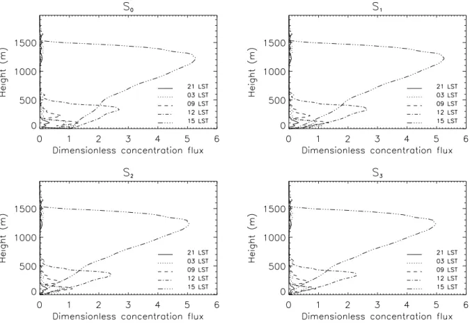
Fig. 5. Vertical profiles of S0and its progeny.
gradients are related to the concentration imbalance between the members of radon decaying family. Since218Po (S1) is
the first daughter of the family, its production by the decay of
S0is more important where the S0concentrations are higher,
i.e. close to the surface. Its radioactive decay proceeds at a faster rate than the mixing. Since mixing is very weak in the NBL, freshly created218Po is decaying before being trans-ported. As a result, its radioactive contribution is mostly act-ing close to the surface. The same process occurs for R2and
R3, although, due the slower decaying rates of (S2) and (S3),
the vertical gradients are not as strong as for R1.
6 Daytime turbulent dispersion
Figure 10 shows the daytime evolution of the concentration of 222Rn (S0) and the short-lived daughters S1, S2 and S3.
No fresh emissions of S0reach the reservoir layer resulting
from the previous day CBL and from the nocturnal BL since they are decoupled from the surface. Radon and its progeny concentrations decrease with time in the reservoir layer as result of the decaying process. In the CBL, similar concen-tration behaviors can be observed for S0and the daughters:
as the boundary layer deepens with time, the concentrations
decrease despite of fresh emission of radon at the surface and the production of the daughters through the decay chain. As mentioned previously, this behavior is the result of an imbal-ance between production by surface emissions and the de-caying chain on one hand, and dilution by boundary layer deepening and ventilation on the other. In order to under-stand the processes dominating the collapse of the222Rn and its short-lived daughters concentration during the morning transition of the convective boundary layer, we focus in the following on the vertical profiles of the fluxes (Fig. 11) and the radioactive decay contributions (Fig. 12).
The growth of the boundary layer is inducing ventilation at the top of the CBL. While the boundary layer is deepening, air masses with smaller concentrations are entrained from above. Turbulence transport is locally balancing the gradi-ent of concgradi-entration induced by the gradi-entrainmgradi-ent of cleaner air by transporting radionuclides from within the CBL to-wards it upper boundary (Fig. 11). This upward flux is more vigorous when the ventilation process is enhanced by the in-crease of the boundary layer growth rate. As a result we found important detrainment fluxes, i.e. positive flux values at the entrainment interface, that were even larger than the emission flux for S0 at the surface. Actually, two
5010 J.-F. Vinuesa et al.: Diurnal evolution of222Rn and its daughters
Fig. 6. Vertical profiles of the fluxes of S0and its progeny. The fluxes are made dimensionless by using the exhalation rate of radon.
figure: one at 10:00 LST and the one at around 12:30 LST. These maxima occur when the growth of the boundary layer depth, and therefore also the entrainment velocity we, shows
a maximum (see Fig. 13, discussed in Sect. 7). This confirms that the high flux values are due to the entrainment of low concentration air masses from above the CBL.
The radioactive decay term (Fig. 12) acts as a sink for
S0and as a source for its progeny. All contributions show
a maximum close to the surface, but with different vertical gradients: the gradient of R1 is extreme compared to those
of R2and R3, which show almost well-mixed profiles in the
lower-CBL and a maximum contribution at the bottom of the entrainment layer. This behavior was already mentioned by Vinuesa and Galmarini (2007) that attributed it to the inabil-ity of turbulence to mix efficiently radon short-lived daugh-ters that have a decaying temporal scale comparable to the turnover time of the CBL. Our findings confirm their analy-sis for a more realistic simulation.
7 Focusing on the mixed-layer characteristics
Figure 13 shows the evolution of the convective boundary layer growth focusing on the boundary layer depth zidefined
as the height where the minimum sensible heat flux is found,
the entrainment velocity we that is the speed of the
bound-ary layer growth, i.e. dzi
dt and the ratio of entrainment to the
surface flux of potential temperature βθ. From this figure,
three periods can be distinguished related to the character-istics of the unsteady growth of the CBL. After sunrise, the convective boundary layer starts to develop overlayed by the stable nocturnal boundary layer. At the top of it, the strong capping inversion is preventing thermals to develop. As a result, the boundary layer growth is slow but increasing as the CBL deepens. At around 10:00 LST, the boundary layer top reaches the maximum extension of the previous noctur-nal boundary layer. Due to the increase of the capping in-version at this interfacial layer (between the residual of the previous nocturnal boundary layer and the previous day con-vective boundary layer) the growth is slow down. Then the boundary layer continues to develop but now overlayed by the residual layer of the previous day CBL. The temperature jump at the top of the CBL is lower than previously (see also Fig. 1) and the growth is enhanced due to small temperature gradients across the entrainment zone. The boundary layer doubles its vertical extension within a few hours. At around 12:30 LST, the top of the CBL reaches the free troposphere. The strong capping inversion limits its development, the en-trainment velocity dramatically collapse and the CBL depth
Fig. 7. Time-height plots of the radon and its short-lived daughter concentrations. The boundary layer depth is shown using a solid line. It is
defined as the height where the turbulent heat flux is 5% of its surface value (Estournel and Guedalia, 1985).
is evolving toward a steady-state. The sharpness of the peak of entrainment velocity located at around 12:30 LST reflects the strength of the inversion.
Actually these periods are much more distinguishable while focusing on the mixed-layer concentrations of222Rn and its progeny i.e. <Si> and the ratio of entrainment to the
surface flux of222Rn β0=−(ws(ws0)e
0)s where (ws0)eand (ws0)s
are the entrainment and surface flux of S0, respectively. The
<Si> and β0are shown in Fig. 14
– To 09:30 LST: Initialization of convection, a sharp mixed-layer starts to develop overlayed by a strong stratification.
– From 09:30 to 11:00 LST: The mixed-layer is develop-ing within the leftover of the stable nocturnal bound-ary layer. <Si> decrease due to the entrainment of
less radon-concentrated air masses at the top of the CBL. This decrease is limited since air masses above the mixed layer contains Si that has been trapped
dur-ing the night.
– From 11:00 to 12:30 LST: The mixed-layer is develop-ing overlayed by the residual layer and <Si> collapse.
During the night, the reservoir layer has been almost de-coupled from the surface due to the stable stratification
of the nocturnal boundary layer. Since no fresh radon reached this layer, the radon short-lived daughter mix-ture aged and the system evolved toward secular equi-librium. Si is less abundant is the reservoir layer than
in the leftover of nocturnal boundary layer. Therefore, ventilation is entraining cleaner radon air masses than during the previous period and the decrease of <Si> is
more important.
– From 12:30 LST: The mixed-layer top has reached the free troposphere. The ventilation process still occurs but it is less important due to the collapse of weand the
low concentration gradient at the entrainment interface. The retrieval of the mixed-layer secular equilibrium is facilitated by the entrainment of radon and daughters mixture already in equilibrium.
When the CBL top reaches the free troposphere, large β0
values persist despite the decline in the entrainment velocity. These large values are due to the large gradient encountered in that region. When β0values are large, we found
appre-ciable S0 gradients within the mixed layer itself, due to the
CBL turnover mixing process. This is clearly shown by the 12:00 LST’s the profile of radon in Fig. 5. The same feature is also shown in Fig. 4 whenever β0is large in magnitude.
5012 J.-F. Vinuesa et al.: Diurnal evolution of222Rn and its daughters
Fig. 8. Time-height plots of the radon and its short-lived daughter dimensionless fluxes. The fluxes have been made dimensionless using
their maximum values. The boundary layer depth is shown using a solid line. It is defined as the height where the turbulent heat flux is 5% of its surface value (Estournel and Guedalia, 1985). The areas in white represents downward fluxes. The localisation of the maximum fluxes is shown in dashed lines.
Fig. 9. Time-height plots of the radioactive decay contributions Ri. The contributions have been made dimensionless using their maximum
values. The boundary layer depth is shown using a solid line. It is defined as the height where the turbulent heat flux is 5% of its surface value (Estournel and Guedalia, 1985).
Fig. 10. Time-height plots of the radon and its short-lived daughter concentrations. The daytime boundary layer depth, defined as the altitude
where the sensible heat flux is minimum, is also shown using solid white lines.
Fig. 11. Time-height plots of the radon and its short-lived daughter dimensionless fluxes.The fluxes have been made dimensionless using
their maximum values. The daytime boundary layer depth, defined as the altitude where the sensible heat flux is minimum, is also shown using a solid line.
5014 J.-F. Vinuesa et al.: Diurnal evolution of222Rn and its daughters
Fig. 12. Time-height plots of the radioactive decay −R0, R1, R2and R3. The contributions have been made dimensionless using their maximum values. The daytime boundary layer depth, defined as the altitude where the sensible heat flux is minimum, is also shown using solid white lines.
potential for the use of radon measurements as a delineator of CBL entrainment.
8 Secular equilibrium
If the radon daughters were subject only to the laws of ra-dioactive decay, the secular equilibrium imposed in the ini-tial activity profiles would be conserved along the simulation. However, departures from the equilibrium can be noticed in Fig. 15 that shows the radon and its short-lived daughters activity ratios. This disequilibrium is more important under stable stratification in the nocturnal boundary layer. Under convective conditions, the ratios evolve toward the equilib-rium value of 1.0 that is retrieved after the morning transi-tion. At the end of the day, the surface cooling results in a temperature stable stratification and in the formation of a thin boundary layer isolating the surface from the upper at-mosphere layer. In this stable layer, turbulence decays and departures from the equilibrium occur. It is interesting to no-tice that the equilibrium reached in the mixed layer of the previous day is preserved in the reservoir layer.
There has been extensive measurements of the disequilib-rium ratios in the surface layer for various type of stabili-ties (e.g., Beck and Gogolak, 1979; Hosler and Lockhart, 1965; Hosler, 1966). The largest departures from the sec-ular equilibrium were reported under stable conditions. The disequilibrium ratio was found to be also dependent on both the distance from the surface and the duration of the
stabil-ity regime. Quite a number of one-dimensional models have been formulated to relate the vertical distribution of the ra-dionuclide to the eddy diffusivity and to the exhalation rate of radon (e.g., Jacobi and Andre, 1963; Staley, 1966) and reached the same conclusions.
Several studies in the past have tried to correlate the stabil-ity regime with S0or the disequilibrium activity ratio.
How-ever, even if at first glance it appears that the equilibrium levels might be correlated directly with stability regime in the surface layer, the results shown in Fig. 16 reveal that other boundary layer characteristics are also influential. A given air parcel can be considered as a mixture of radon and its short-lived daughters. At sunset, if this parcel is close to the emission source of radon, it is composed of more freshly emitted radon than “old” radon. Because of the slow decay of radon, this air parcel contains more radon than its short-lived daughters. As a result, radon and its short-short-lived daugh-ters activity ratios are lower than 1. Throughout the night, the proportion of aging radon trapped in the stable boundary layer tends to increase (compared to “fresh” radon) and the mixture is evolving toward equilibrium. However, since the radioactive half-life of222Rn is 3.8 days, the night is obvi-ously not long enough to enable the secular equilibrium to be fully established. In Fig. 16, one can notice that the ac-tivity ratios collapse in the evening and increase during the night.
During the convective daytime period, turbulent eddy mo-tions are mixing the radon being exhaled from the soil into
Fig. 13. Boundary layer depth zi, entrainment velocity we and
βθ time evolutions. Smoothed results are also shown in thick solid
lines.
aged radon mixture. Due to the mixing and the short turnover time, any air parcel of the CBL contains the same amount of “fresh” radon and “old” radon. Turbulent transport enables the radioactive system to evolve toward the equilibrium. As a result, after the morning transition the equilibrium is reached and the homogeneous composition of the radon and short-lived daughter mixture is maintained by the turnover of the CBL. Figure 16 shows important increases of the activity
ra-Fig. 14. Mixed layer concentrations <Si> and β0time evolution.
S0, S1, S2, and S3are represented in solid, dotted, dashed and
dot-dashed lines, respectively. Smoothed results are also shown in thick lines.
tio during the morning transition. Most of all, our results shows that the activity ratio between radon and its progeny cannot be used solely as an indicator of atmospheric stability for diurnal evolving ABL. As one can clearly see in Fig. 16 two values of the ratio correspond to the same stability value. In this figure, one can notice important differences in the de-parture from secular equilibrium at dusk between the ratios for different daughters. During the initiation of the stable nocturnal boundary layer, the change of S1/S0activity ratio
is rather small while the one of S3/S0can reach 4%. It is of
interest to consider wheter the driving process of these dif-ferences is mixing by nocturnal turbulence or aging of the radionuclide mixture. An appropriate number to investigate the effect of turbulence on the radionuclei is the Damk¨ohler number (Vinuesa and Galmarini, 2007), Dat defined as the
ratio between the integral time-scale of turbulent (τt) and the
chemical time-scale (τc). In Fig. 17, the Damk¨ohler
num-bers Dat for Radon and its short-lived daughters are plotted
against Obukhov length. Here, we use τt=zi/w∗for the
5016 J.-F. Vinuesa et al.: Diurnal evolution of222Rn and its daughters
Fig. 15. Radon and its short-lived daughters activity ratio versus
time-height.
and h are defined as the altitude where the sensible heat flux is minimum and where the turbulent heat flux is 5% of its surface value (Estournel and Guedalia, 1985), respectively. For the radionuclides, τc=λ−1j with j =0, 1, 2, 3 meaning
that the Damk¨ohler numbers differ by the radioactive decay-ing rates. Therefore S1 and S2 are the daughters most and
least (respectively) affected by turbulence in Fig. 17. How-ever, the most important departure for secular equilibrium is found for S3in Fig. 16. This figure clearly shows that
noc-turnal turbulence does not have the dominant impact on the departure from secular equilibrium at dusk and, as mentioned previously, the driving process is the aging of the mixture of radon and short-lived daughters.
Fig. 16. Radon and its short-lived daughters activity ratio versus
Obukhov length at a height of 12.5 m above ground.
9 Conclusions
Numerical experiments were carried out using the state-of-the-art large-eddy simulation together with a new-generation subgrid-scale model to study the diurnal evolution of222Rn and its progeny in the atmospheric boundary layer. An ob-served diurnal cycle was successfully simulated and for the first time, the simulation included first-order decaying sys-tem represented by the the decaying chain of the222Rn fam-ily. By focusing our analysis on the night 33–34 and day 34 of the Wangara experiment, e.g. using the simulation of day 33 as a pre-run, and initializing the 222Rn and short-lived daughters’ concentrations as in a secular equilibrium,
Fig. 17. Radon and its short-lived daughters Damk¨ohler numbers versus Obukhov length. we were able to reproduce the realistic diurnal evolution of
the222Rn decaying family.
Near the surface, radon concentrations increase during the nocturnal stable period, reaching a maximum near sunrise. Following the breakup of a nocturnal surface-based radiation-type inversion, radon concentrations de-crease rapidly, reaching a minimum during the afternoon convective period.
A departure from secular equilibrium between radon and its short-lived daughter products prevails in the stable noc-turnal boundary layer. This disequilibrium is attributed to the proximity of the radon source and the weak vertical transport. Since a significant fraction of the radon is fresh, the radon and progeny mixture is deficient in daughters. The mixing induced by convective turbulence induces a fast restoration of the secular equilibrium during the morning transition.
Both turbulent transport and transport asymmetry of the
222Rn daily evolution are important consequence of the
en-trainment of “clean” air from the reservoir layers above into the boundary layer during its unsteady morning growth pe-riod. These entrainment events are responsible for the col-lapse of the mixed layer concentrations. Our analysis reveals that the spatial and temporal evolution of the concentrations of radon and its daughters is directly related to radioactive decay contribution in which turbulent mixing plays the major role. Thus, turbulent transport affect the dispersion of222Rn and its progeny by acting preferentially on the radioactive decay.
Acknowledgements. Computational resources were kindly
pro-vided by the High Performance Computing Center at the Texas Tech University.
Edited by: M. Ammann
References
Albertson, J. D. and Parlange, M. B.: Natural integration of scalar fluxes from complex terrain, Adv. Wat. Res., 23, 239–252, 1999. Anderson, W., Basu, S., and Letchford, C.: Comparison of dynamic subgrid-scale models for simulations of neutrally buoyant shear-driven atmospheric boundary layer flows, Env. Fluid Mech., 7, 195–215, 2007.
Andr´en, A., Brown, A. R., Graf, J., Mason, P. J., Moeng, C.-H., Nieuwstadt, F. T. M., and Schumann, U.: Large-eddy simulation of a neutrally stratified boundary layer: A comparison of four computer codes, Q. J. Roy. Meteor. Soc., 120, 1457–1484, 1994. Andr´en, A.: The structure of stably stratified atmospheric boundary layers: a large-eddy simulation study, Q. J. Roy. Meteor. Soc., 121, 961–985, 1995.
Basu, S. and Port´e-Agel, F.: Large-eddy simulation of stably strati-fied atmospheric boundary layer turbulence: a scale-dependent dynamic modeling approach, J. Atmos. Sci., 63, 2074–2091, 2006.
Basu, S., Port´e-Agel, F., Foufoula-Georgiou, E., Vinuesa, J.-F., and Pahlow, M.: Revisiting the local scaling hypothesis in stably stratified atmospheric boundary-layer turbulence: an integration of field and laboratory measurements with large-eddy simula-tions, Boundary-Layer Meteorol., 119, 473–500, 2006.
Basu, S., Vinuesa, J.-F., and Swift, A.: Dynamic LES modeling of a diurnal cycle, J. Appl. Meteorol. Clim., in press, 2007. Beare, R. J., Macvean, M. K., Holtslag, A. A. M., Cuxart, J., Esau,
I., Golaz, J.-C., Jimenez, M. A., Khairoutdinov, M., Kosovic, B, Lewellen, D., Lund, T. S., Lundquist, J. K., Mccabe, A., Moene, A. F., Noh, Y., Raasch, S., and Sullivan, P.: An
intercom-5018 J.-F. Vinuesa et al.: Diurnal evolution of222Rn and its daughters
parison of large-eddy simulations of the stable boundary layer, Boundary-Layer Meteorol., 118, 247–272, 2006.
Beck, H. L. and Gogolak, C. V.: Time dependent calculation of the vertical distribution of 222Rn and its decay products in the atmosphere, J. Geophys. Res., 84, 3139–3148, 1979.
Bou-Zeid, E., Meneveau, C., and Parlange, M.: A scale-dependent Lagrangian dynamic model for large eddy simula-tion of complex turbulent flows, Phys. Fluids, 17, 025105, doi:10.1063/1.1839152, 2005.
Brown, A. R., Derbyshire, S. H., and Mason, P. J.: Large-eddy simulation of stable atmospheric boundary layers with a revised stochastic subgrid model, Q. J. Roy. Meteor. Soc., 120, 1485– 1512, 1994.
Chow, F. K., Street, R. L., Xue, M., and Ferziger, J. H.: Explicit filtering and reconstruction turbulence modelingfor large-eddy simulation of neutral boundary layer flow, J. Atmos. Sci., 62, 2058–2077, 2005.
Clarke, R. H., Dyer, A. J., Brook, R. R., Reid, D. G., and Troup, A. J.: The Wangara experiment: boundary layer data, Paper No. 19, Div. Meteorol. Physics Aspendale, CSIRO, Australia, 362 pp., 1971.
Deardorff, J. W.: Preliminary results from numerical integrations of the unstable planetary boundary layer, J. Atmos. Sci., 27, 1209– 1211, 1970.
Deardorff, J. W.: Numerical investigation of neutral and unstable planetary boundary layers, J. Atmos. Sci., 29, 91–115, 1972. Deardorff, J. W.: Three-dimensional numerical study of the
height and mean structure of a heated planetary boundary layer, Boundary-Layer Meteorol., 7, 81–106, 1974a.
Deardorff, J. W.: Three-dimensional numerical study of turbulence in an entraining mixed layer, Boundary-Layer Meteorol., 7, 199– 226, 1974b.
Deardorff, J. W.: Stratocumulus-capped mixed layers derived from a three-dimensional model, Boundary-Layer Meteorol., 18, 495– 527, 1980.
Dentener, F., Feichter, J., and Jeuken, A.: Simulation of the trans-port of Rn-222 using on-line and off-line global models at differ-ent horizontal resolutions: a detailed comparison with measure-ments, Tellus, 51B, 573–602, 1999.
Esau, I.: Simulation of Ekman boundary layers by large eddy model with dynamic mixed subfilter closure, Environ. Fluid Mech., 4, 273–303, 2004.
Estournel, C. and Guedalia, D.: Influence of geostrophic wind on atmospheric nocturnal cooling, J. Atmos. Sci., 42, 2695-2698, 1985.
Galmarini, S.: One year of 222-Rn concentration in the atmospheric surface layer, Atmos. Chem. Phys. 6, 2865–2887, 2006. Genthon, C. and Armengaud, A.: Radon-222 as a comparative
tracer of transport and mixing in 2 general-circulation models of the atmosphere, J. Geophys. Res., 100, 2849–2866, 1995. Hess, G. D., Hicks, B. B., and Yamada, T.: The impact of the
Wan-gara experiment, Boundary-Layer Meteorol., 20, 135–174, 1981. Hicks, B. B.: An analysis of Wangara micrometeorology: surface stress, sensible heat, evaporation, and dewfall. Air Resources Laboratories, Silver Spring, Maryland, Tech. Rep. NOAA Tech-nical Memorandum ERL ARL-104, 36 pp., 1981.
Hosler, C. R. and Lockhart, L. B.: Simultaneous measurment of
222Rn,214Pb and214Bi in air near the ground, J. Geophys. Res.,
70, 4537–4546, 1965.
Hosler, C. R.: Meteorological effects on atmospheric concentra-tions of Radon (Rn222), RaB (Pb214), and RaC (Bi214) near the ground, Mon. Weather Rev., 94, 89–99, 1966.
Jacob, D. J., Prather, M. J., Rasch, P. J., Shia, R. L., Balkanski, Y. J., Beagley, S. R., Bergmann, D. J., Blackshear, W. T., Brown, M., Chiba, M., Chipperfield, M. P., deGrandpre, J., Dignon, J. E., Feichter, J., Genthon, C., Grose, W. L., Kasibhatla, P. S., Kohler, I., Kritz, M. A., Law, K., Penner, J. E., Ramonet, M., Reeves, C. E., Rotman, D. A., Stockwell, D. Z., VanVelthoven, P. F. J., Verver, G., Wild, O., Yang, H., and Zimmermann, P.: Evaluation and intercomparison of global atmospheric transport models using Rn-222 and other short-lived tracers, J. Geophys. Res., 102, 5953–5970, 1997.
Jacobi, W. and Andre, K.: The vertical distribution of 222Rn, 220Rn and their decay products in the atmosphere, J. Geophys. Res., 68, 3799–3814, 1963.
Khanna, S. and Brasseur, J. G.: Analysis of Monin-Obukhov simi-larity from large-eddy simulation, J. Fluid Mech., 345, 251–286, 1997.
Kumar, V., Kleissl, J., Meneveau, C., and Parlange, M. B.: Large-eddy simulation of a diurnal cycle of the atmospheric boundary layer: Atmospheric stability and scaling issues, Water Resour. Res., 42, W06D09, doi:10.1029/2005WR004651, 2006. Kosovi´c, B.: Subgrid-scale modelling for the large-eddy simulation
of high-Reynolds-number boundary layers, J. Fluid Mech., 338, 151–182, 1997.
Kosovi´c, B. and Curry, J. A.: A large eddy simulation study of a quasi-steady, stably stratified atmospheric boundary layer, J. At-mos. Sci., 57, 1052–1068, 2000.
Lewellen, D. C. and Lewellen, W. S.: Large-eddy boundary layer entrainment, J. Atmos. Sci., 55, 2645–2665, 1998.
Li, Y. H. and Chang, J. S.: A three-dimensional global episodic tracer transport model. 1. Evaluation of its processes by radon 222 simulations, J. Geophys. Res., 101, 25 931–25 947, 1996. Lin, C.-L., McWilliams, J. C., Moeng, C.-H., and Sullivan, P. P.:
Coherent structures and dynamics in a neutrally stratified plane-tary boundary layer flow, Phys. Fluids, 8, 2626–2639, 1996. Mason, P. J. and Thomson, D. J.: Large-eddy simulations of the
neutral-static-stability planetary boundary layer, Q. J. Roy. Me-teor. Soc., 113, 413–443, 1987.
Mason, P. J.: Large-eddy Simulation of the Convective Atmospheric Boundary Layer, J. Atmos. Sci., 46, 1492–1516, 1989.
Mason, P. J. and Derbysire, S. H.: Large-eddy simulation of the stably-stratified atmospheric boundary layer, Boundary-Layer Meteorol., 53, 117–162, 1990.
Moeng, C. H. and Wyngaard, J. C.: Statistics of conservative scalars in the convective boundary layer, J. Atmos. Sci., 41, 3161–3169, 1984.
Moeng, C. H. and Sullivan, P. P.: A comparison of shear- and buoyancy-driven planetary boundary layer flows, J. Atmos. Sci., 51, 999–1022, 1994.
Nieuwstadt, F. T. M., Mason, P. J., Moeng, C.-H., and Schumann, U.: Large-eddy simulation of the convective boundary layer: a comparison of four computer codes, in: Turbulent Shear Flows 8, edited by: Durst, F., Friedrich, R., Launder, B. E., Schmidt, F. W., Schumann, U., and Whitelaw, J. H., Springer, 347–367, 1991.
Port´e-Agel, F., Meneveau, C., and Parlange, M. B.: A scale-dependent dynamic model for large-eddy simulations:
applica-tion to a neutral atmospheric boundary layer, J. Fluid Mech., 415, 261–284, 2000.
Port´e-Agel, F.: A scale dependent dynamic model for scalar trans-port in LES of the atmospheric boundary layer, Bound.-Layer Meteorol., 112, 81–105, 2004.
Saiki, E. M., Moeng, C.-H., and Sullivan, P. P.: Large-eddy simula-tion of the stably stratified planetary boundary layer, Boundary-Layer Meteorol., 95, 1–30, 2000.
Schumann, U.: Large-eddy simulation of turbulent diffusion with chemical reactions in the convective boundary layer, Atmos. En-viron., 23, 1713–1729, 1989.
Staley, D. O.: The diurnal oscillations of radon and thoron and their decay products, J. Geophys. Res., 71, 3357–3367, 1966. Stoll, R., and Port´e-Agel, F.: Dynamic subgrid-scale
mod-els for momentum and scalar fluxes in large-eddy simula-tions of neutrally stratified atmospheric boundary layers over heterogeneous terrain, Water. Resour. Res., 42, W01409, doi:10.1029/2005WR003989, 2006.
Sullivan, P. P., Moeng, C.-H., Stevens, B., Lenschow, D. H., and Mayor, S. D.: Structure of the entrainment zone capping the con-vective atmospheric boundary layer, J. Atmos. Sci., 55, 3042– 3064, 1998.
Sykes, R. I. and Henn, D. S.: Large-eddy simulation of turbulent sheared convection, J. Atmos. Sci., 46, 1106–1118, 1989. UNSCEAR: Sources and effects of ionizing radiation. Volume
1: sources. United Nations Scientific Committee on Effects of Atomic Radiation, UN publication, New York, 2000.
Vinuesa, J.-F. and Port´e-Agel, F.: A dynamic similarity sub-grid model for chemical transformations in LES of the at-mospheric boundary layer, Geophys. Res. Lett., 32, L03814, doi:10.1029/2004GL021349, 2005.
Vinuesa, J.-F. and Galmarini, S.: Characterization of the222Rn fam-ily turbulent transport in the convective atmospheric boundary layer, Atmos. Chem. Phys., 7, 697–712, 2007,
http://www.atmos-chem-phys.net/7/697/2007/.
Yamada, T. and Mellor, G.: A simulation of the Wangara atmo-spheric boundary layer data, J. Atmos. Sci., 32, 2309–2329, 1975.