HAL Id: hal-01185927
https://hal.inria.fr/hal-01185927
Submitted on 25 Aug 2015HAL is a multi-disciplinary open access
archive for the deposit and dissemination of sci-entific research documents, whether they are pub-lished or not. The documents may come from teaching and research institutions in France or abroad, or from public or private research centers.
L’archive ouverte pluridisciplinaire HAL, est destinée au dépôt et à la diffusion de documents scientifiques de niveau recherche, publiés ou non, émanant des établissements d’enseignement et de recherche français ou étrangers, des laboratoires publics ou privés.
Comparing Word Representations for Implicit Discourse
Relation Classification
Chloé Braud, Pascal Denis
To cite this version:
Chloé Braud, Pascal Denis. Comparing Word Representations for Implicit Discourse Relation Clas-sification. Empirical Methods in Natural Language Processing (EMNLP 2015), Sep 2015, Lisbonne, Portugal. �hal-01185927�
Comparing Word Representations for
Implicit Discourse Relation Classification
Chlo´e Braud
ALPAGE, Univ Paris Diderot & INRIA Paris-Rocquencourt
75013 Paris - France [email protected]
Pascal Denis
MAGNET, INRIA Lille Nord-Europe 59650 Villeneuve d’Ascq - France
Abstract
This paper presents a detailed compar-ative framework for assessing the use-fulness of unsupervised word representa-tions for identifying so-called implicit dis-course relations. Specifically, we compare standard one-hot word pair representations against low-dimensional ones based on Brown clusters and word embeddings. We also consider various word vector combi-nation schemes for deriving discourse seg-ment representations from word vectors, and compare representations based either on all words or limited to head words. Our main finding is that denser represen-tations systematically outperform sparser ones and give state-of-the-art performance or above without the need for additional hand-crafted features.
1 Introduction
Identifying discourse relations is an important task, either to build a discourse parser or to help other NLP systems such as text summarization or question-answering. This task is relatively straightforward when a discourse connective, such as but or because, is used (Pitler and Nenkova, 2009). The identification becomes much more challenging when such an overt marker is lacking, and the relation needs to be inferred through other means. In (1), the presence of the pair of verbs (rose,tumbled) triggers a Contrast relation. Such relations are extremely pervasive in real text cor-pora: they account for about 50% of all relations in the Penn Discourse Treebank (Prasad et al., 2008). (1) [ Quarterly revenue rose 4.5%, to $2.3 billion from $2.2 billion]arg1 [ For the year, net
in-come tumbled 61% to $86 million, or $1.55 a share]arg2
Automatically classifying implicit relations is dif-ficult in large part because it relies on numerous factors, ranging from syntax, and tense and as-pect, to lexical semantics and even world knowl-edge (Asher and Lascarides, 2003). Consequently, a lot of previous work on this problem have at-tempted to incorporate some of these information into their systems. These assume the existence of syntactic parsers and lexical databases of var-ious kinds, which are available but for a few lan-guages, and they often involve heavy feature en-gineering (Pitler et al., 2009; Park and Cardie, 2012). While acknowledging this knowledge bot-tleneck, this paper focuses on trying to predict im-plicit relations based on easily accessible lexical features, targeting in particular simple word-based features, such as pairs like (rose,tumbled) in (1). Most previous studies on implicit relations, go-ing back to (Marcu and Echihabi, 2002), in-corporate word-based information in the form of word pair features defined across the pair of text segments to be related. Such word pairs are often encoded in a one-hot represen-tation, in which each possible word pair corre-sponds to a single component of a very high-dimensional vector. From a machine learning perspective, this type of sparse representation makes parameter estimation extremely difficult and prone to overfitting. It also makes it diffi-cult to achieve any interesting semantic general-ization. To see this, consider the distance (e.g., Euclidean or cosine) induced by such representa-tion. Assuming for simplicity that one character-izes each pair of discourse segments via their main verbs, the corresponding one-hot encoding for the pair (rose,tumbled) would be at equal distance from the synonymic pair (went up,lost) and the antonymic pair (went down,gained), as all three vectors are orthogonal to each others.
Various attempts have been made at reducing sparsity of lexical features. Recently,
Ruther-ford and Xue (2014) proposed to use Brown clus-ters (Brown et al., 1992) for this task, in effect replacing each token by its cluster binary code. These authors conclude that these denser, cluster-derived representations significantly improve the identification of implicit discourse relations and report the best performance to date using also additional features. Unfortunately, their claim is somewhat weakened by the fact that they fail to compare the use of their cluster word pairs against other types of word representations, in-cluding one-hot encodings of word pairs or other low-dimensional word representations. This work also leaves other important questions open. In par-ticular, it is unclear whether all word pairs con-structed over the two discourse segments are truly informative and should be included in the model. Given that word embeddings capture latent syn-tactic and semantic information, yet another im-portant question is to which extent the use of these representations dispenses us from using additional hand-crafted syntactic and semantic features.
This paper fills these gaps and significantly ex-tends the work of (Rutherford and Xue, 2014) by explicitly comparing various types of word representations and vector composition meth-ods. Specifically, we investigate three well-known word embeddings, namely Collobert and We-ston (Collobert and WeWe-ston, 2008), hierarchical log-bilinear model (Mnih and Hinton, 2007) and Hellinger Principal Component Analysis (Lebret and Collobert, 2014), in addition to Brown cluster-based and standard one-hot representations. All these word representations are publicly available for English and can be easily acquired for other languages just using raw text data, thus alleviat-ing the need for hand-crafted lexical databases. This makes our approach easily extendable to resource-poor languages. In addition, we also in-vestigate the issue of which specific words need to be fed to the model, by comparing using just pairs of verbs against all pairs of words, and how word representations should be combined over discourse segments, comparing component-wise product against simple vector concatenation.
2 Word Representations
A word representation associates a word to a math-ematical object, typically a high-dimensional vec-tor in {0, 1}|V|or R|V|, where V is a base vocabu-lary. Each dimension of this vector corresponds to
a feature which might have a syntactic or semantic interpretation. In the following, we review differ-ent types of word represdiffer-entations used in NLP. 2.1 One-hot Word Representations
Given a particular NLP problem, the crudest and yet most common type of word representation consists in mapping each word into a one-hot vec-tor, wherein each observed word corresponds to a distinct vector component. More formally, let V denote the set of all words found in the texts and w a particular word in V. The one-hot represen-tation of w is the d-dimensional indicator vector, noted 1w, such that d = |V|: that is, all of this
vector’s components are 0’s but for one 1 compo-nent corresponding to the word’s index in V. It is easy to see that this representation is extremely sparse, and makes learning difficult as it mechani-cally blows up the parameter space of the model. 2.2 Clustering-based Word Representations An alternative to these very sparse representations consists in learning word representations in an un-supervised fashion using clustering. An example of this approach are the so-called Brown clusters induced using the Brown hierarchical clustering algorithm (Brown et al., 1992) with the goal of maximizing the mutual information of bigrams. As a result, each word is associated to a binary code corresponding to the cluster it belongs to. Given the hierarchical nature of the algorithm, one can create word classes of different levels of granularity, corresponding to bit codes of different sizes. The less clusters, the less fine-grained the distinctions between words but the less sparsity. Note that this kind of representations also yields one-hot encodings but on a much smaller vocab-ulary size (i.e., the number of clusters). Brown clusters have been used for several NLP tasks, in-cluding NER, chunking (Turian et al., 2010), pars-ing (Koo et al., 2008) and implicit discourse rela-tion classificarela-tion (Rutherford and Xue, 2014). 2.3 Dense Real-Valued Representations Another approach to induce word representations from raw text is to learn distributed word represen-tations (aka word embeddings), which are dense, low-dimensional, and real-valued vectors. These are typically learned using neural language models (Bengio et al., 2003). Each dimension correspond-ing to a latent feature of the word that captures paradigmatic information. An example of such
embeddings are the so-called Collobert and We-ston embeddings (Collobert and WeWe-ston, 2008). The embeddings are learned discriminatively by minimizing a loss between the current n-gram and a corrupted n-gram whose last word comes from the same vocabulary but is different from the last word of the original n-gram. Another example are the Hierarchical log-bilinear embeddings (Mnih and Hinton, 2007) induced using a probabilistic and linear neural model, with a hierarchical prin-ciple used to speed up the model evaluation. The embeddings are obtained by concatenating the em-beddings of the n−1 words of a n-gram and learn-ing the embeddlearn-ing of the last word.
A final approach is based on the assumption that words occurring in similar contexts tend to have similar meanings. Building word distribu-tional representations is done by computing the raw cooccurrence frequencies between each word and the |D| words that serve as context, with D generally smaller than the overall vocabulary, then applying some transformation (e.g. TF-IDF). As |D| is generally too large to form a tractable rep-resentation, a dimensionality reduction algorithm is used to end up with p |D| dimensions. Like for distributed representations, we end up with a dense low-dimensional real-valued vector for each word. A recent example of such approach is the Hellinger PCA embeddings of (Lebret and Collobert, 2014) which were built using Principal Component Analysis based on Hellinger distance as dimensionality reduction algorithm. An impor-tant appeal of these representations is that they are much less time-consuming to train than the ones based on neural language models while allowing similar performance (Lebret and Collobert, 2014).
3 Segment Pair Representations
We now turn to the issue of combining the word representations as described in section 2 into com-posite vectors corresponding to implicit discourse classification instances. Schematically, the rep-resentations employed for pairs of discourse seg-ments differ along three main dimensions. First, we compare the use of a single word per segment (roughly, the two main verbs) against that of all the words contained in the two segments. Second, we compare the use of sparse (i.e., one-hot) vs. dense representations for words. As discussed, Brown cluster bit representations are a special (i.e., low-dimensional) version of one-hot encoding. Third,
we use two different types of combinations of word vectors to yield segment vector representa-tions: concatenation and Kronecker product. The proposed framework is therefore much more gen-eral than the one given in previous work such as (Rutherford and Xue, 2014).
3.1 Notation
Our classification inputs are pairs of text seg-ments, the two arguments of the relation to be pre-dicted. Let S1 = {w11, . . . , w1n} denote the n
words that make up the first segment and S2 =
{w21, . . . , w2m} the m words in the second
seg-ment. That is, we regard segments as bags of words. Let V again denote the word vocabulary, that is the set of all words found in the segments. Sometimes, we will find it useful to refer to a par-ticular subset of V. Let head(·) refer to the func-tion that extracts the head word of segment S,1and Vh ⊆ V the set of head words. As our goal is to compare different feature representations, we de-fine Φ as a generic feature function mapping pairs of segments to a d-dimensional real vector:
Φ : Vn× Vm→ Rd (S1, S2) 7→ Φ(S1, S2)
The goal of learning is to acquire for each relation a linear classification function fw(·), parametrized
by w ∈ Rd, mapping Φ(S1, S2) into {−1, +1}.
Recall that1wrefers to the d-dimensional
one-hot encoding for word w ∈ V. Let us also denote by ⊕ and ⊗ the vector concatenation operator and the Kronecker product, respectively. Note that do-ing a Kronecker product on two vectors u ∈ Rm and v ∈ Rnis equivalent to doing the outer prod-uct uv> ∈ Rm×n. Finally, the vec(·) operator
converts a m × n matrix into an mn × 1 column vector by stacking its columns.
3.2 Representations based on head words One of the simplest representation one can con-struct for a pair of segments (S1, S2) is to
con-sider only their head words: h1 = head(S1) and
h2 = head(S2). In this simple scenario, two
main questions that remain are: (i) which vector representations do we use for h1 and h2, and (ii)
how do we combine these representations. An im-portant criterion for word vector combination is that they retain text ordering information between text segments which really matters for this task.
Thus, inverting the order between two main verbs (e.g., push and fall) will often lead to distinct dis-course relation being inferred, as some relations are asymmetric (e.g., Result or Explanation). One-hot representations Starting again with the simplest case, one can use the one-hot encod-ings corresponding to the two head words,1h1 and
1h2 respectively, and combine them using either
concatenation or product, leading to our two first feature mappings:
Φh,1,⊕(S1, S2) =1h1⊕1h2
Φh,1,⊗(S1, S2) = vec(1h1⊗1h2)
Note that Φh,1,⊕(S1, S2) lives in {0, 1}2|Vh| and
Φh,1,⊗ in {0, 1}|Vh|
2
. The latter representation amounts to assigning one 1 component for each pair of words in Vh × Vh, and is the sparsest
representation one can construct from head words alone. In some sense, it is also the most expressive in that we learn one parameter for each word pair, hence capturing interaction between words across segments. By contrast, Φh,1,⊕(S1, S2) doesn’t
ex-plicitly model word interaction across discourse segments, treating each word in a given segment (left or right) as a separate dimension.
Dense representations Alternatively, one can represent head words through their real low-dimensional embeddings. Let M denote a n × p real matrix, wherein the ith row corresponds to the p-dimensional embedding of the ith word of Vh, with p |Vh|.2 Using this notation, one
can derive the word embeddings of the head words h1 and h2 from their one-hot representations
us-ing simple matrix multiplication: M>1h1 and
M>1h2, respectively. Concatenation and product
yield two new feature mappings, respectively: Φh,M ,⊕(S1, S2) = M>1h1 ⊕ M >1 h2 Φh,M ,⊗(S1, S2) = vec(M>1h1 ⊗ M >1 h2)
These new representations live in a much lower dimensional real spaces: Φh,M ,⊕(S1, S2) lives in
R2pand Φh,M ,⊗(S1, S2) in Rp
2
.
3.3 Representations based on all words The various segment-pair representations that we derived from pairs of head words can be general-ized to the case in which we keep all the words in
2For now, we assume that n = V
hwhich is unrealistic.
See section 4.1 for a discussion of unknown words.
each segment. The additional issue in this context is in the combination of the different word vec-tor representations within and across the two seg-ments, and that of normalizing the segment vec-tors thus obtained. For simplicity, we assume that the representation for each segment is computed by summing over the pairs of words vectors com-posing the segments.
One-hot representations Following this ap-proach and recalling that S1 contains n words,
while S2 has m words, one can construct one-hot
encodings for segment pairs as follows:
Φall,1,⊕(S1, S2) = n X i m X j 1w1i ⊕1w2j Φall,1,⊗(S1, S2) = n X i m X j vec(1w1i ⊗1w2j)
If used without any type of frequency thresh-olding, these mappings result in very high-dimensional feature representations living in Z2|V|≥0
and Z|V|≥02, respectively. Interestingly, note that
the feature mapping Φall,1,⊗(S1, S2) corresponds
to the standard segment-pair representation used in many previous work, as (Marcu and Echihabi, 2002; Park and Cardie, 2012).
Dense representations We can apply the same composition operations to denser representations, yielding two new mappings:
Φall,M ,⊕(S1, S2) = n,m X i,j M>1w1i ⊕ M>1w2j Φall,M ,⊗(S1, S2)= n,m X i,j vec(M>1w1i⊗M>1w2j)
Like their head word versions, these vectors live in R2pand Rp2, respectively.
Vector Normalization Normalization is impor-tant as unnormalized composite vectors are sen-sitive to the number of words present in the seg-ments. The first type of normalization we consider is to simply convert our vector representation into vectors on the unit hypersphere: this is achieved by dividing each vector by its L2norm.
Another type of normalization is obtained by in-verting the order of summation and concatenation in the construction of composite vectors. Instead
of summing over concatenated pairs of word vec-tors across the two segments, one can first sum in-dividual word vectors within each segment, then concatenate the two segment vectors. One can thus use mapping Φ0all,1,⊕in lieu of Φall,1,⊕:
Φ0all,1,⊕(S1, S2) = n X i 1w1i ⊕ m X j 1w2j
It should be clear that Φ0all,1,⊕ provides a nor-malized version of Φall,1,⊕as this latter mapping
amounts to weighted versions of the former:
Φall,1,⊕(S1, S2) = m n X i 1w1i ⊕ n m X j 1w2j 4 Experiment Settings
Through the comparative framework described in section 3, our objective is to assess the useful-ness of different vectorial representations for pairs of discourse segments. Specifically, we want to establish whether dense representations are better than sparse ones, and whether certain word pairs are more relevant than others, which resource and which combination schemes are more adapted to the task, and, finally, whether standard features de-rived from external databases are still relevant in the presence of dense representations.
4.1 Feature Set
Our main features are primarily lexical in nature and based on surface word forms. These are de-fined either on all words used in the relation argu-ments or only on their heads.
Head Extraction Heads of discourse segments are first extracted using Collins syntactic head rules3. In order to retrieve the semantic predi-cate, we define a heuristic which looks for the past participle of auxiliaries, the adjectival or nominal attribute of copula, the infinitive complementing ”have to” forms and the first head of coordination conjunctions. In case of multiple subtrees, we look for the head of the first independent clause, or, fail-ing that, of the first phrase.
Word Representations We use either one-hot encodings or use word embeddings to build denser representations as described in section 3. The Brown clusters (Brown), Collobert-Weston (CnW) representations, and the hierarchical log-bilinear
3https://github.com/jkkummerfeld/nlp-util
(HLBL) embeddings correspond to the versions implemented in (Turian et al., 2010)4. They have been built on Reuters English newswire with case left intact. We test versions with 100, 320, 1000 and 3, 200 clusters for Brown, with 25, 50, 100 and 200 dimensions for CnW and with 50 and 100 dimensions for HLBL. The Hellinger PCA (H-PCA) embeddings come from (Lebret and Col-lobert, 2014)5 and have been built over the en-tire English Wikipedia, the Reuters corpus and the Wall Street Journal with all words in lower case. The vocabulary corresponds to the words that ap-pear at least 100 times and normalized frequency is computed with the 10, 000 most frequent words as context words. We test versions with 50, 100 and 200 dimensions for H-PCA. The coverage of each resource is presented in table 1.
# words # missing words All words Head words
HLBL 246, 122 5, 439 171
CnW 268, 810 5, 638 171
Brown 247, 339 5, 413 171
H-PCA 178, 080 7, 042 190
Table 1: Word embeddings and Brown clusters lexicon coverage.
When presenting our results, we distinguish be-tween systems based on one-hot encoding built from raw tokens (one-hot) or Brown clusters (Brown). We group the systems that use embed-dings under Embed. When relevant, we indicate the number of dimensions (e.g. Brown 3,200 is the system using Brown clusters with 3, 200 clusters). We use the symbols defined in section 3 to repre-sent the operation linking the arguments represen-tations (e.g. one-hot ⊕ corresponds to the transfor-mation defined by Φh,1,⊕ when using heads and
by Φall,1,⊕when using all words).
Vocabulary Sizes For one-hot encoding, the case is left intact. We ignore the unknown words when using the Brown clusters following (Ruther-ford and Xue, 2014). For the word embeddings, we use the mean of the vectors of all words.
In order to give an idea of the sparsity of the one-hot encodings, note that we have |V| = 33, 649 different tokens considering all implicit examples without filtering. The Brown clusters
4
http://metaoptimize.com/projects/wordreprs/
merge these tokens into 3, 190 codes (for 3, 200 clusters), 393 (1, 000 clusters), 59 (320 clusters) or 16 (100 clusters). For heads, we count 5, 615 dif-ferent tokens which correspond to 1, 988 codes for 3, 200 clusters and roughly the same number for the others. For the dense representations, the vo-cabulary size is twice the number of dimensions of the embedding, thus from 50 to 400, or the square of this number, thus from 625 to 40, 000.
Other Features We experiment with additional features commonly used for this task: produc-tions rules, average verb phrases length, Levin verb classes, modality, polarity, General Inquirer tags, number, first last and first three words. These feature templates are well described in (Pitler et al., 2009; Park and Cardie, 2012). They all corre-spond to a one-hot encoding, except average verb phrases length which is continuous. We thus con-catenate these features to the lexical ones.
4.2 Model
We use the same classification algorithm for com-paring all the described feature configurations. Specifically, we train a Maximum Entropy (ME) classifier (aka, logistic regression).6 As in previ-ous studies, we build one binary classifier for each relation. In order to deal with class imbalance, we use a sample weighting scheme: each sample re-ceives a weight inversely proportional to the fre-quency of its class in the training set. We optimize the hyper-parameters of the algorithm (i.e., the regularization norm: L1 or L2, and its strength)
and a filter on the features on the development set, based on the F1 score. Note that filtering is point-less for purely dense representations. We test sta-tistical significancy of the results using t-test and Wilcoxon test on a split of the test set in 20 folds.
Previous studies have tested several algorithms generally concluding that Naive Bayes (NB) gives the best performance (Pitler et al., 2009; Ruther-ford and Xue, 2014). We found that, when the hyparameters of ME are well tuned, the per-formance are comparable to NB if not better. Note that NB cannot be used with word embed-dings representations as it does not handle neg-ative value. Concerning the class imbalance is-sue, the downsampling scheme is the most spread since (Pitler et al., 2009) but it has been shown
6We use the implementation provided in Scikit-Learn
(Pe-dregosa et al., 2011), available at: http://scikit-learn. org/dev/index.html.
that oversampling and instance weighting lead to better performance (Li and Nenkova, 2014a).
Relation Train Dev Test
Temporal 665 93 68
Contingency 3, 281 628 276
Comparison 1, 894 401 146
Expansion 6, 792 1, 253 556 Total 12, 632 2, 375 1, 046 Table 2: Number of examples in train, dev, test.
4.3 Penn Discourse Treebank
We use the Penn Discourse Treebank (Prasad et al., 2008), a corpus annotated at the discourse level upon the Penn Treebank, giving access to a gold syntactic annotation, and composed of arti-cles from the Wall Street Journal. Five types of examples are distinguished: implicit, explicit, al-ternative lexicalizations, entity relations, and no relation. Each example could carry multiple rela-tions, up to four for implicit ones, and the relations are organized into a three-level hierarchy.
We keep only true implicit examples and only the first annotation. We focus on the top level re-lations which correspond to general categories in-cluded in most discursive frameworks. Finally, in order to make comparison easier, we choose the most spread split of the data, used in (Pitler et al., 2009; Park and Cardie, 2012; Rutherford and Xue, 2014) among others. The amount of data for train-ing (sections 2 − 21), development (00, 01, 23, 24) and evaluation (21, 22) is summarized in table 2.
5 Results
We first discuss the models that use only lexical features, defined either over all the words that ap-pear in the arguments or only the head words. We then compare our best performing lexical configu-rations with the ones that also integrate additional standard features, and to state-of-the-art systems. 5.1 Word Pairs over the Arguments
Our first finding in this setting is that feature con-figurations that employ unsupervised word repre-sentations almost systematically outperform those that use raw tokens. This is shown in the left part of table 3. Although the optimal word rep-resentation differs from one relation to another, it is always a dense representation that achieves the
All words Head words only
Representation Temp. Cont. Compa. Exp. Temp. Cont. Compa. Exp.
One-hot⊗ 21.14 50.36 34.80 59.43 11.96 43.24 17.30 69.21 One-hot⊕ 23.04 51.31 34.06 58.96 23.01 49.40 29.23 59.08 Brown3, 200 ⊗ 20.38 50.95 34.85 61.23 11.98 43.77 16.75 68.76 Best Brown ⊗ 15.52 53.85∗∗ 30.90 61.87 22.91 45.74 25.83 68.76 Best Brown ⊕ 27.96∗∗ 49.48 31.19 67.42∗∗ 21.84 47.36 27.52 61.38 Best Embed. ⊗ 22.97 52.76∗∗ 34.99 61.87 23.88 51.29 30.59 58.59 Best Embed. ⊕ 25.98∗ 52.50 33.15 60.17 22.48 47.48 29.82 57.45
Table 3: F1 score for systems using all words and only heads for Temporal (Temp.), Contingency (Cont.), Comparison(Compa.) and Expansion (Exp.).∗p ≤ 0.1,∗∗p ≤ 0.05 compared to One-hot ⊗ with t-test and Wilcoxon ; for head words, all the improvements observed against One-hot ⊗ are significant.
best F1 score. Our baselines correspond to mul-tiplicative and additive one-hot encodings, noted One-hot⊗ and One-hot ⊕, the former being the most commonly used in previous work. These are strong baselines in the sense they have been ob-tained after optimizing a frequency cut-off. Our best systems based on dense representations corre-spond to significant improvements in terms of F1 of about 8 points for Expansion, 7 points for Tem-poraland 3.5 for Contingency. The gains for Com-parisonare not statistically significant. All these results are obtained using the normalization to unit vectors possibly combined to the concatenation-specific normalization described in §3.3.
Comparing Dense Representations The best results are obtained using the Brown clusters (Brown) showing that this resource merges words in a way that is relevant to the task. Strikingly, the Brown configuration used in (Rutherford and Xue, 2014) (One-hot Brown 3, 200 ⊗) does not do better than the raw word pair baselines, except for Expansion. Recall that these authors did not explicitly provide this comparison. While doing a little worse, word embeddings (Embed.) also yield significant improvements for Temporal and Contingency, and smaller improvements for the others. This suggests that, even if they were not built based on discursive criteria, the latent dimen-sions encode word properties that are relevant to their rhetorical function. The superiority of Brown clusters over word embeddings is in line with the conclusions in (Turian et al., 2010) for two rather different NLP tasks (i.e., NER and chunking).
Turian et al. (2010) showed that the optimal word embedding is task dependent. Our exper-iments suggest that it is relation dependent: the
best scores are obtained with HLBL for Tempo-ral, CnW for Contingency, H-PCA for Expansion and CnW (Best Embed. ⊗) and HPCA (Best Em-bed.⊕) for Comparison. This again demonstrates that these four relations have to be considered as four distinct tasks. Identifying temporal or causal links is indeed sensitive to very different factors, the former relying more on temporal expressions and temporal ordering of events whereas the lat-ter relies on lexical and encyclopaedic knowledge on events. We think that this also explains that the behavior of the F1 against the optimal number of clusters for Expansion really differs from what we observed for the other relations: only 100 clus-ters for the best concatenated system and 320 for the best multiplicative one. Expansion is the least semantically marked relation and thus takes less advantage of fine-grained semantic groupings.
Comparing Word Combinations Comparing concatenated configurations (⊕ systems) against multiplicative ones (⊗ systems), we first note that for raw tokens the concatenated form (one-hot ⊕) yields results that are comparable, and some-times better, than the standard multiplicative sys-tem (one-hot ⊗), while failing to explicitly model word pair interactions. With Brown clusters, the concatenated form Best Brown ⊕ lead to better F1 scores than Best Brown ⊗ except for Contingency. When comparing performance on dev set, we found that the differences between concatenated and multiplicative forms for Brown (excluding Ex-pansionfor now) depend on the number of clusters used. Turian et al. (2010) found that the more clus-ters, the better the performance. This is also the case here with concatenated forms, but not with multiplicative forms. In that case, F1 increases
un-til 1, 000 clusters and then decreases. There is in-deed a trade-off between expressivity and sparsity: having too few clusters means that we loose im-portant distinctions, but having too many clusters leads to a loss in generalization. A similar trend is also found with word embeddings.
5.2 Head Words Only
Considering the right part of table 3, the first find-ing is that performance of systems that use only head words decrease compared to those using all words, but much more so with the baseline One-hot ⊗ than with other representations. One-hot ⊗ has very poor performance for most relations, losing between 7 and 17 points in F1 score. The
performance loss is much less striking with One-hot⊕ and with denser representations, which are again the best performing. The only exception is Expansionwhose precision however increases. As said, this relation is the less semantically marked, making it less likely to take advantage of the use of word representations. The best performance in this setting are obtained with word embeddings (not Brown) with significant gain from 8 to 13 points in F1 for most relations. Moreover, the best systems are all based on the multiplicative form confirming that this is a better way of representing pairs than simple concatenation when the number of initial dimensions is not too large.
5.3 Adding Other Features
Finally, we would like to assess how much im-provement can still be obtained by adding other standard features, such as those in §4.1, to word-based features. Conversely, we want to evaluate how far we are from state-of-the-art performance by just using word representations. We compare our results with those presented in (Rutherford and Xue, 2014) and in (Ji and Eisenstein, 2014), both systems deal with sparsity either by using Brown clusters or by learning task-dependent representa-tions. To make comparison easier we reproduce the experiments in (Rutherford and Xue, 2014) with Naive Bayes (NB)7 and Maximum Entropy
(ME) but without their coreference features and using gold syntactic parse. These correspond to the “repr.” lines in table 4. We attribute the small differences observed with NB by the lack of coref-erence features and/or the use of different filter-ing thresholds. Concernfilter-ing the difference between
7Implemented in Scikit-Learn, we optimized the
hyper-parameter corresponding to the smoothing.
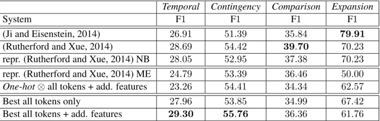
NB and ME, the only obvious issue is the low F1 score for Expansion: the system built using NB predicts all examples as positive thus leading to a high F1 score whereas the other one produces more balanced predictions, meaning neither sys-tems is truly satisfactory. Finally, we give results using the traditional one-encoding based on word pairs plus additional features (One-hot ⊗ + addi-tional features). These results are summarized in table 4, also including the best results of our ex-periments without additional features (“only”).
Our first finding is that the addition of extra features to our previous word-based only config-uration appears to outperform state-of-the art re-sults for Temporal and Contingency, thus giving the best performance to date on these relations. These improvements are significant compared to our reproduced systems. Note that we also out-perform the task-dependent embeddings of Ji and Eisenstein (2014), except for Expansion. Our ten-tative explanation for this is that these authors in-cluded Entity relations and coreference features. Note that our system corresponding to a reproduc-tion of (Rutherford and Xue, 2014) gives results similar to the baseline using raw word pairs (One-hot⊗ + additional features) showing that their im-provements were due to other factors, the opti-mized filter threshold and the coreference features. Overall, the addition of these hand-crafted fea-tures to our best systems do not provide improve-ments as high as one might have hoped. While improvements are significant compared to our re-produced systems, they are not with respect to the best systems given in table 3. When using all words, we only have a tendency toward significant improvement for Contingency8. These very small differences demonstrate that semantic and syntac-tic properties encoded in these features are already taken into account into the unsupervised word rep-resentations.
6 Related Work
Automatically identifying implicit relations is challenging due to the complex nature of the pre-dictors. Previous studies have thus used many fea-tures relying on several external resources (Pitler et al., 2009; Park and Cardie, 2012; Biran and McKeown, 2013) as the MPQA lexicon (Wilson et al., 2005) or the General Inquirer lexicon (Stone and Hunt, 1963), or on constituent or dependency
Temporal Contingency Comparison Expansion
System F1 F1 F1 F1
(Ji and Eisenstein, 2014) 26.91 51.39 35.84 79.91
(Rutherford and Xue, 2014) 28.69 54.42 39.70 70.23
repr. (Rutherford and Xue, 2014) NB 28.05 52.95 37.38 70.23
repr. (Rutherford and Xue, 2014) ME 24.79 53.39 36.46 50.00
One-hot⊗ all tokens + add. features 23.26 54.41 34.34 62.57
Best all tokens only 27.96 53.85 34.99 67.42
Best all tokens + add. features 29.30 55.76 36.36 61.76
Table 4: Systems using additional features (“+ add.features”), state-of-the art results either reported or reproduced (“repr.”) using Naive Bayes (“NB”) or logistic regression (“ME”) and best system from previous table (“only”).
parsers (Li and Nenkova, 2014b; Lin et al., 2009). Feature selection methods have been proved nec-essary to handle all of these features (Park and Cardie, 2012; Lin et al., 2009). Interestingly, Park and Cardie (2012) conclude on the worthlessness of word pair features, given the existence of such resources. We showed that provided unsupervised word representations, the opposite was in fact true, as dense word representations capture a lot of syn-tactic and semantic information.
The major problem of standard word pair repre-sentations is their sparsity. A line of work is to deal with this issue by adding automatically annotated data from explicit examples (Marcu and Echihabi, 2002), possibly using some kind of filtering or adaptation methods (Pitler et al., 2009; Biran and McKeown, 2013; Braud and Denis, 2014). An-other line of work propose to make use of dense representations as Brown clusters in (Rutherford and Xue, 2014). These authors claim that this re-source provides word representations that are rele-vant to the task, a conclusion that we considerably refined. Ji and Eisenstein (2014) propose to learn a distributed representation from the syntactic trees representing each argument in way that is more directly related to the task. Although this is an attractive idea, the score on top level PDTB rela-tions are mostly below those reported by (Ruther-ford and Xue, 2014), possibly because their repre-sentations are learned on a rather small corpus, the PDTB itself, whereas building this kind of repre-sentation requires massive amount of data.
Our work also relates to studies comparing un-supervised representations for other NLP tasks such as name entity recognition, chunking (Turian et al., 2010), sentiment analysis (Lebret and
Col-lobert, 2014) or POS tagging (Stratos and Collins, 2005). In particular, we found some similarities between our conclusions and those in (Turian et al., 2010). Our comparison is slightly richer in that it includes different methods of vector com-positions and add an extra distributional represen-tation to our comparison (namely, H-PCA).
7 Conclusions and Future Work
In this paper, we show that one can reach state-of-the-art results for implicit discourse relation iden-tification using only shallow lexical features and existing unsupervised word representations thus contradicting previous conclusions on the worth-lessness of these features. We carefully assess the usefulness of word representations for dis-course by comparing various formulations and combination schemes, demonstrating the inade-quacy of the previously proposed strategy based on Brown clusters and the distinctive relevance of head words, and by establishing that the created dense representations already provide most of the semantic and syntactic information relevant to the task thus alleviating the need for traditional exter-nal resources.
In future work, we first plan to extend our com-parative framework to a larger set of relations and to other languages. We also want to explore meth-ods for learning embeddings that are directly re-lated to the task of discourse relation classifica-tion, potentially using existing embeddings as ini-tialization (Labutov and Lipson, 2013). It is also clear that seeing discourse segments as bag of words is too simplistic, we would like to investi-gate ways of learning adequate segment-wide em-beddings.
References
N. Asher and A. Lascarides. 2003. Logics of Conver-sation. Cambridge University Press.
Yoshua Bengio, R´ejean Ducharme, Pascal Vincent, and Christian Janvin. 2003. A neural probabilistic lan-guage model. Journal of Machine Learning Re-search, 3:1137–1155.
Or Biran and Kathleen McKeown. 2013. Aggregated word pair features for implicit discourse relation dis-ambiguation. In Proceedings of the 51st Annual Meeting of the Association for Computational Lin-guistics.
Chlo´e Braud and Pascal Denis. 2014. Combining natural and artificial examples to improve implicit discourse relation identification. In Proceedings of the 25th International Conference on Computational Linguistics.
Peter F. Brown, Peter V. deSouza, Robert L. Mer-cer, Vincent J. Della Pietra, and Jenifer C. Lai. 1992. Class-based n-gram models of natural lan-guage. Computational Linguistics, 18:467–479. Ronan Collobert and Jason Weston. 2008. A unified
architecture for natural language processing: Deep neural networks with multitask learning. In Pro-ceedings of the 25th International Conference on Machine Learning.
Yangfeng Ji and Jacob Eisenstein. 2014. One vector is not enough: Entity-augmented distributional se-mantics for discourse relations. Transactions of the Association for Computational Linguistics.
Terry Koo, Xavier Carreras, and Michael Collins. 2008. Simple semi-supervised dependency parsing. In Proceedings of the 46th Annual Meeting of the Association for Computational Linguistics: Human Language Technologies.
Igor Labutov and Hod Lipson. 2013. Re-embedding words. In Proceedings of the 51th Annual Meeting of the Association for Computational Linguistics. R´emi Lebret and Ronan Collobert. 2014. Word
emdeddings through hellinger PCA. In Proceedings of the 14th Conference of the European Chapter of the Association for Computational Linguistics. Junyi Jessy Li and Ani Nenkova. 2014a. Addressing
class imbalance for improved recognition of implicit discourse relations. In Proceedings of the 15th An-nual Meeting of the Special Interest Group on Dis-course and Dialogue.
Junyi Jessy Li and Ani Nenkova. 2014b. Reducing sparsity improves the recognition of implicit dis-course relations. In Proceedings of the 15th Annual Meeting of the Special Interest Group on Discourse and Dialogue.
Ziheng Lin, Min-Yen Kan, and Hwee Tou Ng. 2009. Recognizing implicit discourse relations in the penn discourse treebank. In Proceedings of the 2009 Con-ference on Empirical Methods in Natural Language Processing.
Daniel Marcu and Abdessamad Echihabi. 2002. An unsupervised approach to recognizing discourse re-lations. In Proceedings of the 40th Annual Meeting on Association for Computational Linguistics. Andriy Mnih and Geoffrey Hinton. 2007. Three new
graphical models for statistical language modelling. In Proceedings of the 24th International Conference on Machine Learning.
Joonsuk Park and Claire Cardie. 2012. Improving im-plicit discourse relation recognition through feature set optimization. In Proceedings of the 13th Annual Meeting of the Special Interest Group on Discourse and Dialogue.
F. Pedregosa, G. Varoquaux, A. Gramfort, V. Michel, B. Thirion, O. Grisel, M. Blondel, P. Pretten-hofer, R. Weiss, V. Dubourg, J. Vanderplas, A. Pas-sos, D. Cournapeau, M. Brucher, M. Perrot, and E. Duchesnay. 2011. Scikit-learn: Machine learn-ing in Python. Journal of Machine Learnlearn-ing Re-search, 12:2825–2830.
Emily Pitler and Ani Nenkova. 2009. Using syntax to disambiguate explicit discourse connectives in text. In Proceedings of the 47th Annual Meeting of the Association for Computational Linguistics and the 4th International Joint Conference on Natural Lan-guage Processing of the AFNLP.
Emily Pitler, Annie Louis, and Ani Nenkova. 2009. Automatic sense prediction for implicit discourse re-lations in text. In Proceedings of the Joint Confer-ence of the 47th Annual Meeting of the ACL and the 4th International Joint Conference on Natural Lan-guage Processing of the AFNLP.
Rashmi Prasad, Nikhil Dinesh, Alan Lee, Eleni Milt-sakaki, Livio Robaldo, Aravind Joshi, and Bonnie Webber. 2008. The penn discourse treebank 2.0. In Proceedings of the Sixth International Conference on Language Resources and Evaluation.
Attapol Rutherford and Nianwen Xue. 2014. Dis-covering implicit discourse relations through brown cluster pair representation and coreference patterns. In Proceedings of the 14th Conference of the Euro-pean Chapter of the Association for Computational Linguistics.
Philip J. Stone and Earl B. Hunt. 1963. A computer approach to content analysis: Studies using the gen-eral inquirer system. In Proceedings of the Spring Joint Computer Conference.
Karl Stratos and Michael Collins. 2005. Simple semi-supervised pos tagging. In Proceedings of NAACL Workshop on Vector Space Modeling for NLP.
Joseph Turian, Lev-Arie Ratinov, and Yoshua Bengio. 2010. Word representations: A simple and general method for semi-supervised learning. In Proceed-ings of the 48th Annual Meeting of the Association for Computational Linguistics.
Theresa Wilson, Janyce Wiebe, and Paul Hoffmann. 2005. Recognizing contextual polarity in phrase-level sentiment analysis. In Proceedings of the Con-ference on Human Language Technology and Em-pirical Methods in Natural Language Processing.