A 64 channel 3T array coil for highly accelerated fetal imaging at 22 weeks of pregnancy

A 64 Channel 3T Array Coil for Highly Accelerated

Fetal Imaging at 22 Weeks of Pregnancy

by

Mark H. Spatz

Submitted to the Department of Electrical Engineering and Computer

Science

in partial fulfillment of the requirements for the degree of

Master of Engineering in Electrical Engineering and Computer Science

at the

MASSACHUSETTS INSTITUTE OF TECHNOLOGY

February 2017

c

○

Massachusetts Institute of Technology 2017. All rights reserved.

Author . . . .

Department of Electrical Engineering and Computer Science

Feb 3, 2017

Certified by. . . .

Lawrence L. Wald

Professor of Radiology, Harvard Medical School

Thesis Supervisor

Accepted by . . . .

Christopher Terman

Chairman, Masters of Engineering Thesis Committee

A 64 Channel 3T Array Coil for Highly Accelerated Fetal

Imaging at 22 Weeks of Pregnancy

by

Mark H. Spatz

Submitted to the Department of Electrical Engineering and Computer Science on Feb 3, 2017, in partial fulfillment of the

requirements for the degree of

Master of Engineering in Electrical Engineering and Computer Science

Abstract

MRI is an attractive tool for fetal imaging due to its unique ability to provide detailed anatomical and physiological data in an inherently safe manner. In practice, the problem of unpredictable and nonrigid fetal motion limits fetal MRI to fast single shot T2 weighted sequences such as HASTE, which have poor tissue contrast, low SNR, and cannot provide detailed physiological information. In this work, we designed, built, and tested a semi-adjustable anatomically shaped 64 channel array coil for fetal imaging at 22 weeks of pregnancy. The coil’s performance was compared to that of the vendor’s standard configuration consisting of an 18 channel flexible body array and 16 channels from a 32 channel spine array. The fetal coil provides roughly 5% better SNR in the fetal brain region of an anthropomorphic phantom and allows increasing SENSE acceleration factor from 𝑅 = 4 to 𝑅 = 5 in the right-left direction and 𝑅 = 3 to 𝑅 = 4 in the head-foot direction.

Thesis Supervisor: Lawrence L. Wald

Acknowledgments

I would like to thank, in order:

∙ My parents Jeff and Nancy, for catapulting me into a life wherein I’ve had the opportunity to pursue an advanced degree at MIT.

∙ My elementary, middle, and high school teachers.

∙ Larry Wald and Elfar Adalsteinsson, the professors who introduced me to the world of medical imaging and provided me with this opportunity inside of it. ∙ Pablo García-Polo, who designed the majority of the 3D printed parts for the

fetal array, including all of the coil formers and covers, and who designed and built the stunningly detailed pregnant abdomen phantom that has enabled the testing of this array. He is the architect of the fetal coil project.

∙ The residents of the RF lab, whose expertise, assistance, and camaraderie made the completion of this work possible: Boris Keil, Jason Stockmann, Chris Lapierre, Azma Mareyam, Chis Ha, Charlotte Sappo, and all the rest.

∙ Jonathan Polimeni, for the use of his Matlab scripts in generating SNR and g-factor maps.

∙ The Muddy Charles Pub, both as an institution and as a collection of people. ∙ The staff of the student center Anna’s.

∙ The developers of Debathena.

Contents

1 Introduction 15

2 Background 17

2.1 Origin of MR signal . . . 17

2.1.1 Nuclear Spins . . . 17

2.1.2 Spins in the Presence of External Magnetic Fields . . . 17

2.1.3 Spin Dynamics . . . 19

2.1.4 Bloch Equation . . . 20

2.2 Signal Equation . . . 20

2.2.1 Signal Detection Through Faraday Induction . . . 21

2.3 Fourier Encoding . . . 22

2.3.1 Gradient Fields . . . 22

2.3.2 The Fourier Transform . . . 23

2.4 Noise in MRI . . . 24 2.4.1 Thermal Noise . . . 24 2.4.2 Preamp Noise . . . 25 3 Array Design 29 3.1 Physical Design . . . 29 3.2 Array Construction . . . 29 3.3 Cable Traps . . . 31 3.3.1 Helical Traps . . . 31 3.3.2 Bazooka Trap . . . 33

3.3.3 Trap Tuning . . . 35

4 Loop Elements 37 4.1 Active Detuning . . . 37

4.2 Passive Detuning . . . 38

4.3 Loop Model . . . 38

4.4 Complete Loop Circuit . . . 40

4.5 Loop Circuit Analysis . . . 40

4.6 Loop Component selection . . . 41

4.6.1 Loop Circuit Considerations . . . 41

4.6.2 Loop Resonance . . . 42

4.6.3 Off resonance behavior . . . 42

4.6.4 Optimal Component values . . . 43

4.6.5 Verifying Optimal Component Values . . . 44

5 Figures of Merit 47 5.1 Signal to Noise Ratio Maps . . . 47

5.2 SENSE Geometry Factor . . . 49

5.2.1 K-space Sampling for the 2DFT . . . 49

6 Methods 53 6.1 Bench Tests . . . 53

6.1.1 Intercoil Coupling and Reflection Coefficient Measurements . . 53

6.1.2 Loop Detuning and Preamp Decoupling Verification . . . 53

6.2 MRI Data Acquisition and Reconstruction . . . 54

7 Results 55 7.1 Covariance Weighted SNR Maps . . . 55

7.2 Inverse G-Factor Maps . . . 56

7.3 Noise Matrices . . . 57

List of Figures

2-1 Two port model of a noisy preamp connected to a noisy source. . . . 26

3-1 Computer rendering of array panels and housings. . . 30

3-2 Finished coil, posed on 22 week pregnant abdomen phantom. . . 32

3-3 View of internal array construction and wiring. . . 33

3-4 Bazooka Balun before assembly. . . 34

3-5 Completed bazooka balun with open enclosure. . . 34

3-6 Cable trap with current injection probes. . . 35

4-1 Complete loop circuit schematic . . . 39

4-2 Loop circuit models. . . 40

4-3 Loop impedances vs. frequency with optimal component values. . . . 45

7-1 Comparative covariance weighted SNR maps, transverse slice through fetal phantom brain. . . 55

7-2 Comparative covariance weighted SNR maps, coronal slice through fe-tal phantom brain. . . 56

7-3 Comparative covariance weighted SNR maps, sagital slice through fetal phantom brain. . . 56

7-4 Comparative inverse SENSE g-factor maps, transverse slice through fetal phantom brain, acceleration in right-left direction. . . 57

7-5 Comparative inverse SENSE g-factor maps, transverse slice through fetal phantom brain, acceleration in anterior-posterior direction. . . . 57

7-6 Comparative inverse SENSE g-factor maps, Coronal slice through fetal phantom brain, acceleration in right-left direction. . . 58 7-7 Comparative inverse SENSE g-factor maps, coronal slice through fetal

phantom brain, acceleration in head-feet direction. . . 58 7-8 Comparative inverse SENSE g-factor maps, sagital slice through fetal

phantom brain, acceleration in head-feet direction. . . 58 7-9 Comparative inverse SENSE g-factor maps, sagital slice through fetal

phantom brain, acceleration in anterior-posterior direction. . . 59 7-10 Comparative inverse SENSE g-factor maps, coronal slice through fetal

phantom brain, acceleration in head-feet, right-left directions. . . 59 7-11 Absolute value of noise covariance matrix (|Ψ|). . . 60 7-12 Absolute value of inter-channel noise correlation coefficients (|√︀𝑑𝑖𝑎𝑔(Ψ)−1·

Ψ ·√︀𝑑𝑖𝑎𝑔(Ψ)|). . . 61 7-13 Mean Single Element SNR values Inside the Fetal Phantom Brain

List of Tables

4.1 Loop simulation parameters . . . 45 4.2 Calculated optimal component values . . . 45

Chapter 1

Introduction

MRI is increasingly used in addition to ultrasound to evaluate potential fetal disorders in routine clinical practice. Indeed, MRI provides a higher soft tissue contrast than ultrasound in the fetus and reproductive organs. MRI also has the potential to pro-vide valuable physiological information through spectroscopic and diffusion weighted imaging. In practice, the problem of unpredictable and nonrigid fetal motion limits fetal MRI to fast single shot T2 weighted sequences such as HASTE, which have poor tissue contrast, low SNR, and cannot provide detailed physiological information.

High density arrays are needed to minimize acquisition times and maximize SNR. A standard fetal MRI protocol employs a spine array and a flexible body array to reach a total of approximately 34 channels. This limits the acceleration factors that can be achieved. Additionally, these general purpose coils are often unable to com-pletely conform to the varied anatomy of pregnant patients, leaving some receive elements distant to the abdomen. In this work, we designed, built, and tested a semi-adjustable anatomically shaped 64 channel array coil for fetal imaging at 22 weeks of pregnancy on a 3T MAGNETOM Skyra system (Siemens Healthcare GmbH, Erlan-gen, Germany) .

Chapter 2

Background

In this chapter, I will lay out the basics of MR imaging and some of the considerations involved, loosely following themes in [5].

2.1 Origin of MR signal

2.1.1 Nuclear Spins

Spin is a quantum mechanical property that describes a particle’s intrinsic angular momentum. Atoms with an odd number of protons or neutrons possess net nuclear spin, and therefore have mutually aligned angular momentum ⃗𝑆 and magnetic dipole moment ⃗𝜇 = 𝛾 ⃗𝑆, where 𝛾 is the gyromagnetic ratio: a known constant defined for every nucleus. Hydrogen (1

1H) is such an atom, having one proton and no neutrons.

Along a given axis, hydrogen spins are quantized to ±¯ℎ

2. Therefore, hydrogen dipole

moments are likewise quantized to ±𝛾¯ℎ

2 (eq. 2.1).

𝜇 = ±𝛾¯ℎ

2 (2.1)

2.1.2 Spins in the Presence of External Magnetic Fields

In the presence of a strong polarizing field ⃗𝐵0 pointing in the 𝑧 direction and with

between the two vectors.

𝐸 = −⃗𝜇 · ⃗𝐵0 (2.2)

Because 𝜇 is quantized, there is a gap ∆𝐸 between realizable energy states.

∆𝐸 = 𝛾¯ℎ𝐵0 (2.3)

Polarization

Spins tend to settle in the low energy state, pointing in the direction of ⃗𝐵0. However,

at room temperature, thermal energy vastly exceeds the energy gap between the two states, and the ratio of spins aligned with ⃗𝐵0 (𝑛+) to those anti aligned (𝑛−) is

described by the Boltzmann distribution in eq. 2.4. For hydrogen (𝛾 = 42.58 2𝜋

𝑀 𝐻𝑧 𝑇 )

at room temperature (𝑇 = 273𝐾) at a field strength of 3𝑇 , ∆𝐸 = 5.283 × 10−7_𝑒𝑉,

and 𝑛−

𝑛+ ≈ (1 − 2.25 × 10

−5_{). This relatively tiny fraction of excess spin polarization}

is the source of the NMR signal. Luckily, there are 3.3428 × 1023 _{protons in a gram}

of water, resulting in 7.5 × 1018 _{aligned spins per gram under the previously stated}

conditions. Since living things tend to contain mostly water, the proposal of MRI is still promising. 𝑛− 𝑛+ = exp(−∆𝐸 𝑘𝑇 ) = exp(− 𝛾¯ℎ𝐵0 𝑘𝑇 ) (2.4)

In a large population of spins, the net magnetic dipole moment per unit volume is termed ⃗𝑀. In equilibrium, it is the product of the volumetric spin density 𝑁, the magnitude of a single spin dipole moment 𝜇, and the excess fraction of aligned spins. It points in the same direction as ⃗𝐵0 and has magnitude 𝑀0. Using the first two

terms of a taylor series expansion of the Boltzmann distribution, we can approximate 𝑀0 as eq. 2.5. 𝑀0 = 𝑁 · 𝜇 · (1 − exp(− ∆𝐸 𝑘𝑇 )) ≈ 𝑁 𝛾2_¯ℎ2_𝐵 0 2𝑘𝑇 (2.5)

2.1.3 Spin Dynamics

In equilibrium, ⃗𝑀 comes to point in the direction ⃗𝐵0 with magnitude 𝑀0. But the

next step will be to tip ⃗𝑀 off of the 𝑧 axis so that it has a component in the 𝑥-𝑦 plane. The observed behavior will then be time varying.

Precession

A single magnetic dipole ⃗𝜇 with mutually aligned angular momentum ⃗𝑆 placed in an external magnetic field ⃗𝐵 will experience a torque ⃗𝜇 × ⃗𝐵. Multiplying this torque by 𝛾 gives an expression for the time rate of change of ⃗𝜇, eq. 2.6. Eq. 2.6 shows ⃗𝜇 moving in a direction perpendicular to both itself and ⃗𝐵, i.e. precessing about ⃗𝐵. The frequency of this precession is 𝜔𝐿 in eq. 2.7.

𝑑⃗𝜇

𝑑𝑡 = ⃗𝜇 × 𝛾 ⃗𝐵 (2.6)

𝜔𝐿 = 𝛾 · 𝐵 (2.7)

A population of dipole moments precessing in synchrony gives a net magnetization ⃗

𝑀 that also precesses at 𝜔𝐿.

Longitudinal Relaxation

Define the component of ⃗𝑀 that is parallel to ⃗𝐵0 as ⃗𝑀𝑧. In equilibrium | ⃗𝑀𝑧| = 𝑀0,

but immediately following the tipping of ⃗𝑀 into the 𝑥-𝑦 plane by an angle 𝛼 at time 𝑡 = 0, ⃗𝑀𝑧 is reduced to a value shown in eq. 2.8.

⃗

𝑀𝑧(𝑡 = 0+) = cos(𝛼) · ⃗𝑀𝑧(0−) (2.8)

⃗

𝑀𝑧 then begins to exponentially recover to its equilibrium magnitude of 𝑀0. The

time constant associated with this longitudinal recovery is termed 𝑇1. 𝑇1 is dependent

on the tissue or material being imaged, but also has a positive dependence on 𝐵0 field

⃗ 𝑀𝑧(𝑡) = ^𝑘𝑀0+ ( ⃗𝑀𝑧(0+) − ^𝑘𝑀0) · exp(− 𝑡 𝑇1 ) (2.9) Transverse Relaxation

Define the component of ⃗𝑀 that is perpendicular to ⃗𝐵0 as ⃗𝑀𝑥𝑦. In equilibrium,

⃗

𝑀𝑥𝑦 = 0. Immediately following the tipping of ⃗𝑀 onto the 𝑥 axis by an angle 𝛼 at

time 𝑡 = 0, ⃗𝑀𝑥𝑦 is as shown in eq. 2.10. Individual spins begin to dephase as soon

as they are tipped into the 𝑥-𝑦 plane, and so the net transverse magnetization ⃗𝑀𝑥𝑦

experiences exponential decay, as shown in eq. 2.11. The time constant associated with this transverse decay is termed 𝑇2, and is a property of the tissue or material

being imaged. ⃗ 𝑀𝑥𝑦(𝑡 = 0+) = ^𝑖 sin(𝛼) · | ⃗𝑀𝑧(0−)| (2.10) ⃗ 𝑀𝑥𝑦(𝑡) =𝑀⃗𝑥𝑦(0+) · exp(− 𝑡 𝑇2 ) (2.11)

2.1.4 Bloch Equation

Assembled together, the spin dynamics described above form the Bloch equation, shown in eq. 2.12. The complete Bloch equation describes the behavior of spins in a generalized external magnetic field ⃗𝐵 that is the sum of the main field 𝐵0, the RF

field 𝐵1, and the spatially varying gradient fields 𝐺.

𝑑 ⃗𝑀 𝑑𝑡 = ⃗𝑀 × 𝛾 ⃗𝐵 − 𝑀𝑥^𝑖 + 𝑀𝑦^𝑗 𝑇2 − (𝑀𝑧− 𝑀0)^𝑘 𝑇1 (2.12)

2.2 Signal Equation

The NMR signal arises from the precessing transverse component of the magneti-zation vector. As we begin to focus solely on ⃗𝑀𝑥𝑦, I will follow the convention

magnetization as a function of location and time with single complex number. 𝑀 (⃗𝑟, 𝑡) ≡ | ⃗𝑀𝑥| + 𝑗| ⃗𝑀𝑦| (2.13)

2.2.1 Signal Detection Through Faraday Induction

The wire loop antenna is the most commonly used receive element in clinical MRI. It works by directly coupling to the field produced by the transverse magnetization of the sample under test. The precessing magnetization produces a time varying magnetic flux piercing the surface defined by the loop, which induces a voltage 𝜖 around the loop through Faraday induction.

𝜖 = −𝑑Φ𝐵 𝑑𝑡 = − 𝑑 𝑑𝑡 ∫︁ ∫︁ 𝐴 𝐵(⃗𝑟, 𝑡)𝑑𝐴 (2.14)

A loop antenna has spatially varying sensitivity to spins. If a unit current through the loop produces a field ⃗𝐵1 at location ⃗𝑟 in the sample, then magnetization ⃗𝑀 at

that location produces a flux of ⃗𝐵1 · ⃗𝑀 through the loop. [2]. Citing linearity, we

can find an expression for the total voltage induced around the loop by summing the individual contributions from every location in the sample volume.

𝜖 = −𝑑 𝑑𝑡 ∫︁ ∫︁ ∫︁ 𝑉 ⃗ 𝐵1(⃗𝑟) · ⃗𝑀 (⃗𝑟)𝑑⃗𝑟 (2.15)

The voltage around the loop depends on the time derivative of a volume integral over the entire sample volume. At this point, it is clear why only the precessing transverse magnetization is of interest for signal detection. Substituting our complex variable 𝑀 into eq. 2.15, and replacing ⃗𝐵1 with a more general complex sensitivity

function 𝐶(⃗𝑟) that also accounts for spatially dependent signal phase, we get the beginnings of the signal equation

𝜖 = −𝑑 𝑑𝑡

∫︁ ∫︁ ∫︁

𝑉

2.3 Fourier Encoding

2.3.1 Gradient Fields

Spatial encoding in traditional MRI is achieved by applying spatially varying gradient fields on top of the main field, as shown in eq. 2.17. Just like ⃗𝐵0, ⃗𝐺points in the ^𝑘

direction. Unlike ⃗𝐵0, ⃗𝐺 varies as a function of space and time.

⃗

𝐵 = (𝐵0+ 𝐺(⃗𝑟, 𝑡))^𝑘 (2.17)

After an initial flip resulting in a spatial magnetization distribution 𝑀(⃗𝑟, 𝑡 = 0), spins begin precess under the influence of 𝐺, as described in 2.18. After a time 𝑡, spins at a location ⃗𝑟 have accrued excess phase in proportion to the time integral of 𝐺(⃗𝑟, 𝑡).

𝑀 (⃗𝑟, 𝑡) = 𝑀 (⃗𝑟, 𝑡 = 0)𝑒−𝑗𝛾𝐵0𝑡_{𝑒𝑥𝑝(−𝑗𝛾}

∫︁ 𝑡

0

𝐺(⃗𝑟, 𝜏 )𝑑𝜏 ) (2.18)

Plugging this expression for 𝑀 into eq. 2.16, making the assumption that 𝐵0 >>

𝐺 so that all spins precess at a frequency of approximately 𝜔𝐿 = 𝛾𝐵0, and dividing

by 𝑒−𝑗𝜔𝐿𝑡 to downconvert to baseband, we extend the signal equation to describe the

effect of gradient fields.

𝑠(𝑡) = −𝑗𝜔𝐿 ∫︁ ∫︁ ∫︁ 𝑉 𝐶(⃗𝑟)𝑀 (⃗𝑟, 𝑡 = 0)𝑒𝑥𝑝(−𝑗𝛾 ∫︁ 𝑡 0 𝐺(⃗𝑟, 𝜏 )𝑑𝜏 ) (2.19)

If we constrain ourselves to linear encoding gradients, such that

𝐺(⃗𝑟 = 𝑥^𝑖 + 𝑦^𝑗 + 𝑧^𝑘, 𝑡) = 𝐺𝑥(𝑡)𝑥 + 𝐺𝑥(𝑡)𝑦 + 𝐺𝑧(𝑡)𝑧 (2.20)

𝑘𝑥 = 𝛾 2𝜋 ∫︁ 𝑡 0 𝐺𝑥(𝜏 )𝑑𝜏 𝑘𝑦 = 𝛾 2𝜋 ∫︁ 𝑡 0 𝐺𝑦(𝜏 )𝑑𝜏 𝑘𝑧 = 𝛾 2𝜋 ∫︁ 𝑡 0 𝐺𝑧(𝜏 )𝑑𝜏 (2.21)

we come up with the final form of the signal equation:

𝑠(𝑡) = −𝑗𝜔𝐿

∫︁ ∫︁ ∫︁

𝑉

𝐶(⃗𝑟)𝑀 (⃗𝑟, 𝑡 = 0)𝑒−𝑗𝑘𝑥𝑥_𝑒−𝑗𝑘𝑦𝑦_𝑒−𝑗𝑘𝑧𝑧_𝑑𝑉 (2.22)

2.3.2 The Fourier Transform

The Fourier transform breaks down a function into its individual frequency compo-nents by taking inner products of that function with complex exponential. Its one dimensional form is shown in eq. 2.23.

𝐹 (𝑘𝑥) =

∫︁ ∞

−∞

𝑓 (𝑥)𝑒−𝑗2𝜋𝑘𝑥𝑥_𝑑𝑥 (2.23)

Strikingly, eqs. 2.22 and 2.23 look extremely similar. The effect of our carefully chosen linear gradient fields has been to set up a physical three dimensional Fourier transform, where we take the inner product of 𝑀 with a complex exponential whose phase has a linear dependence on space. Manipulation of 𝐺(𝑡) allows us to visit and sample arbitrary coordinates (𝑘𝑥, 𝑘𝑦, 𝑘𝑧)in so called "k-space". By collecting k-space

points on a Cartesian grid and obeying certain sampling criteria, we can collect data that directly represents a spatial Fourier transform of the sample under test, weighted by 𝐶(⃗𝑟) and 𝑀(⃗𝑟, 𝑡 = 0+).

2.4 Noise in MRI

2.4.1 Thermal Noise

The signals involved in MRI are very weak, and extreme care is taken to avoid and minimize all possible noise sources. Thermal noise arising inside the body is, however, unavoidable. When a perfectly conducting wire loop is brought near an object with finite conductivity, inductive coupling causes a transformed resistance 𝑅𝐿𝑂𝐴𝐷 to

ap-pear in the loop. 𝑅𝐿𝑂𝐴𝐷depends on the geometry and conductivity of the object that

is loading the loop, as well as the strength of the coupling. If 𝑅𝐿𝑂𝐴𝐷 is measurable,

it can be used to quantify the thermal noise voltage that will be be detected. ¯

𝑒2

𝑛= 4𝑘𝑇𝐿𝑂𝐴𝐷𝑅𝐿𝑂𝐴𝐷∆𝑓 (2.24)

If all components of the MR setup are well designed, this innate noise source will dominate over all others.

Estimating 𝑅𝐿𝑂𝐴𝐷

A current 𝐼 flowing in the loop creates a spatially varying magnetic field ⃗𝐵1(⃗𝑟) in

the sample below it. If 𝐼 is sinusoidal, then the changing ⃗𝐵1 will create an associated

electric field ⃗𝐸 according to Faraday’s law of induction. ∇ × ⃗𝐸(⃗𝑟) = −𝜕 ⃗𝐵1(⃗𝑟)

𝜕𝑡 (2.25)

If we can solve for this ⃗𝐸, and if we know the conductivity of the sample, we can determine the power deposition in the sample and model it by 𝑅𝐿𝑂𝐴𝐷.

𝑃𝑆𝐴𝑀 𝑃 𝐿𝐸 = 1 2 ∫︁ ∫︁ ∫︁ 𝑉 𝜎| ⃗𝐸(⃗𝑟)|2𝑑⃗𝑟 (2.26) 𝑅𝐿𝑂𝐴𝐷 = 𝑃𝑆𝐴𝑀 𝑃 𝐿𝐸 𝐼2 (2.27)

2.4.2 Preamp Noise

Of the noise sources that we can control, the first amplifier in the signal processing chain is most critical. By faithfully amplifying the weak NMR signal early, the relative impact of noise injected by further transmission and processing steps is lessened. Here, I follow chapter 10.6 of [4] to derive an optimal source admittance that optimizes the noise performance of an amplifier.

Noise Factor

Noise factor (denoted by 𝐹 ) is a parameter that characterizes the noise performance of an amplifier (or mixer, or any other signal processing block). It is defined as:

𝐹 = Total Output Noise Power

Output Noise Power Due To Source (2.28) In systems consisting of multiple blocks (preamplifier, analog filter, mixer, ADC..) it becomes useful to refer to the logarithm of 𝐹 , so that the noise contribution of cascaded blocks can be represented as a sum. This logarithmic parameter is called noise figure:

𝑁 𝐹 = 20 log₁₀(𝐹 ) (2.29)

Two Port Noise Model

A two port model of a noisy amplifier is shown in figure 2-1. The noise behavior of the amplifier is completely characterized by two input referenced noise sources: a voltage source with mean value ¯𝑒𝑛, and a current source with with mean value ¯𝑖𝑛.

Connected to the input of the amplifier is a noise current source with input ad-mittance 𝑌𝑆 and mean value ¯𝑖𝑠. The input noise current is assumed to arise purely

from the real part of 𝑌𝑆, so the two are related by eq. 2.30

𝑅𝑒(𝑌𝑆) = 𝐺𝑆 =

¯ 𝑖2 𝑠

¯ 𝑖𝑛 ¯ 𝑒𝑛 𝑌𝑆 ¯ 𝑖𝑠

G

Figure 2-1: Two port model of a noisy preamp connected to a noisy source. We assume that ¯𝑖𝑠 statistically independent from ¯𝑒𝑛 and ¯𝑖𝑛, since they arise inside

of physically distinct devices. Since ¯𝑒𝑛 and ¯𝑖𝑛 may arise inside of a single transistor,

they cannot be assumed to be uncorrelated.

Using the parameters of this model, we can begin to calculate the amplifier’s noise figure. Since we only need to find the ratio between total noise power and source derived noise power, not the actual values themselves, we can use the short cut that output power will be proportional to short circuit mean square input current in both cases. 𝐹 = |𝑖𝑠+ 𝑖𝑛+ 𝑌𝑆𝑒𝑛| 2 ¯ 𝑖2 𝑠 (2.31) If we expand the squared term in the numerator, we can get rid of cross terms between uncorrelated variables:

𝐹 = ¯ 𝑖2 𝑠+ |𝑖𝑛+ 𝑌𝑆𝑒𝑛|2 ¯ 𝑖2 𝑠 (2.32) The next step is to break up 𝑖𝑛 into two parts: 𝑖𝑛𝑢 which is uncorrelated with

𝑒𝑛, and 𝑖𝑛𝑐 which is completely correlated to 𝑒𝑛. The correlation coefficient takes

the form of a complex transadmittance 𝑌𝐶, as it is a ratio between a current and a

𝑖𝑛= 𝑖𝑛𝑢+ 𝑖𝑛𝑐 = 𝑖𝑛𝑢+ 𝑌𝐶𝑒𝑛 (2.33)

Making this substitution and again removing uncorrelated cross terms, eq. 2.32 becomes: 𝐹 = 1 + ¯ 𝑖2 𝑢+ |𝑌𝑆+ 𝑌𝐶|2𝑒¯2𝑛 ¯ 𝑖2 𝑠 (2.34)

Admittance, Conductivity, and Susceptance

Before beginning the next section, recall that just as a complex impedance 𝑍 can be decomposed into its real resistance 𝑅 and imaginary reactance 𝑋, a complex admittance 𝑌 may be decomposed into a conductivity 𝐺 and susceptance 𝐵:

𝑍 = 𝑅 + 𝑗𝑋 𝑌 = 𝐺 + 𝑗𝐵

(2.35)

Optimal Source Admittance

There is an optimal value 𝑌𝑆 that will minimize 𝐹 . All that’s left to do in finding

it is to set up 2.34 so that we can take derivatives with respect to 𝑌𝑆 and set them

equal to zero.

Replace the admittances 𝑌𝑆 and 𝑌𝐶 with the corresponding conductivities and

susceptances, then substitute ¯𝑖2

𝑠 = 𝐺𝑆4𝑘𝑇 ∆𝑓 in the denominator. eq. 2.34 becomes:

𝐹 = 1 + ¯ 𝑖2 𝑢+[︀(𝐺𝐶 + 𝐺𝑆)2+ (𝐵𝐶 + 𝐵𝑆)2 ]︀¯ 𝑒2 𝑛 4𝑘𝑇 ∆𝑓 𝐺𝑆 (2.36) Minimize 𝐹 with respect to 𝐵𝑆:

𝜕𝐹 𝜕𝐵𝑆 = (2𝐵𝐶 + 2𝐵𝑆) ¯𝑒 2 𝑛 4𝑘𝑇 ∆𝑓 𝐺𝑆 =⇒ 𝐵𝑆𝑂𝑃 𝑇 = −𝐵𝐶 (2.37)

𝜕𝐹 𝜕𝐺𝑆 = − ¯ 𝑖2 𝑢+ ¯𝑒2𝑛[︀𝐺𝐶2+ (𝐵𝐶 + 𝐵𝑆)2 ]︀ 4𝑘𝑇 ∆𝑓 𝐺𝑆2 + ¯ 𝑒2 𝑛 4𝑘𝑇 ∆𝑓 =⇒ 𝐺𝑆𝑂𝑃 𝑇 = √︃ ¯_𝑖2 𝑢 ¯ 𝑒2 𝑛 + 𝐺2 𝐶 (2.38)

We have found our optimal source impedance 𝑌𝑆𝑂𝑃 𝑇.

𝑌𝑆𝑂𝑃 𝑇 = √︃ ¯_𝑖2 𝑢 ¯ 𝑒2 𝑛 + 𝐺2 𝐶 − 𝑗𝐵𝐶 (2.39)

Chapter 3

Array Design

3.1 Physical Design

The 22 week fetal array is designed to provide good surface area coverage and close physical fit on a range of body types at 22 weeks of pregnancy. It consists of a rigid posterior panel that attaches directly to the patient table and a group of anterior and lateral panels that can be freely positioned on the patient. The two lateral panels are attached to the anterior panel with hinges to provide a degree of freedom. The patient facing surfaces of these panels are modeled after segmented images of a 22 weeks pregnant volunteer. The precise geometry of the hinged panel assembly was arrived at through iterative fit tests on pregnant volunteers.

The coil formers and housings were designed in Rhinoceros (Robert McNeel & Associates, WA, USA) and printed in poly carbonate on a Fortus 400mc 3D printer (Stratasys, Ltd., MN, USA).

3.2 Array Construction

The array consists of four distinct groups of coil elements. The posterior panel tains 24 loops, each with a diameter of approximately 9𝑐𝑚. The anterior panel con-tains 20 loops, with a median loop diameter of 8𝑐𝑚 and with several outliers in the non-hexagonally tiled area. The two lateral panels contain 10 7𝑐𝑚 loops each. The

loops in each panel are for the most part arranged in a hexagonal tiling pattern that allows each loop to be critically overlapped with all of its neighbors, thus minimizing inductive coupling between neighboring loops [8]. The loop layout is shown in detail in 7-13.

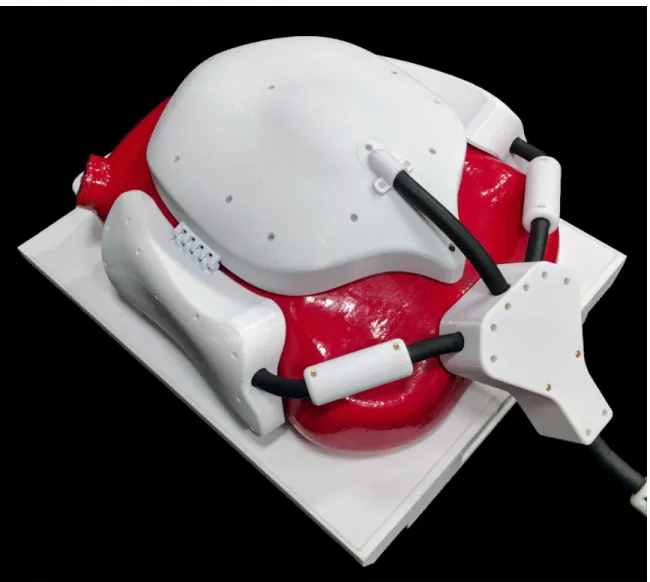
Individual loops were constructed from 16 gauge tin plated copper wire, with bridges bent into the wires to allow them to cross each other without touching. A schematic of the loop circuitry is shown in 4-1. Chapter 4 contains a detailed expla-nation of the function of the loop circuit.

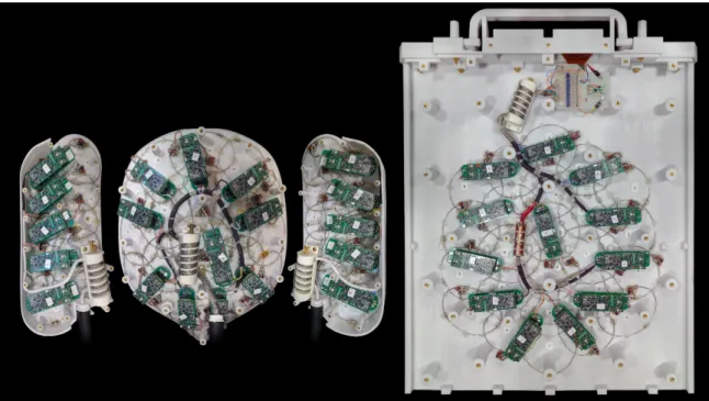
The finished coil is shown in figure 3-2 posed on the pregnant abdomen phantom used extensively in testing. A view of the internal construction and wiring is shown in figure 3-3.

3.3 Cable Traps

Precautions must be taken to prevent large common mode currents from developing on internal and external wiring during the RF transmit phase. Such uncontrolled currents could pose a fire/safety hazard, and at the very least would interfere with the sequence being run. Common mode chokes spaced every 20cm on all internal and external prevent the induced currents from growing too large. Due to the high magnetic field the array operates in, ferrite chokes are not an option. Instead, tuned resonant traps are constructed. Two types of traps were used in this array.

3.3.1 Helical Traps

The operation of the resonant helical traps visible in fig. 3-3 is easy to understand. The jacketed wire bundle is wound around a helical former to create an air core inductor. High voltage capacitors are then connected across the turns of the inductor, forming a parallel LC tank. At resonance, the trap presents a high impedance to common mode currents flowing in the jacket. This kind of trap can hold off hundreds of volts, and has a high Q. It is used as the first cable trap inside each array panel, and inside the foot end table plug.

Figure 3-3: View of internal array construction and wiring.

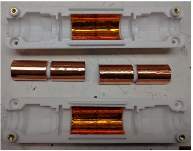
3.3.2 Bazooka Trap

The bazooka trap can be thought of as a physically short bazooka balun that has been electrically lengthened to 𝜆

4 by shunting the open end with a capacitor. A cylindrical

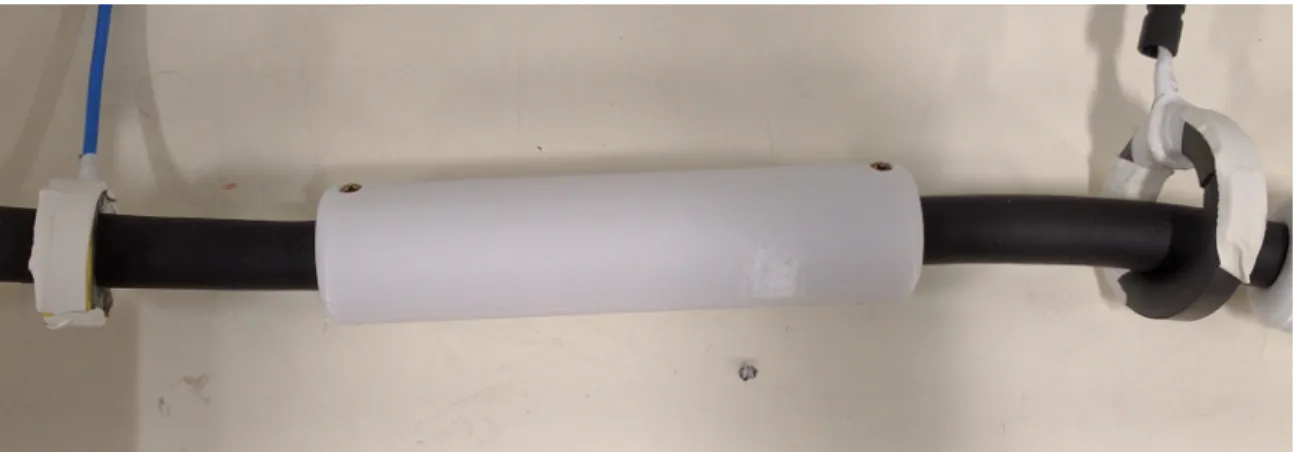
plastic spacer is printed in two halves. The outside surface of each half is covered in copper tape, with a gap left in the middle. The two halves are placed around the wire bundle and soldered together, and each end of the balun is soldered to the braided wire jacket. The gap in the copper tape is bridged with nonmagnetic capacitors selected such that the structure resonates at the desired frequency. An additional layer of copper shielding on the balun enclosure stabilizes the capacitance between the two ends of the balun so that external loading does not affect its resonant frequency. This kind of trap is more compact and consumes less wire length than the helical trap, but cannot hold off as much voltage and has a lower Q. It is placed periodically on long runs of external wiring.

Figure 3-4: Bazooka Balun before assembly.

Figure 3-6: Cable trap with current injection probes.

3.3.3 Trap Tuning

Both of the cable trap types described are narrow band, and must be properly tuned to function. This is accomplished through the use of a network analyzer and two current injection probes (fig. 3-6). Under the right measurement conditions, a prominent dip ( 20𝑑𝐵) in |𝑆12| around the resonance frequency can be observed.

Chapter 4

Loop Elements

The same basic loop circuit, shown in figure 4-1, is duplicated 64 times to create the full array. The components appearing inside the dashed green box exist on a small FR4 circuit board termed the "feed point board." Here, I will discuss the purpose and function of each part of this circuit. All capacitors used in the loop circuit are Voltronics Series 11 non-magnetic.

4.1 Active Detuning

The loop is a resonant circuit that is strongly coupled to the volume surrounding it. It is necessary to spoil this resonance during the high power RF transmit pulses so that excessive currents are not induced in the loop. Such unintended energy deposition could adversely affect transmit homogeneity, damage the array, or create a safety hazard. Selective detuning is achieved by switching an inductor across one of the loop capacitors, creating a parallel resonant tank that behaves as an open circuit in the loop at 𝜔𝐿.

A DC bias current of about 120𝑚𝐴 is injected on the line marked BIAS in figure 4-1. This bias current flows through a PIN diode 𝐷1 (MACOM MA47461F-1072),

creating an RF short and effectively switching 𝐿𝑇 𝑅𝐴𝑃 across 𝐶𝑆3. 𝐿𝑇 𝑅𝐴𝑃 is an

ad-justable air core inductor, and is hand tuned to resonate with 𝐶𝑆3 at precisely 𝜔𝐿.

preventing current from circulating in the loop. As soon as the bias current is removed and the diode recovers, the trap is disabled and the loop once again becomes tuned. The 𝑄 of this active detuning trap is kept high by using a relatively high value high Q inductor for 𝐿𝑇 𝑅𝐴𝑃. In this case, we used a 60𝑛𝐻 hand wound inductor made

with 16 AWG enameled copper wire.

The bias current is injected through a bias tee formed by 𝐿𝐵𝐼𝐴𝑆 (3.3𝑢𝐻 Coilcraft)

and a 1𝑛𝐹 capacitor to prevent leakage or injection of RF signal from/to the loop on the bias line.

4.2 Passive Detuning

The active detuning strategy is sufficient for assurance of image quality and protection from hardware damage, but a passive method is required to ensure patient safety in the event of an electrical failure. The crossed diode pair 𝐷2 (BAV99) clamps the

voltage across 𝐶𝑆3 and 𝐿𝑇 𝑅𝐴𝑃 to safe levels, passively enabling the trap if the energy

stored in the loop gets too high. Other designs might also include RF fuses in the loop circuit, but the loops employed in this array are all small enough that this was not necessary.

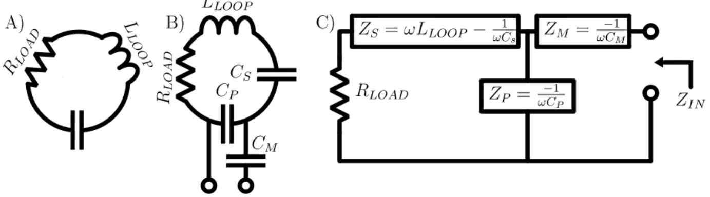
4.3 Loop Model

The essence of the wire loop receive elements used in this array is a damped series resonant circuit, shown in figure 4-2A. The loop has a distributed inductance by nature of its geometry, and is broken at regular intervals by discrete capacitors. Wire and component resistances and (more importantly) inductive coupling to adjacent conductive materials reduces the loop 𝑄 to a finite value. This effect is modeled by a series resistor with value 𝑅𝐿𝑂𝐴𝐷 =

√︁

𝐿 𝐶 ·

1 𝑄

BIAS 𝐷1 𝐷2 𝐶𝑃 𝐶𝑀 𝐶𝑆3 𝐶𝑆2 𝐶𝑆1 1nF 1nF 𝐿𝑇 𝑅 𝐴𝑃 𝐿𝐵 𝐼 𝐴𝑆 𝐿𝑃 𝑅 𝐸

𝐿𝐿𝑂𝑂𝑃 𝐶𝑆 𝐶𝑃 𝑅𝐿𝑂 𝐴𝐷 𝑅𝐿𝑂 𝐴 𝐷 𝐿 𝐿𝑂 𝑂 𝑃 𝐶𝑀 𝑅𝐿𝑂𝐴𝐷 C) A) _{𝑍𝑆 = 𝜔𝐿𝐿𝑂𝑂𝑃 −} 1 𝜔𝐶𝑠 𝑍𝑃 = _𝜔𝐶−1 𝑃 B) _{𝑍𝑀 =} −1 𝜔𝐶𝑀 𝑍𝐼𝑁

Figure 4-2: Loop circuit models.

4.4 Complete Loop Circuit

Figure 4-2B shows the creation of an output port in the loop circuit. The total loop capacitance is split into 𝐶𝑃, across which the output port is formed, and 𝐶𝑆. A series

capacitor 𝐶𝑀 is added to one terminal of the output port. In the first part of the

following analysis, grouping components values into the block impedances defined in eq. 4.1 and fig. 4-2C results in clearer and more compact expressions, so I have made that substitution. 𝑋𝑆(𝜔) = 𝜔𝐿𝐿𝑂𝑂𝑃 − 1 𝜔𝐶𝑆 𝑋𝑃(𝜔) = −1 𝜔𝐶𝑃 𝑋𝑀(𝜔) = −1 𝜔𝐶𝑀 (4.1)

4.5 Loop Circuit Analysis

The loop circuit has an input impedance of 𝑍𝐼𝑁 at its port, as defined in equation

4.2. This impedance can be split into its real and imaginary parts, 𝑅𝐼𝑁 and 𝑋𝐼𝑁,

shown in equations 4.3 and 4.4.

𝑍𝐼𝑁 = (𝑗𝑋𝑝(𝜔)) ‖ (𝑗𝑋𝑆(𝜔) + 𝑅𝐿𝑂𝐴𝐷) + 𝑗𝑋𝑀(𝜔)

= 𝑗𝑋𝑃(𝜔)(𝑗𝑋𝑆(𝜔) + 𝑅𝐿𝑂𝐴𝐷) 𝑗(𝑋𝑃(𝜔) + 𝑋𝑆(𝜔)) + 𝑅𝐿𝑂𝐴𝐷

+ 𝑗𝑋𝑀(𝜔)

𝑅𝐼𝑁 = 𝑅𝑒(𝑍𝐼𝑁) = 𝑋𝑃(𝜔) 2 𝑅𝐿𝑂𝐴𝐷 𝑅𝐿𝑂𝐴𝐷2+ (𝑋𝑃(𝜔) + 𝑋𝑆(𝜔))2 (4.3) 𝑋𝐼𝑁 = 𝐼𝑚(𝑍𝐼𝑁) = 𝑋𝑃(𝜔)(𝑅𝐿𝑂𝐴𝐷2+ 𝑋𝑆(𝜔)(𝑋𝑃(𝜔) + 𝑋𝑆(𝜔))) 𝑅𝐿𝑂𝐴𝐷2+ (𝑋𝑃(𝜔) + 𝑋𝑆(𝜔))2 + 𝑋𝑀(𝜔) (4.4)

4.6 Loop Component selection

4.6.1 Loop Circuit Considerations

Minimizing Preamp Noise Figure

The vendor supplied preamplifier is designed to achieve minimum noise figure when presented with a purely real 50Ω load at its input. Therefore, component values should be selected such that 𝑅𝐼𝑁 = 50Ω and 𝑋𝐼𝑁 = 0Ω. Call this optimal input

impedance 𝑍𝐼𝑁𝑂𝑃 𝑇.

Preamp Decoupling

Preamp decoupling is usually achieved by resonating a capacitor in the loop (𝐶𝑃 in

figure 4-2) with an inductor in series with one terminal of the output port (in the same position as 𝐶𝑀 in figure 4-2) through the input of the preamplifier. In our

case, however, the inductance is integrated into the preamplifier itself. I measure the inductance of the preamplifer input to be roughly 130𝑛𝐻 at 123.25𝑀𝐻𝑧. The details of the preamp topology are unavailable to me, so I simply consider it to have an impedance of 𝑍𝑃 𝑅𝐸 = 𝑗𝜔𝐿𝑃 𝑅𝐸, which is transformed to 𝑍𝑃 𝑅𝐸′ (as shown in

equation 4.5) by the short length of coaxial cable (with characteristic impedance 𝑍0)

connecting the preamp to the loop. 𝑍𝑃 𝑅𝐸′(𝜔) = 𝑍0·

𝑍𝑃 𝑅𝐸(𝜔) − 𝑗𝑍0· tan(2𝜋 ·𝐿𝐶𝑂𝐴𝑋_𝜆 )

𝑍0− 𝑗𝑍𝑃 𝑅𝐸(𝜔) · tan(2𝜋 ·𝐿𝐶𝑂𝐴𝑋_𝜆 )

𝑋𝑃 𝑅𝐸′(𝜔) = 𝐼𝑚(𝑍𝑃 𝑅𝐸′(𝜔)) (4.6)

In any case, preamp decoupling is achieved when 𝐶𝑃, 𝐶𝑀, and the transformed

preamp input impedance resonate together, as defined in equation 4.7.

𝑋𝑃(𝜔) + 𝑋𝑀(𝜔) + 𝑋𝑃 𝑅𝐸′(𝜔) = 0 (4.7)

4.6.2 Loop Resonance

I define loop resonance as occurring when 𝑋𝑃 + 𝑋𝑆 = 0, at a frequency of 𝜔0 (eq.

4.8). In this case, the equations for 𝑅𝐼𝑁 and 𝑋𝐼𝑁 simplify to equations 4.9 and

4.10 respectively. One can begin to see how components could be selected to set 𝑅𝐼𝑁

⃒ ⃒

𝜔=𝜔0 = 𝑅𝑒(𝑍𝐼𝑁𝑂𝑃 𝑇), but with the topology we’ve selected it is impossible to

achieve 𝑋𝐼𝑁

⃒ ⃒

𝜔=𝜔0 = 0. You could do both if you changed 𝐶𝑀 to an inductor, but

then it becomes impossible to meet the preamp decoupling condition (eq. 4.7). 𝜔0 = √︂ 𝐶𝑃 + 𝐶𝑆 𝐶𝑃𝐶𝑆𝐿𝐿𝑂𝑂𝑃 (4.8) 𝑅𝐼𝑁 ⃒ ⃒ 𝜔=𝜔0 = 𝐶𝑆𝐿𝐿𝑂𝑂𝑃 𝑅𝐿𝑂𝐴𝐷𝐶𝑃(𝐶𝑃 + 𝐶𝑆) (4.9) 𝑋𝐼𝑁 ⃒ ⃒ 𝜔=𝜔0 = − √︃ 𝐶𝑆𝐿𝐿𝑂𝑂𝑃 𝐶𝑃(𝐶𝑃 + 𝐶𝑆) · 𝐶𝑀 + 𝐶𝑃 𝐶𝑀 (4.10)

4.6.3 Off resonance behavior

It is not necessary that the loop be tuned to resonate precisely at the frequency of interest. The position of 𝜔0 relative to that of the Lamor frequency 𝜔𝐿 is another

Capacitive Divider Ratio

Consider choosing 𝐶𝑃 and 𝐶𝑆 to achieve loop resonance at a frequency a factor 𝛼

away from 𝜔𝐿, so that 𝜔0 = 𝛼 · 𝜔𝐿. We can quickly eliminate 𝐶𝑆 from eq. 4.8.

Whatever 𝐶𝑃, 𝛼, and 𝜔𝐿 we choose will imply eq. 4.11 for 𝐶𝑆.

𝐶𝑆(𝐶𝑃, 𝛼, 𝜔𝐿) =

𝐶𝑃

𝐶𝑃𝐿𝐿𝑂𝑂𝑃𝛼2𝜔𝐿2− 1

(4.11) Plugging eq. 4.11 into eq. 4.3, then solving 𝑅𝐼𝑁 = 𝑍𝐼𝑁𝑂𝑃 𝑇 for 𝐶𝑃, we get eq.

4.12. 𝐶𝑃(𝛼, 𝜔𝐿) = 1 𝜔𝐿 √︃ 𝑅𝐿𝑂𝐴𝐷 𝑍𝐼𝑁𝑂𝑃 𝑇(𝑅𝐿𝑂𝐴𝐷 2_{+ (𝛼}2_{− 1)}2_𝜔 𝐿2𝐿𝐿𝑂𝑂𝑃2) (4.12) Choosing 𝛼 and 𝐶𝑀

The only remaining free parameters are 𝛼 and 𝐶𝑀. They must be chosen to achieve

purely real input impedance (𝑋𝐼𝑁 = 0) and preamp decoupling (𝑋𝑃(𝜔𝐿) + 𝑋𝑀(𝜔𝐿) +

𝑋𝑃 𝑅𝐸′(𝜔𝐿) = 0). Plugging in 𝐶𝑆 and 𝐶𝑃 from above into these two requirements

results in a system of equations 4.13. Constraining 𝛼 to be positive, this system has single solution: 𝛼 as in eq. 4.14 and 𝐶𝑀 as in eq. 4.15.

⎧ ⎪ ⎨ ⎪ ⎩ −1 𝜔𝐿𝐶𝑀 + (𝛼2_−1)𝜔 𝐿𝐿𝐿𝑂𝑂𝑃𝑍_{𝐼𝑁𝑂𝑃 𝑇} 𝑅𝐿𝑂𝐴𝐷 − 1 𝜔𝐿𝐶𝑃(𝛼,𝜔𝐿) = 0 −1 𝜔𝐿𝐶𝑀 + 𝜔𝐿𝐿𝑃 𝑅𝐸− 1 𝜔𝐿𝐶𝑃(𝛼,𝜔𝐿) = 0 (4.13) 𝛼 = √︃ 1 + 𝐿𝑃 𝑅𝐸𝑅𝐿𝑂𝐴𝐷 𝐿𝐿𝑂𝑂𝑃𝑍𝐼𝑁𝑂𝑃 𝑇 (4.14)

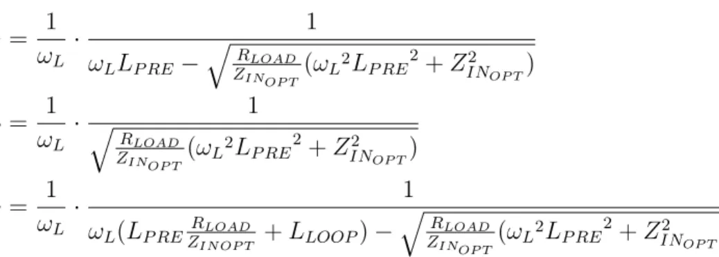
4.6.4 Optimal Component values

With 𝛼 uniquely determined, 𝐶𝑀, 𝐶𝑃, and 𝐶𝑆 are each fully constrained. Our final

𝐶𝑀 = 1 𝜔𝐿 · 1 𝜔𝐿𝐿𝑃 𝑅𝐸− √︁_𝑅 𝐿𝑂𝐴𝐷 𝑍_{𝐼𝑁𝑂𝑃 𝑇}(𝜔𝐿 2_𝐿 𝑃 𝑅𝐸2+ 𝑍_𝐼𝑁2 _{𝑂𝑃 𝑇}) 𝐶𝑃 = 1 𝜔𝐿 · _√︁ 1 𝑅𝐿𝑂𝐴𝐷 𝑍_{𝐼𝑁𝑂𝑃 𝑇}(𝜔𝐿 2_𝐿 𝑃 𝑅𝐸2+ 𝑍𝐼𝑁2 𝑂𝑃 𝑇) 𝐶𝑆 = 1 𝜔𝐿 · 1 𝜔𝐿(𝐿𝑃 𝑅𝐸_𝑍𝑅_{𝐼𝑁 𝑂𝑃 𝑇}𝐿𝑂𝐴𝐷 + 𝐿𝐿𝑂𝑂𝑃) − √︁_𝑅 𝐿𝑂𝐴𝐷 𝑍_{𝐼𝑁𝑂𝑃 𝑇}(𝜔𝐿2𝐿𝑃 𝑅𝐸 2_{+ 𝑍}2 𝐼𝑁𝑂𝑃 𝑇) (4.15)

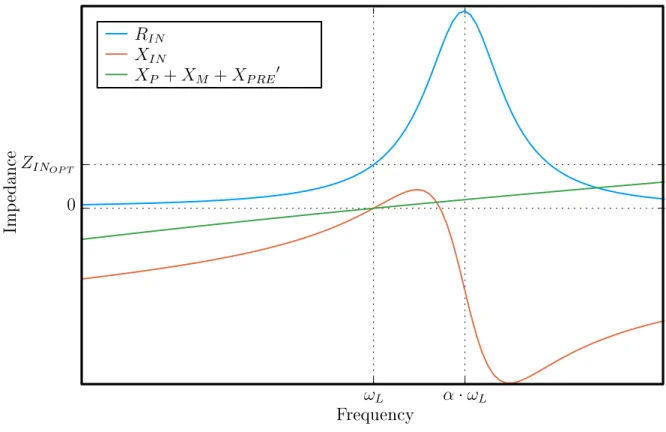
4.6.5 Verifying Optimal Component Values

Figure 4-3 illustrates the success of this component selection strategy in simulta-neously achieving optimal input impedance and preamp decoupling. The impedance plots shown are based on estimated parameters of a loop in the belly panel. Numerical values for this simulation are summarized in tables 4.1 and 4.2.

𝛼 · 𝜔𝐿 𝜔𝐿 Frequency 0 𝑍𝐼𝑁𝑂𝑃 𝑇 Imp edance 𝑅𝐼𝑁 𝑋𝐼𝑁 𝑋𝑃 + 𝑋𝑀 + 𝑋𝑃 𝑅𝐸′

Figure 4-3: Loop impedances vs. frequency with optimal component values.

Table 4.1: Loop simulation parameters Parameter Value 𝑅𝐿𝑂𝐴𝐷 10Ω 𝐿𝐿𝑂𝑂𝑃 247𝑛𝐻 𝐿𝑃 𝑅𝐸 130𝑛𝐻 𝑍𝐼𝑁𝑂𝑃 𝑇 50Ω 𝜔𝐿 123.25𝑀 𝐻𝑧

Table 4.2: Calculated optimal component values Parameter Value

𝐶𝑀 25.8𝑝𝐹

𝐶𝑃 25.8𝑝𝐹

𝐶𝑆 8.0𝑝𝐹

Chapter 5

Figures of Merit

The aim of this project was to create a custom coil that performs better than ex-isting arrays in a particular application. Our primary means of evaluating relative performance is direct comparison of two related performance metrics: SNR maps and SENSE geometry factor (g-factor) maps. A brief discussion of each follows. For a complete treatment, see the original SENSE paper: [6].

5.1 Signal to Noise Ratio Maps

In MRI, SNR is commonly defined as the ratio between signal amplitude and the standard deviation of noise. The MR signal to noise ratio provided by any coil or coil array varies as a function of space. A heatmap of SNR in absolute SNR units as defined by Kellman and McVeigh [3] in a given plane is a useful visual tool that can be used to judge whether a coil is well suited to imaging in a particular region of interest such as the fetal brain or placenta. An SNR map is easy to generate for a single coil. One can simply run an imaging sequence with intrinsically high SNR twice; once with an initial RF excitation and once without. The first sequence should produce an image that is dominated by the MR signal, and the second sequence produces a noise only image. A SNR map in conventionally defined SNR units is obtained by dividing the first image by the standard deviation of the noise only image.

on the method used to combine data from individual elements. The Roemer paper [8] describes an optimal way of combining array coil data in the spatial domain that results in maximum SNR and normalized noise intensity in every voxel of the resulting image. First, a complete image is acquired and reconstructed from every element in the array. Next, a sample of pure noise data is acquired to generate a channel noise covariance matrix Ψ, of which a single element Ψ𝑖𝑗 is the noise covariance between

receivers 𝑖 and 𝑗.

Now, the individual coil images are combined on a voxel by voxel basis. For a single voxel, arrange the values 𝑆𝑖 of that voxel in each of the individual coil images

in a vector 𝑆. Similarly, arrange the sensitivities of each coil to the voxel under consideration in a vector 𝐶. The matrix equation for the voxel intensity in the optimal SNR uniform noise image is then eq. 5.1. If the individual coil images have sufficiently high SNR, then 𝑆 serves as a good approximation of 𝐶, and equation 5.1 simplifies to 5.2. If it is assumed that there is no noise correlation between distinct channels and that all channels are identically loaded, Ψ becomes proportional to the identity matrix, and the optimal SNR formula simplifies to 5.3. This is equivalent to summing the squared magnitudes of the uncombined images, then taking the square root of the result.

𝐼𝑂𝑃 𝑇 = 𝐶𝐻Ψ−1𝑆 √ 𝐶𝐻_Ψ−1_𝐶 (5.1) 𝐼𝐶𝑂𝑉 = √ 𝑆𝐻_Ψ−1_𝑆 (5.2) 𝐼𝑅𝑆𝑂𝑆 = √ 𝑆𝐻_𝑆 (5.3) SNR Map Equations

As stated, the optimal combination method is constructed to create a uniform noise image, where every voxel in the final image has unity noise standard deviation. So, the expression for a voxel in an optimal combination method SNR map is the same

as the expression for a voxel in the image: 𝑆𝑁 𝑅𝐶𝑂𝑉 = 𝐼𝐶𝑂𝑉 =

√

𝑆𝐻_Ψ−1_𝑆 (5.4)

For the RSOS method, the SNR map is calculated as: 𝑆𝑁 𝑅𝑅𝑆𝑂𝑆 =

𝑆𝐻𝑆 √

𝑆𝐻_Ψ𝑆 (5.5)

5.2 SENSE Geometry Factor

5.2.1 K-space Sampling for the 2DFT

The basic Fourier abstraction used in traditional 2D MRI with Cartesian k-space sampling illuminates a fundamental constraint on imaging speed: k-space traversal speed.

Sampling Constraints

The spatial extents of an image dictate the spectral spacing of samples that must be acquired to encode it with the DFT [5]. In order to 2D Fourier encode an image of width 𝐹 𝑂𝑉𝑥 and height 𝐹 𝑂𝑉𝑦, k-space samples must be spaced _{𝐹 𝑂𝑉}1_𝑋 apart in the

𝑘𝑥 direction and _{𝐹 𝑂𝑉}1

𝑌 apart in the 𝑘𝑦, direction, as defined in eq. 5.6.

𝐹 𝑂𝑉𝑥 = 1 𝛿𝑘𝑥 𝐹 𝑂𝑉𝑦 = 1 𝛿𝑘𝑦 (5.6) The spatial resolution of an image dictates the extents of spectral data that must be acquired to encode it with the DFT. In order to 2D Fourier encode an image with voxels 𝛿𝑥 wide and 𝛿𝑦 tall, data must be sampled over a period of approximately _𝛿1_𝑥

𝛿𝑥 ≈ 1 2𝑘𝑥𝑚𝑎𝑥 𝛿𝑦 ≈ 1 2𝑘𝑦𝑚𝑎𝑥 (5.7) It is clear that the number k-space samples needed to resolve an image grows linearly with both FOV and voxel density, and that the maximum extents of those samples in k-space increases linearly with voxel density. K-space is sampled by travers-ing a continuous path that sequentially visits the coordinates of each sample. The maximum speed of k-space traversal is fundamentally limited by patient safety consid-erations and technological limitations. So, for a given maximum speed and optimum path, there is a minimum acquisition time for a fully sampled 2DFT sequence with a given FOV and spatial resolution.

Cartesian Undersampling

An imaging sequence can be accelerated by skipping some points in k-space, then attempting by some means to reconstruct a complete image from incomplete k-space data. In the case of cartesian sampling for the 2DFT, a natural strategy is to regularly skip entire lines of k-space data in one dimension [6], for example acquiring every other line (R=2) or every third line (R=3). The effect of this regular undersampling strategy is to effectively increase 𝛿 by a factor of R, and to accordingly decrease 𝐹 𝑂𝑉 by the same factor of R. This causes parts of the object being imaged that lie outside of the reduced FOV to wrap around the edges of that FOV and alias onto other voxel positions.

SENSE

The Pruessmann paper [6] introduced the strategy of "Sensitivity Encoding" as a means of undoing the aliasing induced by undersampling. In an array coil, different receive elements have different spatial sensitivity profiles. These varying sensitivities provide different "views" of the same aliased image, and this extra information is used to unfold the aliased image on a pixel by pixel basis.

Consider an array with 𝑛𝐶 individual elements, each with a unique view of a voxel

location that, in the reduced FOV image, represents a superposition of 𝑛𝑃 physical

voxel locations. A sensitivity matrix 𝑆 is constructed to describe the sensitivity of each receive element to each of the voxel positions that are aliased into a single pixel in the final image. An individual element 𝑆𝛾,𝜌 in this matrix represents the sensitivity

of receive element number 𝛾 to superimposed pixel number 𝜌. The values of the voxel in the reduced FOV images from each receive element are arranged in a vector ⃗𝑎 of length 𝑛𝐶. Similar to in the previous section, a 𝑛𝐶 × 𝑛𝐶 receiver noise covariance

matrix Ψ is constructed from a noise-only acquisition. The unfolding matrix is then:

𝑈 = (𝑆𝐻Ψ−1𝑆)−1𝑆𝐻Ψ−1 (5.8)

The vector of image values in the 𝑛𝑝 voxels of the unaliased image are estimated

by:

⃗𝑣 = 𝑈⃗𝑎 (5.9)

This unfolding process is repeated for every voxel in the reduced FOV image.

SENSE g-factor

By accelerating an image acquisition by a factor of 𝑅, we expect that the SNR of the resulting image must correspondingly decrease by a factor of _√1

𝑅 [5]. Usually,

though, imperfect conditioning of the sensitivity matrix results in a a steeper SNR penalty. The extent to which SENSE underperforms the best case SNR penalty is characterized by the geometry factor, or g-factor, defined in eq. 5.10. The g-factor varies as a function of space, and is defined for each voxel in the full FOV image. It is called the geometry factor because it depends largely on the geometry of the receive array. When more independent views of an aliased pixel are available, a higher acceleration factor can be attempted without poor conditioning amplifying noise to an unacceptable degree. This is the mission of the array coil.

𝑔𝑆𝐸𝑁 𝑆𝐸 = 1 √ 𝑅 · 𝑆𝑁 𝑅𝐹 𝑈 𝐿𝐿 𝑆𝑁 𝑅𝐴𝐶𝐶𝐸𝐿 (5.10) Plots of 2D SENSE g-factor maps in a given slice are a useful graphical tool for assessing the ability of an array to support a given acceleration factor along a particular dimension (or, along two dimensions simultaneously.) SENSE g-factor is widely used to compare the acceleration capability of different coil arrays because it is straightforward to compute and gives insights into the fundamental ability of an array to enable acceleration using any method. Still, it is important to note that unique formulations of g-factor have been developed for other acceleration methods, such as SMASH and GRAPPA [1].

Chapter 6

Methods

6.1 Bench Tests

6.1.1 Intercoil Coupling and Reflection Coefficient

Measure-ments

A network analyzer connected directly to loop output ports was used to measure coupling between neighboring coil elements (𝑆12), and to measure individual coil

output reflection coefficients (𝑆11). For each of theses tests, the output power of the network analyzer was reduced to -25dBm and the coil was appropriately loaded by a test phantom. This test configuration was used during the iterative geometric decoupling adjustment process, where the loops are manually bent and reconfigured to minimize neighbor-to-neighbor coupling.

6.1.2 Loop Detuning and Preamp Decoupling Verification

The active detune capability and preamp decoupling performance were tuned and characterized using a pair of decoupled (𝑆12< 70𝑑𝐵) inductive probes loosely coupled

to the loop under test. In this arrangement, the 𝑆12 measurement between the two

probes is directly proportional to the current flowing in the loop [7]. Both the active detune capability and preamplifier decoupling strategy work by introducing a second

resonance near the loop resonance frequency, which "splits" the loop resonance into two peaks above and below the initial resonance frequency. The null between these peaks is moved to 𝜔𝐿 by adjustment of a tunable component. For the active detune

strategy, this tunable component is an adjustable air-core inductor (𝐿𝑇 𝑅𝐴𝑃 in fig.

4-1). For preamp decoupling, it is a trim capacitor (𝐶𝑀 in fig. 4-1).

6.2 MRI Data Acquisition and Reconstruction

Images of the pregnant abdominal phantom were acquired using both the 64 channel fetal coil and the standard combination of 16 channels from a 32 channel spine ar-ray and all channels from an 18 channel flexible body arar-ray. Three orthogonal slices (transverse, coronal, and sagital) intersecting the fetal brain compartment were care-fully duplicated using both array configurations. An extremely high SNR PD weighted 2DGRE sequence (𝑇 𝑅 = 3500𝑚𝑠, 𝑇 𝐸 = 4𝑚𝑠, 𝐹 𝐴 = 45∘_{, 𝐹 𝑂𝑉 = 400𝑚𝑚, 𝛿 ≈}

2𝑚𝑚 × 2𝑚𝑚 × 7𝑚𝑚, 𝐵𝑊 = 180𝐻𝑧/𝑝𝑥) was chosen so that each of the uncom-bined coil images has decent SNR (> 20) in the deep central region of the fetal brain compartment, and thus can be taken as an accurate approximation of a coil sensitivity map [8]. The same sequence was run with the reference TX voltage set to 0𝑉 to acquire noise-only data for the generation of a noise covariance matrix Ψ. Data were acquired on a 3T Magnetom Skyra System (Siemens Healthcare, Erlangen, Germany).

Covariance weighted SNR maps and SENSE g-factor maps were computed offline using the resulting raw data. For the fetal coil, single channel SNR maps were gen-erated by dividing each of the 64 uncombined coil images by the standard deviation of a corresponding noise only image. The mean value of each single channel SNR map was computed inside an ROI (𝐴 = 29 voxels) in the fetal brain region of the anthropomorphic phantom as a means of assessing the relative importance of each component in the array geometry.

Chapter 7

Results

7.1 Covariance Weighted SNR Maps

Covariance weighted SNR maps for three perpendicular slices chosen to intersect the fetal brain compartment are shown in figs. 7-1, 7-2, and 7-3. In each cross section, it can be seen that the fetal array provides greatly increased SNR in the periphery of the phantom, but only narrowly outperforms the standard array configuration in the deep central region where the fetus is actually located. In this particular dataset, SNR was improved by approximately 5% inside the fetal brain compartment in each of the three slices.

Figure 7-1: Comparative covariance weighted SNR maps, transverse slice through fetal phantom brain.

Figure 7-2: Comparative covariance weighted SNR maps, coronal slice through fetal phantom brain.

Figure 7-3: Comparative covariance weighted SNR maps, sagital slice through fetal phantom brain.

7.2 Inverse G-Factor Maps

As compared to the standard combination of the 32 channel spine array and 18 channel flexible body array, the 64 channel fetal coil allows increase in SENSE acceleration factor from four to five in the right-left direction (figs. 7-4, 7-6) and 3 to 4 in the head-foot direction (figs. 7-7, 7-8) while maintaining acceptably low noise amplification levels. Both array configurations have poor acceleration capability in the anterior-posterior direction (figs. 7-5, 7-9). Note that in order to increase contrast in the relevant range, the color scale on these maps goes from 0.5 to 1, not 0 to 1.

Figure 7-10 shows inverse SENSE g-factor maps for 2D acceleration in the head-foot and left-right directions, comparing array performance at 𝑅 = (3, 4) and 𝑅 = (4, 5). This comparison was chosen to highlight the best case improvement in accel-eration capability provide by the fetal coil. Inside a large central ROI covering the entire fetus, the fetal coil maintains 𝑔 ≤ 1.5 with 𝑅 = 4, 5 while the product array

Figure 7-4: Comparative inverse SENSE g-factor maps, transverse slice through fetal phantom brain, acceleration in right-left direction.

Figure 7-5: Comparative inverse SENSE g-factor maps, transverse slice through fetal phantom brain, acceleration in anterior-posterior direction.

only achieves 𝑔 ≤ 3.9. In the same ROI, they have mean inverse g-factors (1/𝑔) of 0.82 and 0.43, respectively. Roughly speaking, the fetal coil has noise amplification levels at 𝑅 = (4, 5) that are comparable to the standard array configuration at 𝑅 = (3, 4). This represents a 67% increase in overall acceleration factor.

7.3 Noise Matrices

Figure 7-11 shows the absolute value of a noise covariance matrix Ψ calculated from this dataset. Figure 7-12 shows the same data normalized along the diagonal so that the element with indices 𝑗, 𝑘 is the correlation coefficient for channels 𝑗 and 𝑘. The correlation coefficient is equal to 1 when 𝑗 = 𝑘.

Figure 7-6: Comparative inverse SENSE g-factor maps, Coronal slice through fetal phantom brain, acceleration in right-left direction.

Figure 7-7: Comparative inverse SENSE g-factor maps, coronal slice through fetal phantom brain, acceleration in head-feet direction.

Figure 7-8: Comparative inverse SENSE g-factor maps, sagital slice through fetal phantom brain, acceleration in head-feet direction.

Figure 7-9: Comparative inverse SENSE g-factor maps, sagital slice through fetal phantom brain, acceleration in anterior-posterior direction.

Figure 7-10: Comparative inverse SENSE g-factor maps, coronal slice through fetal phantom brain, acceleration in head-feet, right-left directions.

Figure 7-11: Absolute value of noise covariance matrix (|Ψ|).

Looking at the correlation coefficient matrix, several clearly defined regions of moderate correlation are apparent, with almost no correlation between different re-gions. The groupings follow the separation of elements into different array panels. From top left to bottom right, we see channels from the right side wing, left side wing, abdomen panel, and back panel.

7.4 Per-Element SNR

Figure 7-13 is a 1:4 scale diagram of the actual loop geometry used in the fetal array. Displayed inside each loop is the mean SNR of that channel inside the fetal brain ROI. It can be seen that elements in the back panel contributed most to overall SNR in the fetal brain compartment, followed by the belly panel and side wings.

Figure 7-12: Absolute value of inter-channel noise correlation coefficients (|√︀𝑑𝑖𝑎𝑔(Ψ)−1· Ψ ·√︀𝑑𝑖𝑎𝑔(Ψ)|).

Figure 7-13: Mean Single Element SNR values Inside the Fetal Phantom Brain (Top:Abdomen Panel and Side Wings, Bottom: Back panel)

Chapter 8

Discussion

The modest SNR improvement seen in unaccelerated imaging is likely attributed to the deep (nearly central) location of the fetal head where coil arrays with more than 16 elements already approach the ultimate SNR available [9]. Nonetheless, because the SNR is achieved with array elements with higher spatial frequency content sensitivity profiles, there is an improvement in acceleration capability.

The anterior and posterior array panels contribute overwhelmingly to the overall SNR in the fetal brain. Acceleration capability in the anterior-posterior direction was not substantially improved beyond what would be expected with just the two views of the phantom provided by anterior and posterior panels. The side wings do, however, benefit acceleration in the right-left direction.

Due to delays in IRB approval and subject recruitment, the array has thus far only been tested on the purpose built pregnant abdomen phantom. The phantom and array were designed based on the same segmented models of a pregnant volunteer, and so by design the coil fits the phantom very well. Since this close fit is one of the noted advantages of the 22 week fetal coil, further testing on a varied population of pregnant volunteers is needed to fully assess any performance improvement. Furthermore, practical considerations like patient comfort have not yet been evaluated.

Bibliography

[1] Felix A. Breuer, Stephan A R Kannengiesser, Martin Blaimer, Nicole Seiberlich, Peter M. Jakob, and Mark A. Griswold. General formulation for quantitative G-factor calculation in GRAPPA reconstructions. Magnetic Resonance in Medicine, 62(3):739–746, 2009.

[2] D. I. Hoult and Paul C. Lauterbur. The sensitivity of the zeugmatographic experi-ment involving human samples. Journal of Magnetic Resonance (1969), 34(2):425– 433, 1979.

[3] Peter Kellman and Elliot R. McVeigh. Image reconstruction in SNR units: A gen-eral method for SNR measurement. Magnetic Resonance in Medicine, 54(6):1439– 1447, 2005.

[4] T.H. Lee. The Design of CMOS Radio-Frequency Integrated Circuits. Cambridge University Press, 2004.

[5] Dwight G. Nishimura. Principles of magnetic resonance imaging. 1.1 edition, 2010.

[6] Klaas P Pruessmann, Markus Weiger, Markus B Scheidegger, and Peter Boesiger. SENSE: Sensitivity encoding for fast MRI. Magnetic Resonance in Medicine, 42(5):952–962, 1999.

[7] Arne Reykowski, Steven M. Wright, and Jay R. Porter. Design of Matching Net-works for Low Noise Preamplifiers. Magnetic Resonance in Medicine, 33(6):848– 852, 1995.

[8] P. B. Roemer, W. A. Edelstein, C. E. Hayes, S. P. Souza, and O. M. Mueller. The nmr phased array. Magnetic Resonance in Medicine, 16(2):192–225, 1990.

[9] Florian Wiesinger, Peter Boesiger, and Klaas P. Pruessmann. Electrodynamics and ultimate SNR in parallel MR imaging. Magnetic Resonance in Medicine, 52(2):376–390, 2004.