Aerodynamic response of turbomachinery blade rows to convecting density wakes

Aerodynamic Response of Turbomachinery Blade

Rows to Convecting Density Wakes

by

Hettithanthrige Sanith Wijesinghe

MEng. Aeronautical Engineering, Imperial College of Science, Technology and Medicine

(1996)

Submitted to the Department of Aeronautics and Astronautics in partial fulfillment of the requirements for the

degree of

Master of Science

Author-Certified by

Massachusetts Institute of Technology

September 1998

@

Detartfnent of Aeronautics and Astronautics

August 14th, 1998

Professor Eugene E. Covert

Professor of Aeronautics and Astronautics, Emeritus

A /Thesis Supervisor

Certified bvy

Dr. Choon S. Tan

I rincipal IFWseagcA Engineer, Dept. of Aeronautics and Astronautics

Accepted

by-MASSACHUSETS INSTITUTE

OF TECHNOLOGY

SEP 2

₁₉₉₈

I

IIQDOAar-Professor Jaime Peraire

Associate Professor of Aeronautics and Astronautics

Chairman, Department Graduate Committee

Aerodynamic Response of Turbomachinery Blade

Rows to Convecting Density Wakes

by

Hettithanthrige Sanith Wijesinghe

Submitted to the Department of Aeronautics and Astronautics on August 14th, 1998 in partial fulfillment of the requirements for the degree of

Master of Science

Abstract

Density wakes have been recently identified as a possible new source for high cycle fatigue failure in the compressor blades of modern turbomachinery. In order to charac-terize the density wake induced force and moment fluctuations in compressor blades a two-dimensional computational study has been conducted in viscous compressible flows with Mach numbers ranging from M, = 0.15 to Mo = 0.87 and flow Reynolds number Re(c, Uo) 700, 000.

Parametric tests were conducted at each flow Mach number to establish trends for the change in the maximum fluctuation of the blade force and moment coefficients with the changes in the density wake width 0.1 < w/c < 1.0 and the density ratio 0.25 < P2/P1 5 2.0. Results indicate the magnitude of the blade force and moment fluctuations to scale with (1) the non-dimensional density wake width w/c, (2) a non-dimensional density parameter

p* and (3) flow Mach number M,.

The viscous flow simulations have also indicated (1) periodic vortex shedding at the blade trailing edge and (2) separation bubbles on the blade suction surface which generate additional force and moment fluctuations with amplitudes +(10 - 100%) about the time averaged mean values. These flow features represent possible additional sources for high

cycle fatigue failure.

Simple functional relationships have also been derived at each flow Mach number to quantify the force and moment fluctuations described above. In addition a simple cascade flow model has been developed in conjunction with the computational study to help deter-mine the trends in the force and moment fluctuations with varying density wake properties and compressor geometries.

Thesis Supervisor: Prof. Eugene E. Covert

Title: Professor of Aeronautics and Astronautics, Emeritus

Thesis Supervisor: Dr. Choon S. Tan

ACKNOWLEDGMENTS

I would like to take this opportunity to acknowledge the love and support of my parents throughout the years. They have always allowed me to make my own decisions in life and have supported me through those decisions. I dedicate this thesis to them for helping me achieve all my goals.

I wish to thank Prof. Covert for providing me the opportunity to work on this project. His confidence and patience in me throughout these past 2 years is greatly appreciated. The analysis presented here is due in whole to the many discussion we have had. His excellent advising and mentoring throughout the project has made this a most pleasurable experience.

I would like to thank Choon for his thoughtful advice and comments and for helping me focus on the important research issues. I would also like to thank him for carefully proof reading this document many many times over. His suggestions have greatly improved the final version.

I would like to thank Prof. Frank Marble for his helpful discussions and comments. His original work provided the motivation for this research. I am also grateful to Becky Ramer for her initial work on this project.

A big thank you to Brian, Ken, Asif and Yang for their contribution to a lively office atmosphere and for always being available to discuss wild and crazy ideas! Thanks also to everyone at the GSC and the SLSA who successfully managed to divert my attention away from research and made sure I invested all my free time to help organize random events. It

has been a most worthwhile experience!

This work has been supported by the Air Force Office of Scientific Research and su-pervised by Major Brian Sanders, Program Manager, under contract number F49620-94-1-0202. This support is gratefully acknowledged.

CONTENTS

1.2 Physical Origin of Unsteadiness ...

1.3 Theoretical Background: Marble's Linearized Analysis 1.4 Inviscid Flow Simulations ...

1.4.1 Conclusions Based on Inviscid Results . . . . . 1.5 Questions Posed by the Current Research . . . .

1.6 Technical Approach ... ....

1.7 Thesis Contributions ... 1.8 Thesis Organization ...

2 Viscous Flow Solver

2.1 Features of The Viscous Flow Solver 2.2 Computational Grid ...

2.3 Cascade Geometry and Blade Profile 2.4 Density Wake Profile ...

2.5 Converged Solutions ... 27 . . . . .. . 27 . . . . 29 . . . . . 30 . . . . 33 . . . . . 37 . . . . . . . 37 . . . . .. . 38 . . . . . 40 . . . . . . . 41 43 . . . . . 43 . . . . 4 5 . . . . . . . . . . . . . . . 47 . . . . . . . . .. . 47 . . . . 49

2.6 Non-Dimensionalization ... ... ... 50

2.7 Summary ... ... 52

3 Viscous Results: Baseline Solutions 53 3.1 Baseline Force and Moment Response ... .. 53

3.1.1 Run 1: M. = 0.15 ... ... ... 54

3.1.2 Run 2: M , = 0.53 ... . ... .. 55

3.1.3 Run 3: M - 0.63 ... . ... .. 58

3.1.4 Run 4: M, = 0.87 ... 60

3.2 Vortex Shedding Frequency and Strouhal Number . ... 68

3.3 Summary ... . .... ... ... 70

4 Viscous Results: Response to Density Wakes 73 4.1 Force and Moment Profiles: Initial characterization . ... 74

4.2 Primary Response ... ... 76

4.2.1 General Flow Features ... .... . ... . 76

4.2.2 Run 4 : M , = 0.87 ... ... ... 79

4.2.3 Parametric Study ... ... ... . 84

4.3 Secondary Response ... .. ... . ... 93

4.3.1 General Flow Features ... ... 93

4.3.2 Parametric Study ... ... 96

4.3.3 Summary ... ... 101

5 Cascade Flow Model 107 5.1 Introduction ... .. ... ... 107

5.2 Modeling Assumptions ... ... ... ... 108

5.3 Induced velocities ... 110

5.3.1 Circulation Strength of The Counterrotating Vortices . ... 111

5.4 Solution Procedure ... . ... 113

5.5 Steady State Model Validation ... ... 115

5.6 Quasi-Steady Model Validation ... ... 118

5.7 Parametric Results ... ... ... ... 121

5.7.2 Lift and Moment Sensitivity to Cascade Geometry . ... 121

5.8 Summary ... .. . .. .... ... . 122

6 Conclusions And Further Work 125 6.1 Sum m ary . . . 125

6.2 Conclusions Based On The Viscous Results . ... 126

6.3 Conclusion Based On The Cascade Model Results . ... 126

6.4 Suggestions For Further Work ... ... 127

Bibliography 129

A Baseline Flow Results 133

B Viscous Flow Force And Moment Fluctuation Profiles 141

C Compressibility Scaling Of The Maximum Force and Moment

Fluctua-tions 169

LIST OF FIGURES

1-1 Density wake convecting through a compressor blade row. . ... 29

1-2 Lift coefficient fluctuation during passage of a density discontinuity over a flat plate. A is the position of the density discontinuity as it convects along the flat plate. The flat plate lies between I I < 1. . ... . 31

1-3 Moment coefficient fluctuation during passage of a density discontinuity over a flat plate. A is the position of density discontinuity as it convects along the flat plate. The flat plate lies between IAI < 1. . ... . . 32

1-4 Perturbation velocity vectors during passage of a density wake of width 0.2c and density ratio 0.5 through the NACA4F blade row. The flow is inviscid and incompressible. - = 0.65. ... ... 34

1-5 Fluctuation in (a) azimuthal force coefficient and (b) moment coefficient (positive counter-clockwise about the mid-chord) during passage of den-sity wakes. ACy = Cymax - Cymean, ACm = Cmmax - Cmmean where Cymean = 0.75, Cmmean = -0.13. Reproduced from Ramer. . ... 35

1-6 Maximum fluctuation in the azimuthal force coefficient (from steady state) during passage of density wakes through the NACA4F blade row. ACy = (Cymax - Cymean)/Cymean. Reproduced from Ramer. . ... 36

1-7 Maximum fluctuation in moment coefficient (from steady state) during pas-sage of density wakes through the NACA4F blade row. ACy = (Cymax -Cymean)/Cymean. Reproduced from Ramer. . ... 36

2-1 Schematic of the computational domain and boundary conditions. ... 45

2-2 O-grid detail at the blade leading edge. . ... . 46

2-4 50% span section of the LSRC Stator-B blade used for the viscous simula-tions. X denotes the location about which moments are evaluated (0.42c,

0.29c) ... . . .. ... 48

2-5 Density wake profile. w/c = 0.2, P2/P1 = 0.5. . . . . . 49 2-6 Convergence history for the L2 norm of density p x energy e. M" = 0.53.. 50

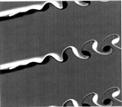
3-1 Vorticity contours indicating vortex shedding behind the blade trailing edge. M, = 0.15. Re(c, U,) = 620,000. The blade trailing edge is located at

0.40x (spacing of same-sign vortices) to the right of the left boundary. 56 3-2 Trajectory of consecutive shear layer wave peaks at an arbitrary time

in-stance. M, = 0.15 ... ... 56

3-3 Discrete fourier transform of the baseline force and moment coefficients. dft(X) is the discrete fourier transform of the time signal X. P =

non-dimensional frequency. M, = 0.15. . ... .... 57

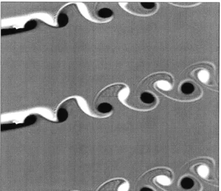
3-4 Vorticity contours indicating vortex shedding behind the blade trailing edge. M, = 0.53. Re(c, U,) = 630,000. The blade trailing edge is located at

0.35 x (spacing of same-sign vortices) to the right of the left boundary. 58

3-5 Trajectory of consecutive same-sign vortices at an arbitrary time instance. Mo = 0.53 ... ... 59 3-6 Discrete fourier transform of the baseline force and moment coefficients.

dft(X) is the discrete fourier transform of the time signal X. p =

non-dimensional frequency. Mc = 0.53. . ... .... 59

3-7 Vorticity contours indicating vortex shedding behind the blade trailing edge. M, = 0.63. Re(c, U.) = 580,000. The blade trailing edge is located at

0.50x (spacing of same-sign vortices) to the right of the left boundary. 60

3-8 Trajectory of consecutive same-sign vortices at an arbitrary time instance. Mo = 0.63 ... .. .. .. ... 61 3-9 Discrete fourier transform of the baseline force and moment coefficients.

dft(X) is the discrete fourier transform of the time signal X. p =

non-dimensional frequency. MO = 0.63. . ... .... 61

3-10 Mach number contours indicating extent of supersonic region in Run 4. Con-tours range from M = 1.0 to M = 1.5 in steps of 0.05. MO = 0.87. ... 62

3-11 Vorticity contour images indicating vortex shedding behind the blade trailing edge. M, = 0.87. Re(c, U,) = 800, 000. The blade trailing edge is located at 0.50x (spacing of same-sign vortices) to the right of the left boundary. 63

3-12 Trajectory of consecutive same sign vortices at an arbitrary time instance.

M, = 0.87 ... ... 63

3-13 Discrete fourier transform of the baseline force and moment coefficients. dft(X) is the discrete fourier transform of the time signal X. P =

non-dimensional frequency. M, = 0.87. . ... .... 64

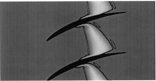
3-14 Pressure contours of the baseline solution for Run 4. The pressure waves can be seen as dark lines extending across the blade passage. M, = 0.87.

Re(c,U, ) = 0.8 x 106 ... . ... 65

3-15 Schlieren image of upstream traveling pressure waves behind a flat plate cascade from Lawaczeck. The Flow is from left to right. M(trailing edge)

0.80. Re(c,U,) = 0.8 x 106. ... ... ... 65

3-16 Location of upstream traveling pressure waves at specific time instances. T = 0.0 is an arbitrary time instance. M, = 0.87. . ... 66

3-17 Fluctuation in the shock wave position xs and the corresponding frequency spectrum. Mean shock location = 0.25x max(surf.distance). dft(X) is the discrete fourier transform of time signal X. . ... 67

3-18 Fluctuation in the static pressure rise across the shock wave ACps caused by the upstream traveling pressure waves. Mean ACps = 0.54. dft(X) is the discrete fourier transform of the time signal X. . ... 68

4-1 Fluctuations in (1) azimuthal force coefficient, (2) axial force coefficient and (3) moment coefficient (positive clockwise about the mid chord) during pas-sage of a density wake of width 0.2c and density ratio p2/Pl = 0.5. 3 distinct regions can be identified in the response. M. = 0.15. . ... . 75

4-2 Density contour image showing passage of density wake of width 0.2c and density ratio 0.5. Mo = 0.15. T = 0.04. . ... . 77

4-3 Density contour image showing passage of density wake of width 0.2c and density ratio 0.5. M, = 0.15. T = 0.53. . ... . . 77

4-4 Density contour image showing passage of density wake of width 0.2c and density ratio 0.5. M, = 0.15. T = 0.78. . ... . 78

4-5 Density contour image showing passage of density wake of width 0.2c and density ratio 0.5. M, = 0.15. T = 1.28. . ... . 78 4-6 Suction surface pressure distribution during passage of a density wake width

0.2c and density ratio 0.5. M, = 0.15. . ... .. 80 4-7 Change in blade pressure coefficient during passage of a density wake width

0.2c and density ratio 0.5. 7 = 0.32, M, = 0.15. . ... . 80 4-8 The change in (1) static pressure difference across the shock wave, (2)

az-imuthal force coefficient and (3) blade shock location during passage of a density wake width 0.1c and density ratio 0.25. M. = 0.87. . ... 83 4-9 Blade suction surface pressure contours showing the temporary suppression

of the blade passage shock wave during passage of a density wake of width 0.4c and density ratio 0.25. The dark band at x/c = 0.25 is the shock front.

M, = 0.87. ... ... ... 83

4-10 Changes in the maximum deflection of the shock wave as a function of the density wake width w/c and density parameter p*. . ... . 84 4-11 Maximum fluctuation in the force and moment coefficients as functions of

density wake width and density parameter p*. The straight lines joining data points are to help aid clarity. Mo = 0.15. . ... . 87 4-12 Maximum fluctuation in the force and moment coefficients as functions of

density wake width and density parameter p*. The straight lines joining data points are to help aid clarity. MO = 0.53. . ... . 87 4-13 Maximum fluctuation in the force and moment coefficients as functions of

density wake width and density parameter p*. The straight lines joining data points are to help aid clarity. M, = 0.63. . ... . 88 4-14 Maximum fluctuation in the force and moment coefficients as functions of

density wake width and density parameter p*. The straight lines joining data points are to help aid clarity. M, = 0.87. . ... . 88 4-15 Mach number contour image showing boundary layer deformation during

passage of a density wake of width 0.2c and density ratio 0.5. M. = 0.15.

4-16 Mach number contour image showing boundary layer deformation during passage of a density wake of width 0.2c and density ratio 0.5. M, = 0.15.

S= 1.03.. . . . . .... . . . . . . .. 94

4-17 Mach number contour image showing boundary layer deformation during passage of a density wake of width 0.2c and density ratio 0.5. Mo = 0.15.

7 = 1.28 ... ... ... ... 95

4-18 Mach number contour image showing boundary layer deformation during passage of a density wake of width 0.2c and density ratio 0.5. M" = 0.15. r = 1.53 .. . . . . . . . .. . 95 4-19 The fluctuation of the flow separation and re-attachment points of the suction

surface boundary layer during passage of a density wake of width 0.2c and density ratio 0.5. M , = 0.15 ... . ... 97 4-20 Vorticity contour image showing the disruption of regular vortex shedding

behind the blade trailing edge. The density wake is located 1.0c downstream of the trailing edge entrained inside the vortex wake. T = 3.1, w/c = 0.2,

P2/P1 = 0.5, M , = 0.87 ... ... 97

4-21 Discrete fourier transform of the secondary response force and moment coeffi-cient fluctuations. w/c = 0.2, P2/P1 = 0.5, M, = 0.87. dft(X) is the discrete fourier transform of the time signal X. Cp = non-dimensional frequency. . . 98 4-22 The maximum change in the suction surface separation point from the mean

baseline position as a function of wake width and density ratio. M, = 0.15 99 4-23 The maximum change in the suction surface separation point from the mean

baseline position as a function of wake width and density ratio. M" = 0.53. 100 4-24 The maximum change in the suction surface separation point from the mean

baseline position as a function of wake width and density ratio. M, = 0.63. 101 4-25 The maximum change in the suction surface separation point from the mean

baseline position as a function of wake width and density ratio. M, = 0.87. 102 4-26 The maximum fluctuation in the blade azimuthal force, axial force and

mo-ment coefficients in the secondary response region for varying density wake widths and density ratios. Moo = 0.15. . ... . . . 102

4-27 The maximum fluctuation in the blade azimuthal force, axial force and mo-ment coefficients in the secondary response region for varying density wake widths and density ratios. M, = 0.53 ... ... .. . . .. . . 103

4-28 The maximum fluctuation in the blade azimuthal force, axial force and mo-ment coefficients in the secondary response region for varying density wake widths and density ratios. M, = 0.63. . ... .. 103

4-29 The maximum fluctuation in the blade azimuthal force, axial force and mo-ment coefficients in the secondary response region for varying density wake widths and density ratios. M, = 0.87. . ... .. 104

5-1 Model schematic indicating flat plate cascade and counterrotating vortex pairs. 109

5-2 Change in circulation strength of the convecting vortices. v= sjl + s2 where ( is the location of the convecting vortex and sl and S2 are constants which ensure the tanh function is evaluated between -3 and +3. . ... 112

5-3 Cascade model results for the change in cascade interference coefficient Clcascade/Clairfoil with space-chord ratio and stagger angle. No. of panels = 1. . ... 115

5-4 Weinig's conformal mapping prediction for the cascade interference coefficient ko (Clcascade /Clairfoil) as a function of stagger angle -yeff and space-chord ratio (s/C)eff. .... ... .. . ... 116 5-5 Cascade model results for the change in cascade interference coefficient Clcascade/Clairfoil

with space-chord ratio and stagger angle. No. of panels = 5. . ... 117

5-6 Cascade model results for the change in cascade interference coefficient Cmcascade/Cmairfoil with space-chord ratio and stagger angle. No. of panels = 5. . ... . 117

5-7 Comparison of the quasi-steady model results and the inviscid CFD results for the fluctuation in the blade force and moment coefficients during passage of a density wake of width 0.1c and density ratio 0.5. AC1 = (Clmax

-Clmean)/(Clmean), ACm = (Cmmax - Cmmean)/(Cmmean). . ... 120

5-8 Cascade lift and moment fluctuation sensitivity to density wake width w/c and density parameter p* (measure of density ratio). The NACA4F cascade geometry is used for all tests. Solid lines indicate the model results. Dashed lines indicate the inviscid CFD results. . ... .. 122

5-9 Cascade lift and moment sensitivity to cascade stagger angle and space-chord ratio. Density wake of width 0.1c and density ratio 0.5 is used for all tests.

A-1

A-2 A-3 A-4

Time averaged blade pressure distribution. M, = 0.15. Time averaged blade pressure distribution. M, = 0.53. Time averaged blade pressure distribution. M. = 0.63. Time averaged blade pressure distribution. M, = 0.87.

123

134 134 135

135

A-5 The force and moment coefficient fluctuation in the baseline solution of Run 1. Cy, Cx and Cm are the blade azimuthal force,

coefficients respectively. T = convective time scale. A-6 The force and moment coefficient fluctuation in the

2. Cy, Cx and Cm are the blade azimuthal force, coefficients respectively. T = convective time scale. A-7 The force and moment coefficient fluctuation in the

3. Cy, Cx and Cm are the blade azimuthal force, coefficients respectively. 7 = convective time scale. A-8 The force and moment coefficient fluctuation in the

4. Cy, Cx and Cm are the blade azimuthal force, coefficients respectively. T = convective time scale.

axial force and moment M, = 0.15 . . . .

baseline solution of Run axial force and moment Mo = 0.53 . . . . . baseline solution of Run

axial force and moment Mo = 0.63 . . . . .

baseline solution of Run axial force and moment

M, = 0.87.

A-9 Time averaged boundary layer properties. M, = 0.15 . . . .

A-10 A-11 A-12 Time averaged Time averaged Time averaged

boundary layer properties. M, = 0.53 ... boundary layer properties. M, = 0.63 ... boundary layer properties. M, = 0.87 ...

B-1 Fluctuation in blade force and moment coefficients. w/c = 0.1, M o = 0.15. ... ... ... .... B-2 Fluctuation in blade force and moment coefficients. w/c = 0.1,

M , = 0.15. ... .. ...

B-3 Fluctuation in blade force and moment coefficients. w/c = 0.1,

M = 0.15 . . . .0

B-4 Fluctuation in blade force and moment coefficients. w/c = 0.1, M .= 0.15 . ... . ... P2/P1 = P2/P1 = 0.25, 0.50, P2/P1 = 0.75, P2/P1 = 2.00, ... 136 136 137 . . . . . 137 . . . . . 138 . . . . . 138 . . . . . 139 . . . . . 139 142 142 143 143

B-5 Fluctuation in blade force and moment coefficients. w/c = 0.1, P2/P1 = 0.25,

M, = 0.53. ... ... 144

B-6 Fluctuation in blade force and moment coefficients. w/c = 0.1, P2/P1 = 0.50,

oo = 0.53. ... . .. . ... .. 144

B-7 Fluctuation in blade force and moment coefficients. w/c = 0.1, P2/P1 = 0.75,

Moo= 0.53. ... 145

B-8 Fluctuation in blade force and moment coefficients. w/c = 0.1, P2/pl = 2.00,

Moo= 0.53. ... ... 145

B-9 Fluctuation in blade force and moment coefficients. w/c = 0.1, p2/P1 = 0.25,

Mo = 0.63. ... ... .... . ... 146

B-10 Fluctuation in blade force and moment coefficients. w/c = 0.1, P2/P1 = 0.50,

M, = 0.63. ... 146

B-11 Fluctuation in blade force and moment coefficients. w/c = 0.1, P2/P1 = 0.75, Moo = 0.63 ... ... 147 B-12 Fluctuation in blade force and moment coefficients. w/c = 0.1, P2/P1 = 2.00,

M ,o = 0.63 . ... .. . . . ... 147

B-13 Fluctuation in blade force and moment coefficients. w/c = 0.1, P2/P1 = 0.25,

Mo = 0.87. ... 148

B-14 Fluctuation in blade force and moment coefficients. w/c = 0.1, P2/P1 = 0.50,

M, = 0.87. ... 148

B-15 Fluctuation in blade force and moment coefficients. w/c = 0.1, P2/Pl = 0.75,

oo = 0.87. ... ... ... 149

B-16 Fluctuation in blade force and moment coefficients. w/c = 0.1, P2/P1 = 2.00,

M = 0.87 ... .. ... .. 149

B-17 Fluctuation in blade force and moment coefficients. w/c = 0.2, P2/Pl = 0.25, Moo = 0.15. ... ... 150 B-18 Fluctuation in blade force and moment coefficients. w/c = 0.2, P2/P1 = 0.50,

M , = 0.15 . . . . .. . . . ... .. 150

B-19 Fluctuation in blade force and moment coefficients. w/c = 0.2, P2/P1 = 0.75,

M, = 0.15. ... ... 151

B-20 Fluctuation in blade force and moment coefficients. w/c = 0.2, P2/pl = 2.00, Moo = 0.15... ... 151

B-21 Fluctuation in b M, = 0.53. .. B-22 Fluctuation in b M, = 0.53... B-23 Fluctuation in b M,,= 0.53... B-24 Fluctuation in b MM, = 0.53... B-25 Fluctuation in b M, = 0.63... B-26 Fluctuation in b M, = 0.63... B-27 Fluctuation in b M, = 0.63... B-28 Fluctuation in b M, = 0.63... B-29 Fluctuation in b M, = 0.87... B-30 Fluctuation in b M, = 0.87... B-31 Fluctuation in b M, = 0.87... B-32 Fluctuation in b Mo = 0.87... B-33 Fluctuation in b M, = 0.15. .. B-34 Fluctuation in b M, = 0.15... B-35 Fluctuation in b M, = 0.15... B-36 Fluctuation in b 1 1 1 1 1 .1

~1

ade force and moment coefficients. w/c = 0.2, P2/Pl = 0.25,

...force and moment coeffi...cients....c ade 0...

ade force and moment coefficients. w/c = 0.2, P2/Pl = 0.50, ... force and moment coefficients... ... ... . ade force and moment coefficients. w/c = 0.2, P2/P1 = 0.275,

... force and moment coeffici... ... .... ... . ade force and moment coefficients. w/c = 0.2, P2/P1 = 20.7500,

...de force and moment coefficie.. ...

ade force and moment coefficients. w/c = 0.2, P2/P1 = 0.25,

... force and moment coefficients.......

ade force and moment coefficients. w/c = 0.2, p2/P1 = 0.50, . . . . .. .. . . . . lade force and moment coefficients. w/c = 0.42, p2/pl = 0.275,

. . . . . .. . . . .4 . . . . . .0..

lade force and moment coefficients. w/c = 0.42, P2/Pl = 20.7500,

...ade force and moment coeffici...ent... . ade force and moment coefficients. w/c = 0.2, P2/pl = 0.25,

...

ade force and moment coefficients. w/c = 0.2, P2/Pl = 0.50,

...

ade force and moment coefficients. w/c = 0.2, P2/p1 = 0.75,

...

lade force and moment coefficients. w/c = 0.2, P2/P1 = 2.00,

. . . . . . . . . . . . . . . . . . . . . . . . . . . . . . . . . .

lade force and moment coefficients. w/c = 0.4, P2/P1 = 0.25,

. . . . . . . . . . . . . . . . . . . . . . . . . . . . . . . . ..

lade force and moment coefficients. w/c = 0.4, p2/p1 = 0.50,

...

lade force and moment coefficients. w/c = 0.4, P2/p1 = 0.75,

. . . . . . . . . . . . . . . . . . . . . . . . . . . . . . . . . .

lade force and moment coefficients. w/c = 0.4, P2/P1 = 2.00,

M. = 0.15. 152 152 153 153 154 154 155 155 156 156 157 157 158 158 159 159

B-37 Fluctuation in blade force and moment coefficients. w/c = 0.4, p2/pl = 0.25,

M o - 0.53 . ... . . . ... .. ...

B-38 Fluctuation in blade force and moment coefficients. w/c = 0.4, P2/P1 = 0.50, Moo = 0.53 ...

B-39 Fluctuation in blade force M, = 0.53. ...

B-40 Fluctuation in blade force M O = 0.53 ...

B-41 Fluctuation in blade force

oo = 0.63 . ...

B-42 Fluctuation in blade force

Moo = 0.63 ...

B-43 Fluctuation in blade force

oo = 0.63. ...

B-44 Fluctuation in blade force M,, = 0.63. ...

B-45 Fluctuation in blade force

oo = 0.87. ...

B-46 Fluctuation in blade force M , = 0.87 ...

B-47 Fluctuation in blade force

Moo= 0.87. ...

B-48 Fluctuation in blade force

Moo= 0.87. ...

B-49 Fluctuation in blade force Moo = 0.15 ...

B-50 Fluctuation in blade force

oo = 0.15. ...

B-51 Fluctuation in blade force

and moment coefficients.

and moment coefficients.

. . . . .. . . . . .

and moment coefficients.

....and moment coefficients.

and moment coefficients.

and moment coefficients.

and moment coefficients.

and moment coefficients.

and moment coefficients.

and moment coefficients.

...and moment.. coeffi...cients.

and moment coefficients. and moment coefficients. and moment coefficients.

and moment coefficients.

w/c = 0.4, P2/Pl w/c = 0.4, p2/pl w/c = 0.4, P2/P1 w/c = 0.4, P2/P1 w/c = 0.4, p2/p w/c = 0.4, P2/P1 w/c = 0.4, _{.. .. .} P2/Pl_{. . ..} w/c = 0.4, P2/P1 w/c = 1.0, P2/Pl WIC = 1.0, p21 P . . . . . . . . . = 0.75, = 2.00, = 0.25, = 0.50, = 0.75, = 2.00, = 0.25, = 0.50, = 0.75, = 2.00, = 0.25, = 0.50, w/c = 1.0, P2/Pl = 0.75, MO = 0.15 ... ...

B-52 Fluctuation in blade force and moment coefficients. w/c = 1.0, P2/P1

M, = 0.15 ... ... .. = 2.00, 160 160 161 161 162 162 163 163 164 164 165 165 166 166 167 167

C-1 Comparison of the M, = 0.15 viscous results and the inviscid results for the maximum fluctuation in the azimuthal force coefficient . . . . .

C-2 Comparison of the M, = 0.15 and the M, = 0.53 viscous results for the maximum fluctuation in the azimuthal force coefficient . . . . .

C-3 Comparison of the M, = 0.15 and the M. = 0.63 viscous results for the maximum fluctuation in the azimuthal force coefficient . . . . .

C-4 Comparison of the M = 0.15 and the M, = 0.87 viscous results for the maximum fluctuation in the azimuthal force coefficient . . . . .

C-5 M, = 0.15 viscous result for the maximum fluctuation in the axial force

coefficient... ... ...

C-6 Comparison of the M =- 0.15 and the M, = 0.53 maximum fluctuation in the axial force coefficient. .

C-7 Comparison of the M, = 0.15 and the M, = 0.63 maximum fluctuation in the axial force coefficient. .

C-8 Comparison of the M, = 0.15 and the M, = 0.87 maximum fluctuation in the axial force coefficient. .

C-9 Comparison of the M, = 0.15 viscous results and the maximum fluctuation in the moment coefficient.. . .

C-10 Comparison of the M, = 0.15 and the M, = 0.53 maximum fluctuation in the moment coefficient.. . .

C-11 Comparison of the M, = 0.15 and the M, = 0.63 maximum fluctuation in the moment coefficient.. . . C-12 Comparison of the M, = 0.15 and the M, = 0.87

maximum fluctuation in the moment coefficient.. . .

viscous results for the

... .inviscid results for the...

viscous results for the

viscous results for the

viscous results for the inviscid results for the

S . . . . . . . . . . . .

viscous results for the

. . . . . . . . . . . . .

viscous results for the 170 170 171 171 172 172 173 173 174 174 175 175

LIST OF TABLES

2.1 Properties of the LSRC cascade geometry used for the viscous CFD simulations. 48

3.1 Viscous flow simulations. The Reynolds number and Mach number specified in the solver are based on unit blade spacing and unit velocity. ... 54 3.2 The time averaged force and moment coefficients for the baseline solutions

ranging from M, = 0.15 to M, = 0.87. ... 54 3.3 Comparison of Run 4 shock wave properties with 1D normal shock properties.

y= 1.4 ... ... ... ... 62 3.4 Flow properties at 3 spanwise locations upstream of a pressure wave in Run

4. Mo = 0.87. ... . ... ... 66 3.5 Vortex shedding frequencies expressed in terms of Strouhal number for each

M ach number flow ... ... 69

4.1 Parametric test variables. w/c = non-dimensional wake width, p2/P1 =

maximum density inside wake / free stream density. . ... 73 4.2 The location of a density wake at different times during passage through the

LSRC cascade blade row. w/c = 0.2, P2/P1 = 0.50, MO = 0.15. ... . 75 4.3 Estimated contribution of several sources to the maximum pressure difference

across the shock wave. Estimated values are specific to the passage of a density wake of width 0.1c and density ratio 0.5. MO = 0.87. . ... 82 4.4 Constants in the functional relationships for the maximum fluctuation in the

force and moment coefficients (primary response). Mo = 0.15. . ... 89 4.5 Constants in the functional relationships for the maximum fluctuation in the

4.6 Constants in the functional relationships for the maximum fluctuation in the force and moment coefficients (primary response). M, = 0.63. . ... . 90 4.7 Constants in the functional relationships for the maximum fluctuation in the

force and moment coefficients (primary response). M, = 0.87. . ... . 90 4.8 Constants in the functional relationships for the maximum fluctuation in the

force and moment coefficients (secondary response). Valid for P2/P1 < 1.0.

M, = 0.15 ... ... 104

4.9 Constants in the functional relationships for the maximum fluctuation in the force and moment coefficients (secondary response). Valid for P2/P1 < 1.0.

M, = 0.53 ... ... ... 105

4.10 Constants in the functional relationships for the maximum fluctuation in the force and moment coefficients (secondary response). Valid for P2/P1 < 1.0. M , = 0.63 . . . .. . . . ... .. 105 4.11 Constants in the functional relationships for the maximum fluctuation in the

force and moment coefficients (secondary response). Valid for p2/P1 < 1.0.

M, = 0.87. ... . ... 105

5.1 Properties of the NACA4F cascade geometry used for the inviscid CFD tests. 118 5.2 Cascade model parameters used to determine the flat plate force and moment

coefficient fluctuation during passage of a density wake of width 0.1c and density ratio 0.5. ... ... 118

NOMENCLATURE

Symbols

c Blade chord

d Spacing of counterrotating vortices

e Energy

h Blade spacing

Height of counterrotating vortices above flat plate

k Index of summation

1 Moment arm length

11 Upstream extent of flat plate pressure distribution

12 Downstream extent of flat plate pressure distribution

p Static pressure

r Distance from line vortex

S1,S2 Constants in expression for counterrotating vortex strengths

t Time

u Velocity in axial direction

v Velocity in azimuthal direction

Vf Fluid flux velocity in azimuthal direction

w Wake width

Induced velocity

x Axial direction coordinate

y+ Boundary layer coordinate ( /lpy)/lv

Aeff Effective area used in cascade model

C, Turbulence model constant

C1 Turbulence model constant

C2 Turbulence model constant

Cf Wall skin friction coefficient

Cm Moment coefficient about mid chord (positive clockwise)

Cp Pressure coefficient

ACps Static pressure rise coefficient across the shock wave Cx Axial force coefficient

Cy Azimuthal force coefficient

K Constant of proportionality in cascade model

M Mach number

N Number of discrete vortex panels

R Gas constant

Re Reynolds number

St Strouhal number

T Flat plate cascade spacing

U Total velocity

UR Rotor tip speed

Uedge Boundary layer edge velocity at blade trailing edge

a Angle between flow and flat plate 31 Flat plate stagger angle

6* Boundary layer displacement thickness r7 Coordinate normal to flat plate

Y Ratio of specific heats (y = 1.4) A Position of density discontinuity

PReduced frequency (fc/U)

Viscosity

v Kinematic viscosity

w Vorticity

p* Density parameter (P2 - Pl)/ (2 + P)

T s-s Static to static pressure rise coefficient Coordinate along flat plate

a Flat plate cascade space-chord ratio (T/c)

ar Turbulence model constant

ga Turbulence model constant

0 Boundary layer momentum thickness

T Non dimensional time

Tw Wall shear stress

79 Blade trailing edge thickness

Location of any point in the complex plane (( = ( + iTr)

F Circulation strength

FA Circulation strength of counterrotating vortex A FB Circulation strength of counterrotating vortex B FPk Circulation strength of vortex panel k

Fmax Maximum circulation strength of counterrotating vortices

Subscripts

1 Free stream or value outside density wake

2 Value inside density wake

Behind density discontinuity for Marble's analysis 00 Free stream value or total value

Operators and Modifiers

(Non-dimensionalized

A Difference operator

Acronyms

HCF High Cycle Fatigue

CFD Computational Fluid Dynamics

CHAPTER

1

INTRODUCTION

1.1

Background

Increased operational requirements and increased thrust to weight ratios have led to higher mean and fluctuating stresses in components of modern turbomachinery. This has in-creased the likelihood of encountering high cycle fatigue (HCF) failure in fan, compressor and turbine blades. The U.S. Air Force in particular claims 50% of their total irrecoverable in-flight engine shutdowns can be traced to HCF failure. This clearly places a huge burden on maintaining a mission ready force and consequently the prevention of (HCF) failure in turbomachinery components has become an increasingly important issue. Furthermore at a recent HCF workshop held at the MIT Gas Turbine Laboratory [27] it was noted that

"...forced blade response is not currently predictable, and structural design and analysis for high cycle fatigue situations have not advanced beyond the early concepts of the fatigue limit, the Goodman diagram and Miner's rule. ".

The HCF "problem free" engine operation requires technology advances in four key technological areas [27]:

* Aerodynamic vibration forcing function prediction.

* Structural analysis and modeling tools.

. Material characterization.

This list of technological areas clearly indicates the multidisciplinary nature of the HCF problem. The large number of parameters and the wide occurrence of HCF producing conditions over the engine operating regime imply that structural integrity must be eval-uated in an extremely large number of situations. An additional implication is that it is difficult to extract general guidelines for high cycle fatigue prevention because of the high dimensionality of the parameter space that must be explored [27]. Further complexity is introduced by the diversity of local phenomena, e.g. tip leakage flows, unsteady shock mo-tion and local separamo-tion that are characteristic of turbomachinery flows. This is a major reason why HCF continues to be a challenging problem.

The first item above, namely the aerodynamic forcing functions1 are not well predicted for off-design conditions particularly at high loading. Several forced vibration "sources" exist in turbomachinery. In particular viscous wakes from upstream blade rows and poten-tial flow interactions due to rotor-stator interaction have received a lot of attention (Kemp and Sears [11], Kerrebrock and Mikolajczak [12], Manwaring and Wisler [15], Valkov [23]). These studies have been primarily concerned with compressor performance however and the corresponding effects on unsteady blade loading have not been considered.

The purpose of the current research is to characterize the unsteady aerodynamic forces and moments induced in turbomachinery cascade blade rows by convecting density wakes. Density wakes have been recently identified as a possible new source for high cycle fatigue failure. Density wakes can enter the engine from ground ingested hot air, steam ingestion during carrier launches and exhaust gas ingestion from forward firing weapons [18]. The difference in temperature between the blades and the surrounding fluid can also generate density gradients particularly in the downstream wakes of the blades. Incomplete or non-uniform combustion also introduces density gradients to the flow entering turbines.

The first study of density wake induced forces and moments was conducted by

St 2

Density Wake

U.

Figure 1-1: Density wake convecting through a compressor blade row.

ble [16] for a flat plate airfoil. The density wake induced forces in cascade compressor blade rows was later investigated by Ramer [19] for inviscid incompressible flows.

In the following sections a physical description of the origin of density wake induced blade forces is described. This is followed by a theoretical background which includes the derivation of non-dimensional scaling relationships. Marble's linearized potential flow results are presented here. The results obtained from inviscid flow simulations [19] are pre-sented next. The questions posed in the present research, the contributions from the thesis and the technical approach is then described. Finally an overall description of the thesis organization is detailed.

1.2

Physical Origin of Unsteadiness

An analogy to the passage of a density wake through a compressor blade row can be found in the atmosphere; low density (high temperature) air rises to higher altitudes where the pressure is lower and remains there because of force equilibrium. Similarly, high density (low temperature) air sinks to regions of high pressure nearer to the earth.

Now consider the passage of a density wake through a cascade blade row as illustrated in Figure 1-1. Assume the wake has a lower density than the free stream density. As the

wake moves through the cascade, the low density fluid migrates towards the suction side of the blades by the action of centrifugal forces. To satisfy mass conservation the surrounding higher density fluid is subsequently displaced toward the pressure side of the blade. This relative motion of low and high density fluids generates a pair of counterrotating vortices in the blade passage. The low density fluid directed toward the blade suction surface and the associated counterrotating vortices convect through the blade passage together with the density wake.

The blade pressure distribution is influenced by the impact of the low density fluid on the blade surface. The blade force and moment coefficients therefore change with time dur-ing passage of the density wake. These force and moment fluctuations are the major topic in all subsequent sections. First however the theoretical basis for the generation of vorticity in the blade passage is discussed. This is followed by derivation of non-dimensional scaling relationships.

1.3

Theoretical Background: Marble's Linearized Analysis

Vorticity is generated by the interaction of the flow density gradient with the flow pressure gradient. For flow situations where the density gradient and the pressure gradients are aligned no vorticity can be generated2. For the case of a density wake convecting through a compressor blade row as shown in Figure 1-1 however the density gradients and pressure gradients are misaligned by almost 90 degrees. This misalignment allows for vorticity pro-duction in the flow3. For a continuous density distribution in two-dimensional, inviscid, incompressible flow this vorticity satisfies the linearized relation,

(

at

az

P2

2

Vorticity may be generated by other sources however, e.g. by viscous and non-conservative body forces.

3

The generation of vorticity due to the misalignment of density gradients and pressure gradients is often referred to as "baroclinic torque".

3 t2

P/

p=

0.5

[a]

Figure 1-2: Lift coefficient fluctuation during passage of a density discontinuity over a flat plate. A is the position of the density discontinuity as it convects along the flat plate. The flat plate lies between IAI < 1.

If the density gradient (Vp) is large (zeroth order), the convected vorticity w is of the same order as the pressure field [16].

The first study of density gradients as a source of flow unsteadiness was conducted by Marble [16]. He performed a linearized potential flow analysis for a flat plate at an angle of attack a encountering a density discontinuity. If the fluid is treated as incompressible and the velocity disturbances caused by the airfoil are small compared to the free stream velocity, the density field can be expressed as p(x - ut, y) [16]. The results of Marble's analysis are shown in Figure 1-2 and Figure 1-3. In these Figures A is the position of the density discontinuity as it convects over the flat plate. The flat plate lies between IAI < 1.

The dotted lines correspond to the quasi-steady results while the solid lines correspond to the unsteady results. Initially the effect of the density discontinuity is to reduce the lo-cal lift. This is a consequence of a downwash velocity field which precedes the arrival of the discontinuity. This is followed by a rapid rise in lift as the discontinuity convects over

CI

-2

-1

0

1

[b]

Figure 1-3: Moment coefficient fluctuation during passage of a density discontinuity over a flat

plate. A is the position of density discontinuity as it convects along the flat plate. The flat plate lies between AIl < 1.

the leading edge. This is caused by an upwash velocity field behind the discontinuity. A gradual relaxation of the perturbation occurs as the density discontinuity convects further downstream. The final steady lift scales with the ratio of the density across the disconti-nuity. The moment coefficient shown in Figure 1-3 also reflects these events in local loading.

Marble's linearized analysis provides a basic understanding of the parameters involved in this problem. In particular the density parameter p*,

S_ P2- P1

P2 + P1

(1.2)

is shown to be a key parameter in the unsteady loading. Re-writing Equation 1.1 using the density parameter p* and the non-dimensionalized vorticity C = wc/U, gives,

D CDo c 22 p* (t X p Di wh

P2

Equation 1.3 suggests the non-dimensional wake width w/c and non-dimensional blade spacing h/c to be additional key parameters.

1.4

Inviscid Flow Simulations

The non-dimensional parameters determined above (p*, w/c and h/c) were used by Ramer [19]

in the design of two-dimensional, inviscid incompressible flow simulations of convecting density wakes4. A single density wake with a sinusoidal density variation from free stream density pi to a peak inner density p2 was used in these simulations.

The inviscid results indicated a localized reduction in pressure difference ACp across

4_{Note the incompressible flow assumption does not preclude the possibility of regions with non-uniform}

density. These regions are simply convected with the flow.

1.20

.80

-

-.40

.

I.2

-y/c

-.

40

-.40

.40

1.20

2.00

2.80

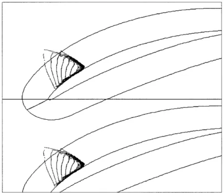
x/c

Figure 1-4: Perturbation velocity vectors during passage of a density wake of width 0.2c and density ratio 0.5 through the NACA4F blade row. The flow is inviscid and incom-pressible. r = 0.65.

the blade row during passage of the density wakes. This local reduction in ACp is a re-sult of the low density fluid directed toward the blade suction surface5. The perturbation velocity vectors plotted in Figure 1-4 clearly indicate this fluid motion and the associated counterrotating vortex pairs6.

The corresponding fluctuation in the blade azimuthal force coefficient Cy and moment coefficient Cm (about the blade mid chord) is shown in Figure 1-5 for a range of density wake widths and density ratios. Initially a reduction in the azimuthal force occurs as the density wake convects over the front half of the blade. This is followed by a gradual return to steady state as the density wake leaves the blade trailing edge. Similarly an increase in the counterclockwise moment occurs as the density wake convects over the front half of the blade. As the density wake passes the blade mid chord, the moment decreases back towards steady state. The shape of these force and moment profiles are roughly common over the

5

Further discussion can be found in Chapter 4.

6It can be argued that the induced velocity field of the counterrotating vortices direct the density wake fluid to the blade suction surface. No clear distinction can be made between cause and effect however. Both events (fluid flow and counterrotating vortices) occur simultaneously.

-0.08 -0.1 -0.12 -0.5 0.02 0.01 - 2/P '=0.5, w/c=O.1 \ - p₂/pl=0.5, w/c=0.2 "- - p2/ p = 0.8, w/c=0.4 0 0.5 1 1.5 Time

S,,-p2

p1=0.5, w/c=o.1

Figure 1-5: Fluctuation in (a) azimuthal force coefficient and (b) moment coefficient (positive counter-clockwise about the mid-chord) during passage of density wakes. ACy = Cymax - Cymean, ACm = Cmmax - Cmmean where Cymean = 0.75, Cmmean =

-0.13. Reproduced from Ramer.

range of density wake widths, 0.1 < w/c < 0.4, and density ratio's 0.25 < P2/P1 < 2.0 studied. The maximum change in the force and moment coefficients as functions of wake width and Marbles density parameter p* are plotted in Figure 1-6 and Figure 1-7.

The amplitude of the maximum fluctuations in the force and moment coefficients were found to scale linearly for small wake widths w/c and small density parameter p*. This scaling is given by,

CYmax - Cymean = 2.19 CYmean Cmmax - COmmean Cmmean (1.4) (1.5) = -3.05 - * c

0.3 , 0.2 0.1 0 Acy -0.1 -0.2 -0.3 -0.4 _ -0.8 -0.6 -0.4 -0.2 0 0.2 0.4

Figure 1-6: Maximum fluctuation in the azimuthal force coefficient (from ing passage of density wakes through the NACA4F blade row. Cymean)/Cymean. Reproduced from Ramer.

ACm=MO+M1*p*+M2*p*2 0.08 0.06 0.04 - -0.02 -ACm 0 -0.02- w/c--O.1 -0.04 -- - w/c=0.2 -- , - w/c=0.4 -0.06 -0.08

steady state) durACy = (Cymaz

--0.8 -0.6 -0.4 -0.2 0 0.2 0.4

Figure 1-7: Maximum fluctuation in moment coefficient (from steady state) during passage of density wakes through the NACA4F blade row. ACy = (Cyma - Cymean)/Cymean. Reproduced from Ramer.

1.4.1

Conclusions Based on Inviscid Results

1. The controlling flow feature responsible for the density wake induced blade force and

moment fluctuations in inviscid incompressible flows is the flow of density wake fluid by the action of centrifugal forces. During passage of a low density wake the wake fluid is directed toward the blade suction surface. This low density fluid reduces the blade force coefficient and increases the counter-clockwise moment coefficient. The opposite is true for a wake with higher density than free stream. In this case the density wake fluid is directed toward the blade pressure surface.

2. The shape of the force and moment coefficient fluctuations are common over the range of density wake widths 0.1 < w/c < 0.4 and density ratios 0.25 < p2/P1 < 2.0 considered.

3. Parametric studies show the amplitude of the maximum fluctuation in blade force and moment coefficients to have the following functional relationship:

ACy = f(w/c, p*, Cy(mean)) ACm =

f

The effect of blade spacing h/c is included in Cy(mean) and Cm(mean).

4. For w/c < 0.2 and -0.2 < p* < 0.2, ACy and ACm scale linearly. Increasing non-linearity is observed for larger wake widths and density ratios.

For further discussion of the inviscid results see Ramer [19], Ramer [21] and Wi-jesinghe [24]. Details of the inviscid flow solver and computational grid can also be found

in Ramer [19].

1.5

Questions Posed by the Current Research

Prior research on density wake induced blade force and moment fluctuations have been restricted to the case of inviscid incompressible background flows. These assumptions do not hold near blade surfaces and at high speeds typical of turbomachinery fans and compressors where boundary layers and blade passage shock waves could be significant. Furthermore it is unclear whether the functional relationships and parametric variables governing density

wake induced force and moment fluctuations in inviscid incompressible flows are applicable to viscous compressible flow environments. The following questions are posed to address this problem:

1. What are the additional controlling fluid dynamic features responsible for the blade force and moment fluctuations in viscous compressible background flows ?

2. What additional scaling parameters (if any) besides density wake width and density parameter p* are required to quantify the blade force and moment fluctuations for a given Mach number ?

3. What are the parametric trends in force and moment fluctuations with increasing free stream Mach number ?

The answers to these questions will help characterize the density wake induced forces and moments to a more broader realistic range of flow environments.

A key obstacle to HCF prevention alluded to earlier is the difficulty to formulate general guidelines which can provide a bound on the maximum fluctuating forces and mo-ments. This is due to the high dimensionality of the parameter space that must be investi-gated. A simple model which can accurately predict this boundary economically with low expenditure in time and cost will be of value to the design process. To help initiate the development of such a model the following questions are posed:

1. Can a simple physical flow model be developed from the CFD results to determine the trends in the blade force and moment fluctuations ?

2. If so can this model be used to predict trends in force and moment fluctuations for a wider range of cascade geometries and density wake properties ?

1.6

Technical Approach

Computational fluid dynamics (CFD) is the "tool" used in this research to investigate the forces and moments induced by convecting density wakes in viscous compressible

back-ground flows. CFD is a relatively inexpensive and convenient method to investigate flow phenomena compared to experimental investigations in wind tunnels. In particular the flow field properties at any location in the computational domain can be conveniently determined and an overall "picture" of the flow can be generated to help identify specific flow features. The flow geometry and free stream conditions are also easily changed within a CFD simu-lation compared to an experimental facility where arbitrary changes in flow geometry are generally not feasible.

The use of CFD is constrained by available computational resources however. This research has therefore been limited to two-dimensional unsteady flows with a single com-pressor blade row geometry. While turbine blades are subjected to larger density non-uniformities (due to hot-streaks from the combustor and from blade cooling), compressor blades are considered here since they are more susceptible to HCF failure.

The density wakes considered convect along the axial direction and have density gradi-ents directed only in the axial direction. Discussion is focused on low density wakes (wake densities lower than free stream density) which are more common in compressor blade pas-sages. To help isolate individual flow features a single density wake is convected through the blade passage in all simulations. The density variation inside the density wake is specified to be sinusoidal. This variation is considered to be a representative case.

To address the issue of the feasibility of a physical model to investigate the wide pa-rameter space of density wake - cascade blade row interactions a simple cascade model is developed. The model uses a combination of singularity solutions and a proportional constant determined from the inviscid CFD results.

1.7

Thesis Contributions

The aim of this research has been to contribute towards the "aerodynamic vibration forcing prediction" aspect of the high cycle fatigue problem. In this regard convecting density wakes were identified as a possible sources of high cycle fatigue failure. The density wake induced blade force and moment fluctuations were characterized for viscous compressible background flows with flow Mach numbers ranging from M. = 0.15 to M = 0.87. The

important contributions from this thesis can be listed as follows.

* The magnitude of the force and moment fluctuations in viscous compressible flows were quantified for,

1. Density wake widths w/c = 0.1, 0.2, 0.4, 1.0

2. Density ratios P2/P1 = 0.25, 0.50, 0.75, 2.00.

3. Flow Mach numbers M, = 0.15, 0.53, 0.63, 0.87.

* The force and moment fluctuation magnitudes in viscous compressible flow are found to scale with (1) the non-dimensional density wake width w/c and (2) Marble's density parameter p* for a given Mach number. The force and moment fluctuation mgnitudes also increase with flow Mach number. The maximum fluctuation in the azimuthal force coefficient in particular was found to scale with the Prandtl-Glauert compress-ibility factor /1 - M2 for small density wake widths (w/c = 0.1). The Prandtl-Glauert factor does not adequately scale the axial force coefficient or the moment coefficient however. Additional compressibility scaling relations are required for these coefficients.

* The baseline viscous compressible background solutions obtained prior to introducing density wakes have uncovered "self-excited" blade force and moment fluctuations due to periodic vortex shedding at the blade trailing edge. The vortex shedding induced force and moment fluctuations have amplitudes up to +13% from the time averaged mean values. This is a possible additional source for HCF failure.

* The density wake - boundary layer interaction was found to generate a separation bubble on the blade suction surface which causes additional blade force and moment fluc-tuations. The amplitude of these additional fluctuations scale with the maximum