Derivation of Internally-Consistent Thermodynamic Data by the Technique of Mathematical Programming: a Review with Application the System MgO-SiO2-H2O

(1)

Derivation of Internally-Consistent Thermodynamic

Data by the Technique of Mathematical Programming:

a Review with Application to the System

MgO-SiO

2

-H

2

O

by R. G. BERMAN,1 M. ENGI,2 H. J. GREENWOOD,1 AND

T. H. BROWN1

1 Department of Geological Sciences, University of British Columbia, 6339 Stores Road, Vancouver, B.C., Canada V6T 2B4

2Institut fur Mineralogie und Petrographie, ETH-Zentrum, CH-8092 Zurich, Switzerland (Received 9 October 1985; revised typescript accepted 17 June 1986)

ABSTRACT

The problem of deriving an optimal set of thermodynamic properties of minerals from a diverse experimental data base is reviewed and a preferred methodology proposed. Mathematical pro-gramming(MAP) methods extend the linear programming (LIP) approach first presented by Gordon (1973), and make it possible to account for the type of information conveyed, and the uncertainties attending both phase equilibrium data and direct measurements of phase properties. For phase equilibrium data which are (in most cases) characterized by non-normal error distributions across experimental brackets, the midpoint of a bracket is no more probable than other points, and the data are best treated by considering the inequality in the change in Gibbs free energy of reaction at each half-bracket. Direct measurements of phase properties can be assumed to have approximately normal error distributions, and the MAP technique optimizes agreement with these values by using the principles of least squares in the definition of an objective function. The structure of this problem, treatment of uncertainties in various types of experimental data, and method of optimizing final solutions are discussed in some detail.

The method is applied to experimental data in the MgO-SiO2-H2O system, where inconsistencies

among the data are resolved and an optimal set of thermodynamic properties is presented. The derived standard state entropies and volumes agree with all direct measurements (within their uncertainties), as do enthalpies of formation from the elements except for those of talc (+16 kJ mol" •), anthophyllite (+ 14 kJ mol~'), and brucite (— 1 kJ mol~'). Stable phase relations in the system have the topology predicted by Greenwood (1963, 1971), with quartz- and forsterite-absent invariant points at 683 "C-6-4 kb and 797 °C-12 kb respectively, repeating at 552 °C-120 b and 550 °C-55 b. The thermodynamic analysis indicates little remaining flexibility in the phase relations, which, when combined with suitable activity models for solid solution, should allow for accurate determination of the conditions of metamorphism of ultramafic rocks.

I N T R O D U C T I O N

Modern petrology has come to depend more and more heavily upon computed equilibrium relations among minerals and solutions. The need is felt equally by both experimental petrologists and by those whose data and problems come from natural assemblages. This need to compute equilibria has sharpened the demand for thermodynamic data that are both comprehensive and internally consistent, i.e. that agree with all the primary experimental data.

(2)

1332 R. G. BERMAN ET AL.

Information yielding thermodynamic data is acquired chiefly in two distinct ways. The first and classically standard approach is through calorimetric measurement of individual phase properties, and the second consists of determination of equilibria between assemblages of phases. The latter, while dealing directly with some of the equilibria of interest, does not determine any thermodynamic property of any individual mineral, but only changes in the thermodynamic properties of the reaction. The two are related, however, by the fact that these 'delta' properties can all be derived through linear combinations of the properties for the individual phases. A satisfactory technique of thermodynamic analysis must evaluate data from both sources, as well as data pertaining to heat capacity and molar volume. In addition, there is a need to incorporate a growing body of data that involves minerals which exhibit solid solution behaviour and/or ordering phenomena.

Several compilations of calorimetric data for minerals are in use at present, including those by Kelley (1960), Kelley & King (1961), Robie et al. (1979), Stull & Prophet (1971), and CODATA (e.g., 1978). Important differences between these notwithstanding, they all are similar in that they make little use of constraints from phase equilibrium data. It has been pointed out, however, that consideration of mineral equilibria can considerably refine values determined calorimetrically (Zen, 1972). For example, typical uncertainties in calorimetric-ally determined enthalpies of formation are 1-5-6 kJ mol"1, whereas the width of a phase

equilibrium bracket may translate to as little as 1-2 kJ mol"1 distributed among all the

phases in the equilibrium. For this reason, petrologists have increasingly turned to phase equilibrium data for their fine-tuning of thermodynamic parameters.

Although several different techniques have been employed for the extraction of thermo-dynamic parameters from phase equilibrium experiments, all are founded on the same principle, namely, that the stable assemblage is the one with the lowest free energy. Consequently, all we can deduce from a successful phase equilibrium experiment, in which one assemblage is observed to be more stable than another, is the sign of the free energy change. No other information is available. In particular, there is no information on where, within a reversed bracket, the equilibrium conditions might lie. There exists no 'central limit theorem' to favour the mid-point of a bracket, and no way to say how far from a 'half-bracket' the equilibrium might lie. This non-central characteristic of such experiments was first recognized by Gordon (1973, 1977), who introduced the technique of linear programming (LIP) to the literature of experimental petrology. Briefly, LIP is a mathematical technique for analysis of systems of linear inequalities which, in the case of phase equilibrium data, express the sign of the free energy change of an experimentally observed reaction. The first step of the solution involves establishing the existence of a 'feasible region' that is consistent with all inequality constraints, while the last step uses an objective function to maximize or minimize any variable or linear combination of variables. Following Gordon's lead, the linear programming approach has been applied in several studies, including those by Day & Halbach (1979), Day & Kumin (1980), Hammerstrom (1981), Halbach & Chatterjee (1982,

1984), Berman & Brown (1984), and Day et al. (1985).

Others have used techniques more recognizable to statisticians such as multiple linear regression (Zen, 1972; Haas & Fisher, 1976; Haas et al, 1981; Robinson et al., 1982; Powell & Holland, 1985), in which the statistical 'central tendency' was controlled by various schemes of data weighting (Haas et al., 1981; Lindsley et al., 1981). The most extensive published analysis to date is that of Helgeson et al. (1978), which used a method of successive fits to experimental data in progressively more complex systems. Each new item of data added to the compilation was required to agree with thermodynamic properties of phases that had been fixed by previous analysis of experimental data, an unsatisfactory method because 'best fit' curves are not required to be consistent with all brackets, the derived properties depend

(3)

THERMODYNAMIC DATA 1333 TABLE 1

Comparison of LIP/MAP and regression techniques for the analysis of phase equilibrium data

Linear programming analysis Regression analysis

Treats phase equilibrium data as statements of inequalities in Ar G

Analyses individual half-brackets

—provides for constraints from unreversed experi-ments

—every half-bracket can be analysed with different assumptions (e.g., solid solution effects, different starting materials)

Ensures consistency with all data (if consistency is possible)

Provides a range of solutions (feasible region) from which a unique solution is obtained with a suitable objective function

Uncertainties approximated by the range of values consistent with all data

Treats weighted midpoints of brackets as positions where Ar G = 0

Analyses pairs of experimental half-brackets

Minimizes sum of squares of residuals, but does not ensure consistency with all data

Provides a 'unique' solution (dependent on weighting factors)

Uncertainties computed from variance/covariance matrix

on the order of data analysis, and not all experiments that involve a given phase contribute to the refinement of its thermodynamic properties.

There seems to have developed something of a schism between those who prefer the well-tried methods of multiple linear regression and those who prefer to apply the technique of linear programming to the analysis of phase equilibrium data. The purpose of this paper is, in part, to set out clearly the differences between the two methods, and to argue that the linear programming method, or a non-linear variation of it, is more powerful than regression analysis, largely because it provides a mathematical technique that is compatible with the nature of phase equilibrium data. Differences between the two techniques are summarized in Table 1 and discussed in the following pages. The essential difference can be appreciated by considering a pair of experiments which bracket a given equilibrium. Regression operates on the pair of half-brackets and produces a solution that is controlled by, but not (necessarily) coincident with, the midpoint of the experiments. LIP operates on individual half-brackets, and produces a solution consistent with the directional sense of each half-bracket, but which may lie at any point between the experiments. The significance of this difference is that, in an analysis of favorable sets of experimental data (i.e. those for which it is possible to obtain solutions that do not conflict with any experiment), LIP ensures consistency with all half-brackets, while regression analysis may contradict individual data points in the process of achieving a statistical 'best fit' to the weighted midpoints. This difference becomes increasingly important as the number of experimental brackets grows and the opportunity for inconsistencies among the data increases. Clearly, any analysis that purports to produce a 'best fit', and yet contradicts valid data, is not optimal.

It can also be argued on the basis of statistical treatment of the errors associated with phase equilibrium data that regression is not an appropriate means of analysis for these data. Demarest & Haselton (1981) showed that normal error distributions are associated only with those data for which d/s < 1, where 2d is the temperature separation between half-brackets and s is the standard error of reported temperatures. Although s is seldom documented, and is difficult to assess from the information commonly reported by experimental petrologists (c.f. Bird & Anderson, 1973), reasonable estimates indicate that d/s is commonly in the range 2-4. For such data, the probability distribution is constant across the central portion of a bracket, and the midpoint of the bracket is no more probable than any other point.

(4)

1334 R. G. BERMAN ETAL.

Regression techniques are appropriate, however, for the analysis of calorimetric and volumetric data because these measurements can be assumed to be governed by a Gaussian error distribution, with the mean value being the most probable. The technique of LIP can be modified to take account of this fact by using a non-linear objective function that applies the least squares criterion to these data. Thus, the method of deriving thermodynamic properties which we discuss in this paper takes into account the nature of the uncertainties attending each type of data used in the analysis.

We define an optimal set of thermodynamic properties by the following two criteria, first in words and more formally below. An optimal set of properties is characterized by: (1) Thermodynamic consistency with all valid experimental constraints, be they independently measured properties of a phase or indirect constraints from phase equilibria. (2) Minimum deviation, in the least-squares sense, of derived parameters from their directly measured values.

Mathematical programming (MAP) methods, which include a variety of optimization techniques of which linear programming is one, are used for the data analysis.* These techniques are not dealt with in this paper, as numerous texts cover the topic (e.g., Himmelblau, 1972; Gill et al, 1981). In the following pages we provide details of the mathematical programming approach, which in part reiterate, and in part extend the lucid presentation of LIP techniques by Halbach & Chatterjee (1982). The order of presentation follows the order of most general solution algorithms. We first discuss the constraints from which a feasible solution is obtained, and show how to incorporate uncertainties in the data used to formulate these constraints. We then discuss the objective function that defines optimal values of all parameters using least squares criteria while maintaining the consistency achieved in the first step. Lastly, we show an example of the method with an analysis of experimental data in the system Mg0-SiO2-H2O.

CONSTRAINTS ON THE SOLUTION

Calorimetric constraints

Calorimetric and volumetric data directly constrain standard-state thermodynamic properties (Af H°, S°, V°) of individual minerals. As most data are reported with two sigma

uncertainties (Robie et al., 1967,1979), these uncertainties can be used to bracket a measured value, using upper and lower 'bounds' provided with most LIP/MAP software packages. These bounds ensure that solutions will be within the uncertainties of these data, and 'best' values can be derived in final optimization of the problem discussed below.

Although this procedure is straightforward in principle, several difficulties are commonly encountered. For third law entropies, only the lower bound can be used if a zero-point contribution for disorder of unknown magnitude is required for a given phase. For many * The alternative method to MAP that has been addressed above is commonly termed unconstrained regression

analysis, whether linear of nonlinear. It is this technique that has been used to date by proponents of regression

analysis for the problem outlined here (Helgeson et al., 1978; Haas et al., 1981). There exist, however, constrained

regression methods that allow incorporation of a (limited) number of constraints on the fit parameters (see e.g.,

Lawson & Hanson, 1974). Typically, such least squares problems are solved by algorithms which proceed in the reverse direction to MAP routines, in that they first solve the unconstrained problem. The initial solution is subsequently modified by means of one or more suitable strategies aiming at reducing iteratively the inconsistencies with the parameter constraints. If successful, one would expect such algorithms to produce optimal and consistent solutions very similar to those obtained by MAP techniques and, at least in theory, the distinction between the two methods becomes immaterial. We are not aware of any practical attempt to use constrained regression techniques to solve an optimization problem of the size and structure outlined here, although a recent application (Ghiorso

et al., 1983) makes use of specially designed regression routines to calibrate thermodynamic properties for

(5)

THERMODYNAMIC DATA 1335

minerals, various precise molar volume determinations do not overlap within the stated uncertainties. Unless one value is preferred (because, for example, of sample purity or superior phase characterization) a practical solution is to use bounds which span the entire range of values and associated uncertainties. The most difficulty arises with enthalpies of formation, which show a great deal of scatter between different determinations (e.g. Af HfOrsterite summarized in Table 3), and calorimetric values for many phases are not

consistent with phase equilibrium data (Berman et al., 1985). We have found it most convenient to establish reference values by placing bounds on the Af H° value of only one

phase for each component in the system under analysis, and then use the final optimization to achieve consistency with as many other measured enthalpies as possible.

Phase equilibrium constraints

Phase equilibrium data are characterized by measured pressure, temperature, and phase composition. In some sets of data, phases are of variable composition, and in some the activities of one or more species may be controlled. Regardless of the variables that have been measured, the basic thermodynamic information gained from conversion of phase assemblage A to assemblage B under the static physical conditions of an experiment may be cast into an inequality in Gibbs free energy:

GA > GB (1)

or, equivalently,

GB- GA< 0 . (la)

In general,

Ar GFT <0 (products stable) (2a)

Ar GPT >0 (reactants stable) (2b)

where Ar Gp'T is the Gibbs free energy of a reaction at pressure, P, and temperature, T (Kelvin). These relations are independent of any reference state. The change in free energy of a reaction is computed from:

phases

ArGPT = I ^KGPT (3)

i

where Vj are reaction coefficients, and Aa GPl r is the apparent Gibbs free energy of formation (Benson, 1968; Helgeson et al, 1978) of phase i from the elements at P and T. Adopting as the standard state the pure phase at P and T, this can be expanded by:

AaG fr = AaHPT-TSPT + RT\nai (4)

where at is the activity of i,

(5)

T, P,

and, if volume is considered to be independent of T,

(6)

S° and Af H° are the third law entropy and enthalpy of formation from the elements, = S

(6)

1336 R. G. BERMAN ETAL. TABLE 2

Separation of variables for the mathematical programming problem (relation 8)

Left hand side Right hand side

(LHS) (RHS) Assumptions/equations for evaluation of RHS

T

AfH° j C p d T For minerals: Berman & Brown (1985); for aqueous

Tt species: H e l g e s o n et al. (1981)

T

S° - T - J ( C p / T ) d T For minerals: Berman & Brown (1985); for aqueous

jt species: Helgeson et al. (1981) p

V° j(VPiT—V)dP Assumed equation of state for minerals and aqueous

Pi species

p

| Vt,,dP Assumed equation of state. For H2O: Haar et al. P (1984), Delany & Helgeson (1978); for CO2: Kerrick

& Jacobs (1981)

RT In a, X-, known from experiments; y, = 1 (ideal), or calculated

with an assumed model

respectively, both at the reference pressure (PT = 1 b) and temperature (Tr = 298-15 K). Combining equations 3-6 gives

phases T T P

AIGPT=

£ v

i

{A

f

#°-r-s°+JCp,dr-r-j(Cp/r)dr+Jv;d/'+/mna

i

}. (7)

' T, T, P,

Each phase equilibrium experiment provides an inequality constraint (relations 2a or 2b) which, when expressed through equation 7, involves a rather large number of parameters, consisting of the experimental variables and the thermodynamic properties of all phases. Mathematical programming (MAP) techniques require that we separate all terms into two classes. The first class includes all terms with parameters to be determined, which are collected on the left hand side (LHS) of the inequalities 2a or 2b. The second class includes all terms that are thought to be known sufficiently well to be treated as constants, and are therefore collected on the right hand side (RHS). Table 2 shows a convenient separation of variables, along with the assumptions and equations that we have used to evaluate them. At the pressure and temperature of each experiment, the sum of the terms on the RHS is a constant, C. Combination of equation 7 with relations 2a and 2b then yields

phases minerals

X vi{Aff/?-T-S?}+ X Vi{K?(P-Pr)} < C (products stable) (8a)

i i

" f " vi{Af H° - T• S?} + """IfS v;{ V?(P - Pr)} > C (reactants stable). (8b)

i i

The relations given in 8a and 8b are linear in the variables (Af H°, S°, V?), and represent

the fundamental equations by which standard state thermodynamic properties of minerals (or any other phase or species) can be derived from phase equilibrium data by means of mathematical or linear programming. We have found that the separation of variables shown in Table 2 generally allows for more than adequate solutions to large problems (Berman et

al., 1985). Thus, prior to the MAP analysis, CP functions of all minerals (and expansivity/

(7)

analysis of relevant data, and equations of state for gases and aqueous species are adopted. If volumetric or calorimetric data are not available for certain minerals, or if such data are of questionable accuracy, the appropriate coefficients can be left as variables on the LHS of the MAP problem. In such cases constraints on these properties are needed to ensure reasonable solutions, and a technique for providing these constraints is discussed below under 'The Objective Function' section.

In analysis of phase equilibrium data involving solution phases, all activity terms can be grouped on the RHS (as shown in Table 2) if compositions of all phases are known and activity models are adopted. In many cases, it may be preferable to derive solution parameters at the same time as standard state properties (e.g., Berman & Brown, 1984; Engi

et al., 1984). Activity terms for all phases can then be factored (RT In a = RT In y + RT In X)

such that the RTlnX terms remain on the RHS, while all parameters used to represent the

RTlny terms are moved to the LHS. Depending on the functional form chosen to describe

the latter terms, the constraint relations may be linear in all parameters or in all but a few solution parameters (W), as long as compositions of all solution phases are known or can be estimated. For example, Berman & Brown (1984) presented a generalized form for Margules equations and showed that they yield linear constraints on the interaction parameters which can be solved with the method of LIP. Other formulations, such as the quasi-chemical or the van Laar equations, contain nonlinear terms because the interaction parameters cannot be factored so as to be solely functions of compositional variables. In such cases, solution of the problem requires mathematical programming techniques to analyse these nonlinear constraints.

While exchange equilibrium data are also treated as discussed above, it may be useful to comment further on the derivation of the sense of the inequality sign in (2), which depends on the directional sense of the reaction observed experimentally. For standard reversal experiments, this directional sense derives from the observed changes in phase proportions between initial and final run charges. For exchange equilibria, the directional sense stems from the observed changes in phase compositions. Thus, relation 2a (products stable) applies if one can show that in the course of an experiment the composition of all solution phases changed such that the phase components on the right hand side of an expressed equilibrium increased, while those on the left hand side decreased. Relation 2b (reactants stable) holds if the solution phases show the opposite sense of compositional changes.

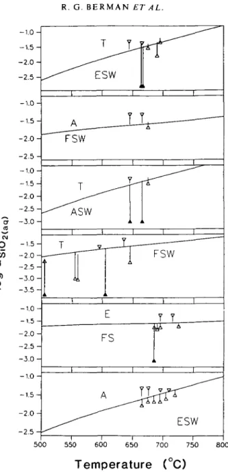
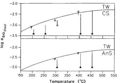
It is also important to note that the structure of the problem described above applies equally well to solubility experiments, although we are unaware of previous attempts to analyse such data with LIP or MAP techniques. In most solubility experiments, such as

quartz = SiO2(aqueous) (9)

the progress of a reaction is monitored by tracing the changes in fluid composition. Experiments in which equilibrium is approached from undersaturation involve quartz dissolution, and they yield half-brackets for which relation 2a (products stable) holds. Experiments in which equilibrium is approached from supersaturation yield half-brackets for which relation 2b (reactants stable) holds. When equilibria have not been reversed, but experiments have been run for a sufficiently long duration to expect that equilibrium was obtained, it may be appropriate to add an 'artificial' constraint which provides the opposite half-bracket for the equilibrium.

TREATMENT OF EXPERIMENTAL ERRORS IN PHASE EQUILIBRIUM DATA In the case of two experiments that bracket an equilibrium, there is a probability of 10 that the equilibrium lies between the experimental data points (e.g., Zen, 1972; Demarest &

(8)

1338 R. G. BERMAN ETAL.

Haselton, 1981). Any intermediate point is equally likely as the location of the equilibrium conditions. However, the nominal conditions reported for an experiment may not coincide with the actual conditions because of unavoidable errors in control and measurement of run conditions. Thus, to ensure certainty that the equilibrium conditions lie between the conditions used in the data analysis, it is essential to use not the nominal values, but adjusted values that account for the experimental uncertainty in defining the conditions of the experiment. Specifically, the brackets must be expanded to the limits allowed by the combined uncertainties in control and measurement so that they are less constraining than the nominal values. In this way we may be certain that the true equilibrium lies between the points used in the data reduction. If, after such adjustment, an experiment is inconsistent, we must look to other causes such as insufficient reaction progress, inadequate phase characterization, inappropriate equations of state, or unreasonable estimates of experimental accuracy and/or precision. Consequently, it is important that the magnitude of the errors reported by an experimentalist account for both the experimental precision (arising from P-T fluctuations during a run) and for the accuracy (which incorporates uncertainties resulting from calibration, temperature gradients across samples, etc.). Insufficient reaction progress or incomplete characterization of any phase introduce doubt as to the validity of the experiment, rather than numerical contributions to the precision or accuracy.

In general, the P-T-X coordinates of experimental data should be adjusted in such a way that the adjusted data form the widest permissible brackets for the equilibrium. Proper treatment of experimental brackets thus requires knowledge of the slopes of the equilibrium curve with respect to all intensive variables. The nominal value, /, of each variable controlled during an experiment is adjusted to

I* = I + E A , (10)

where /* is the adjusted value, E is the error (best estimate of the combined precision and accuracy) in this variable, and A, takes the value + 1 or — 1, as described below. For a given bracket on the high or low temperature side of an equilibrium (/ = T), AT is equal to + 1 or

— 1, respectively. A, for other variables is given by

A, = Astab-Aslope (11)

where Aslab takes the values — 1 or + 1, depending on whether the high or low temperature

assemblage is stable, respectively, and As,ope takes the value + 1 or — 1 corresponding to the

sign of the (dljdT) slope of the equilibrium. In most cases the relevant (81/dT) slopes are known from the phase equilibrium data, but where the slopes are uncertain and thermodynamic variables are reasonably well known, they can be computed from the thermodynamic relations: (dP/dT)x c = 0 = Ar5/Ar V, (dT/dXj)P G = o = (RT)/(Xj ArS), and (dP/dXfa c = o = -{RT)/{XS Ar V). '

Reversal experiments

In reversal experiments, each experimental charge has the potential to yield one half-bracket for an equilibrium. The directional sense of the half-bracket is determined by growth of one assemblage and reduction of another from starting materials that contain either reactants, products, or a mixture of both. The most important requirements in assessing the reliability of such experiments are: (1) that phases are suitably well characterized with respect to composition, ordering state, grain size, etc.; (2) that the amount of reaction observed is sufficient to establish the direction of reaction with confidence; and (3) that changes in the proportions of all phases are consistent with the reaction stoichiometry

(9)

650 660 670 680 690 700

Temperature (C)

710

FIG. 1. Method used to derive the pressure and temperature of data points for MAP analysis (triangles) from nominal experimental half-brackets (squares) with P and T uncertainties shown by error bars. Note that the adjustment to account for experimental uncertainties must take into account the slope of the equilibrium curve (see

text).

without the appearance of extraneous phases, so that one is certain of the reaction for which data have been collected.

For reversal experiments in which all phases are of fixed composition, the method of adjustment for experimental errors is straightforward (Fig. 1). Because many dehydration reactions change from positive to negative slope with increasing pressure, care must be taken to adjust brackets with the appropriate slope. Thus, preliminary calculation of the equilibrium curve may be necessary to ascertain the region of slope change, although the actual value of the slope is not needed in the adjustment. Care must also be taken in adjusting data for equilibria evolving H2O and CO2 which exhibit maxima in the T-XCO2 plane.

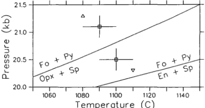
It seems worthwhile to point out that use of MAP or LIP techniques allows the incorporation of some constraints from experimental data involving a solution phase even when an activity model for a solution phase is not known or assumed. For example, if the model is not known, and we have a pair of half-brackets on the equilibrium forsterite (Fo) + pyrope (Py) = orthopyroxene (Opx) + spinel (Sp) (Fig. 2), the half-brackets in the 'Fo + Py' field place valid constraints on the thermodynamic properties of stoichiometric enstatite because enstatite must have a smaller stability field than the stable aluminous

21.5 21.0 -v_ 13 2 0 . 5 -CD CL 20.0 1060 1080 Temperature (C) 1140

FIG. 2. MAP analysis applied to experimental half-brackets for an equilibrium involving a solution phase (Opx). The low pressure experiment must be analysed in conjunction with a solution model for Opx, whereas the high pressure half-bracket is a valid constraint for the equilibrium involving Opx as well as stoichiometric enstatite (En). This is true because the equilibrium with En must lie at lower pressure than the displaced equilibrium with stable

(10)

orthopyroxene. The same argument more commonly applies when a solution model is used, but when we are not certain that a given phase has attained its equilibrium composition. If, for example, the starting materials for an experiment of short duration on the above equilibrium contained stoichiometric enstatite, it is often preferable to use stoichiometric enstatite for the 'Fo + Py stable' half-bracket, and the stable orthopyroxene composition for the 'En + Sp stable' half-bracket, rather than assume that the equilibrium orthopyroxene composition was attained.

Weight change experiments

Several studies monitor reaction progress by weight changes in isobaric series of experiments, spanning a range in either temperature (e.g., Evans, 1965) or fluid composition (e.g., Jacobs & Kerrick, 1981). Such experiments permit the determination of phase equilibrium boundaries by extrapolation of the monitored weight or composition changes to the line of zero weight or composition change. These data can be analysed with MAP techniques by creating half-brackets that reflect the experimental uncertainties in location of the equilibrium. In evaluating the existing data from weight change studies, we have observed a surprisingly high proportion of inconsistencies. These are particularly common in studies monitoring fluid composition (e.g., mole fraction ZC OJ, even though the experiments

themselves appear to have been performed carefully. Scrutiny of the reported procedures leads us to propose two likely sources for the disagreement: (a) the experimental uncertainty of each data point is commonly neglected when the locus of equilibrium conditions is determined; and (b) the functional form fitted to the raw data has no theoretical basis and may be inadequate.

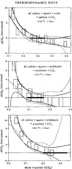
Consider, for example, three data sets (Fig. 3) on two decarbonation reactions studied by Jacobs & Kerrick (1981). These authors calculated equilibrium XCO2 values and their uncertainties by fitting the experimental data to an arbitrary polynomial quadratic in XCOl, ignoring: (a) the experimental errors in XCOl and ACO2 (the number of moles of CO2

consumed/produced in an experiment); and (b) the possibility that alternate functional forms chosen to represent the data might yield an intercept at a different XCOr Until a functional form derived on the basis of kinetic theory becomes available, point (b) may be best evaluated by fitting the same experimental data sets to alternate arbitrary functions chosen with the intent to represent the data locally, near ACO2 = 0.

We have investigated the combined effects of points (a) and (b) for the data reported by Jacobs & Kerrick (1981) using a Monte Carlo approach to estimate the uncertainty in XCO2 at ACOl = 0. The raw data were perturbed by U*R, where U denotes the reported experimental uncertainty ( + 001 in XCO2 and + 1 fimol in ACO2) and R denotes a random number. For each

data point, one thousand such numbers were generated, having a standard deviation of 1 and a mean of 0. For each set of perturbed data, a least squares fit was computed. In addition to the quadratic polynome used by Jacobs & Kerrick, alternative polynomes were tried, involving terms in (XCO2)~l and (ATC02)4. Figure 3 displays some representative confidence

bands resulting from these calculations. These figures illustrate several important conclu-sions about the potential hazards in the interpretation of weight change data:

1. As long as the functional form to fit weight change data is not known theoretically, it is not sufficient to represent the data by one type of polynomial. Several functions should be tested and compared, both against the raw data and with respect to their behaviour near zero weight change. In many cases, the error brackets indicated by such a procedure are considerably wider than would be apparent from fitting to only one functional form.

2. For data sets that do not significantly cover regions on both sides of the equilibrium, only one half-bracket can be defined with confidence.

(11)

T H E R M O D Y N A M I C D A T A 1341

a) calcite + quartz + rutile - sphene + CO2

1450 °C, 2 kbar)

0.3

\\| b) calcite + quartz + andalusite - anorthite + CO2 (370 °C, 2 kbar) 0.2 o 2 6 o £ o O 0 V.

V-.

i e ) calcite + quartz + andalusite ' - anorthite + C O2

(400 °C, 2 kbarl

\

Mole fraction (CO2)

FIG. 3. Weight change data for two equilibria at different pressures and temperatures. The raw data with rectangular error boxes, and the derived uncertainties in the equilibrium values of XCOl (solid bars on base lines) are

from Jacobs & Kerrick (1981). 2a confidence bands were computed from Monte Carlo analysis of regression curves fit to three polynomials:

ACQ, = a + bx + ex2 (shaded regions; function used by Jacobs & Kerrick)

ACQJ = a + bx + c/x (long-dashed line) Ac0] = a + bx + ex2 + dx* (dotted line)

where x = ^C O l

-For each diagram, uncertainties in the location of the equilibrium position are defined by the intersection of the AcOl = 0 line with the computed 2a confidence bands. Where data lie at Ac o, values that are significantly on both

sides of the zero base line (Fig. 3a), the bracket defined by two of the functions are in good agreement. Data collected on one side of the base line serve only to define a single half-bracket (XCOl — 0 2 in Fig. 3c) because confidence bands

for all functions fail to intersect the base line at high XCOj. The alternate functions used to represent the data set in

Fig. 3b indicate larger uncertainties in the equilibrium position than derived by Jacobs & Kerrick (1981), with two of the functions failing to define a bracket at high XCOl.

(12)

3. From a theoretical point of view, fitting the kinetic behaviour of the two half-reactions by one simple function is probably inappropriate, for the pertinent rate constants are likely to be quite dissimilar. The error estimates obtained from a Monte Carlo analysis such as we have conducted are therefore still somewhat optimistic. Furthermore their validity depends crucially on the estimates of experimental uncertainties being realistic, with account being made for possible systematic errors, due for example to the presence of additional volatile species (CH4, H2) contributing to the total weight change observed.

THE OBJECTIVE FUNCTION

The preceding discussion outlines the first portion of the LIP/MAP problem: the structure of the constraints and the considerations necessary to set up the constraint relations. The set of constraint inequalities is analysed for internal consistency by mathematical programming techniques (LIP if all constraints are linear), and unless some of the constraints are in mutual conflict, such a set of constraints defines & feasible region within parameter space, such that any set of parameter values (fit values) from within the feasible region satisfies all of the constraint relations. It is quite commonly the case that various sets of experiments for one or more equilibria are in conflict, and permit no values that are consistent with all data. In such cases, the inconsistencies must be resolved by either: (a) removing certain data from the experimental data base, usually on the grounds of incomplete phase characterization and/or amount of reaction detected; or (b) expanding the errors assigned to certain experimental data for which documentation of the source of errors is lacking or questionable; or (c) modifying any of the coefficients of equations used to evaluate the RHS (Table 2), particularly CP coefficients. To some it may seem to be a disadvantage of the LIP/MAP approach that

inconsistencies need be resolved during analysis. Although it is true that regression analysis will produce solutions to systems of inconsistent data, meaningful solutions will only be obtained if those obviously discordant data are removed and the remainder re-analysed (see, for example, the discussion on pp. 19-21 of Haas et al., 1981). Thus, inconsistencies can and should be resolved with either technique. We feel that it is advantageous to use a mathematical technique that requires this critical evaluation step, and see no way to avoid the exercise of judgement in screening which data are to be included in the analysis.

Once a feasible solution has been obtained, one requires a selection criterion or objective

function in order to define and find a unique 'best' solution. The simplest objective functions

are linear in the variables of the problem and might be formulated so as to find the maximum or minimum AfH° of a particular phase, or the maximum or minimum of a linear combination of AfH°, S°, and V° values for one or more phases.

The objective function we prefer is nonlinear in the variables of the problem, and was developed to take account of the specific nature of the data, namely that in most chemical systems there exist numerous measurements of the fundamental properties of phases, especially of their molar volumes, heat capacities, entropies, and heats of formation. The precision of these data is typically evaluated by the experimentalists reporting them and, except for the temperature-dependent CP, their representation by a mean value with an

estimated standard error is probably justified. To the extent that such a representation approximates a Gaussian error distribution with its mean equal to Zt and its standard deviation equal to s,, it may be desirable to derive the Yj parameters by using the principle of least squares in the definition of the objective function (F). Therefore, we minimize

parameters

(13)

where the summation includes those parameters for which 'direct' physical measurements exist (e.g., Af H°, S°, V°). The qualitative effect of using an objective function such as (12) is

that one obtains as close a match between fit parameters and physical measurements as is permitted by the phase equilibrium data. The function proposed by Day & Kumin (1980), which minimizes the sum of the absolute values of the differences, produces very similar results but has the disadvantage of describing a discontinuous probability function.

In practice, we have found that application of (12) yields quite satisfactory solution sets. The implicitly assumed normal probability distribution of the fit parameters has been checked by computing residuals. As one might expect, outliers (unexpectedly large deviations) occur more frequently for those types of data which result from complex, indirect measurement. The uncertainty of Af H° measurements is more difficult to assess than that of V° or S° data, a fact that is reflected in the residual distribution. For example, analysis of large

systems of data involving more than 70 minerals (Berman et al., 1985) has shown that, whereas most V° and S° data are fit within 2<r, Af H° values are commonly fit within 3-4<r with

a few much larger deviations with the low-temperature HF determinations. These observations, together with the wide scatter among different measurements of Af H° of

specific minerals (for example, forsterite, discussed below), indicate that calorimetric enthalpies are the least accurate of the various data types used to determine thermodynamic properties of minerals. For this reason, we advocate exclusion of highly discordant Af H°

values, a conclusion that may help to alleviate the ambiguity between the 'minimum deviation' and 'minimax deviation' solutions proposed by Day et al. (1985). Although there exist robust statistical methods (Huber, 1981) which are designed to accommodate such outliers and which thus may eliminate undue subjectivity in data screening, further work is needed to assess the practical consequences of such formulations.

A remaining shortcoming of the objective function (12) is that phase equilibrium data carry no weight in the final optimization. Although, as discussed above, there is no justification for striving to position equilibrium curves midway between phase equilibrium brackets, it is somewhat unsatisfactory that equilibria be coincident with data points that have been adjusted for their estimated maximum uncertainties. One way to avoid this situation is to add to each constraint row representing a phase equilibrium half-bracket a 'slack' variable representing the difference (in temperature, for example) between the position of the fit equilibrium curve and the experimental data point. These slack variables can be added to the terms in (12) with a penalty function, the value of which increases as the adjusted position of any experiment is approached (pertinent slack variable approaches zero), but which becomes negligible as the nominal position of each experiment is neared. The main difficulty in combining the two components of the objective function lies in the relative weighting of residuals from the calorimetric and phase equilibrium data. For small, favorable, or only loosely constraining data sets, the problem may not be severe, but for data sets as large even as that described in the second part of this paper, conflict between the two types of data is unavoidable. Until further work defines a means of distributing the weight between these two components of the objective function, we recommend use of (12) for the final optimization of thermodynamic variables.

Optimization of CP or V(P, T) terms

It is frequently desirable to derive CP, expansivity, or compressibility coefficients

during analysis of phase equilibrium data if these coefficients are poorly defined by direct experimental data, or when examining possible sources of inconsistencies among experimental data. These coefficients can be derived in the MAP problem by changing the

(14)

separation of variables (Table 2) so that they appear as variables on the LHS. The coefficients can then be optimized using an objective function, modified from (12) such that the Yx are the computed heat capacities (or volumes) evaluated at each temperature (and pressure) for which the Cj> (or volumetric) data (ZJ were measured or estimated. This objective function is extremely useful for producing small adjustments to heat capacity functions so as to allow consistency to be obtained with otherwise inconsistent phase equilibrium data (see part II below).

Optimization o/KD values from natural assemblages

Carefully evaluated natural KD data offer a valuable check on, and extension of experimental data for many silicates, oxides, and other mineral groups. It is very important, however, to apply stringent criteria to the selection of data. Close approach to exchange equilibrium has to be demonstrated through mineral analyses, and the P-T conditions of equilibration must be estimated with care as they are not known directly, in contrast with experimental constraints.

If one assumes that measured distribution coefficients, KD, represent equilibrium conditions, then one may stipulate that the derived parameters for the minerals depart as little as possible from values that predict these measured Ko values. If the statement 'depart as little as possible' is construed in the least squares sense, for example, these new constraints are most easily met by including them in the (nonlinear) objective function. The separation of terms is straightforward: at given P and T, the equilibrium constant K may be factored as

K = KD*Kr K is related to Ar Gp< T and the latter may be expanded according to (7). Adopting explicit solution models for the coexisting solution phases permits factoring of Ky in terms of solution parameters. These Ky terms contribute to the RHS constant of relations 8a and 8b, while KD remains as a LHS variable.

UNCERTAINTIES IN DERIVED THERMODYNAMIC PROPERTIES Directly measured thermodynamic properties have well characterized uncertainties (2<j errors are commonly tabulated) which are based on the precision of the measurements and the uncertainties of auxiliary data. The task of assigning errors to thermodynamic properties that have been derived from phase equilibrium data is a very different problem that has been addressed repeatedly (e.g., Chayes, 1968; Zen, 1972; Bird & Anderson, 1973; Helgeson et al., 1978; Demarest & Haselton, 1981; Haas et al., 1981). The difficulty in estimating uncertainties in these data stems from: (1) the high probability for introduction of systematic errors through analysis of many different types of experiments; (2) the high correlation between errors in Af H° and S°, and between properties derived for different phases; (3) the inadequacy

of standard statistical methods for most phase equilibrium brackets because of the non-normal error distributions generally attending these data (Demarest & Haselton, 1981); (4) the commonly insufficient documentation of errors stemming from both calibration of experimental equipment, and from control of intensive variables during experiments; and (5) the need to rely on somewhat subjective criteria for resolving inconsistencies among data sets, a process that usually leads to underestimation of uncertainties.

Most studies that rely primarily on phase equilibrium data have not reported uncertainties in derived properties for one or more of the reasons listed above. This is true of the extensive work of Helgeson et al. (1978) who estimate relative uncertainties in Aff/° values of

approximately 1 kJ mol ~', and also of those studies that utilized the technique of LI P (Day & Halbach, 1979; Day & Kumin, 1980; Halbach & Chatterjee, 1982, 1984). Haas and co-workers (Haas et al., 1981; Robinson et al, 1982) and Powell & Holland (1985) do compute uncertainties, but their significance must be questioned on the basis of the various

(15)

assumptions that were made in relation to points 3 and 4 above. Although it may well be impossible to compute errors from phase equilibrium data with the rigor which we might like, estimated uncertainties do serve the important purpose of indicating relative errors, i.e. which phase properties are well constrained and consistent with available data, and which are not.

An indication of the magnitude of uncertainties in thermodynamic properties can be obtained with MAP techniques by defining the range of values that are consistent with all experimental data. This sensitivity analysis can be accomplished by formulating an objective function:

TrS° (13)

which is first minimized and then maximized (while properties of all phases are allowed to vary) to find the range of Af G° values for the ith phase that are consistent with all data. (The

uncertainties in Af H°, S°, or V° could similarly be determined, but for problems containing

many phases, the computational expense of finding the range of each phase property may be prohibitive.) The resulting range of values will in all cases be no larger than the uncertainties of direct measurements of phase properties, and, in most cases, considerably smaller. One obvious shortcoming of this procedure is that, in some situations, the range of values will not convey the overall confidence in derived properties. Consider two phases A and B that participate in different equilibria for which we have extremely tight brackets. The procedure described above will locate the range of values for each phase that are consistent with each set of experiments. If we have numerous other equilibria which involve only phase A but which are no more constraining than the first set of brackets, this information is not conveyed in the results. For phase A, however, the absolute uncertainty must be considered less than for phase B, because the possibility of systematic error is reduced with each additional set of experiments that is consistent with its derived thermodynamic properties.

We also note that the range of permissible thermodynamic properties derived through LIP or MAP techniques should not be taken as an invitation to adjust any group of thermodynamic values, as the self-consistency of the data base would be destroyed. In order to maintain thermodynamic consistency with all data, changes to the thermodynamic properties of any phase must be compensated by changes in the properties of other phases, and this process can be accomplished only with further LIP or MAP analysis.

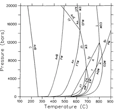
APPLICATION TO THE SYSTEM MgO-SiO2-H2O

In this section, experimental data in the system MgO-SiO2-H2O are used to derive an

optimal set of thermodynamic properties for 10 phases: orthoenstatite (E), talc (T), forsterite (F), quartz (Q), anthophyllite (A), chrysotile (C), antigorite (An), brucite (B), periclase (P), and H2O (W). This system provides an excellent opportunity to apply the

mathe-matical programming techniques discussed above, both because of the wealth of calori-metric and phase equilibrium data, and because the technique can be used to resolve inconsistencies among experimental data, and uncertainties in phase relations which have been controversial.

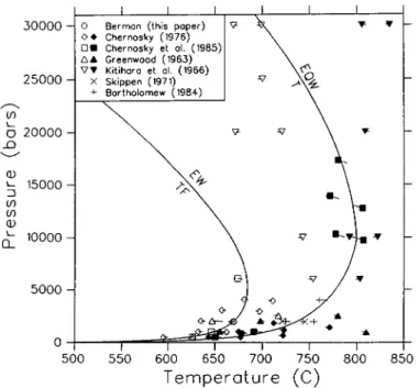
Greenwood (1963) was the first to undertake a systematic study of the stability field of anthophyllite. He studied 6 different equilibria (Table 4), and suggested that the vapor-conservative TEA equilibrium bounds the anthophyllite stability field at approximately 20 kb. On the basis of additional experimental data on two equilibria studied by Greenwood, Chernosky (1976) suggested an upper stability limit of c. 5 kb. Solubility experiments of 8 different assemblages (Hemley et al, 1977a, b) led these authors to propose the existence of two invariant points that bound the anthophyllite stability field only at low pressure.

(16)

Chernosky & Autio (1979) presented additional experimental data for two of the equilibria studied by Greenwood (1963), and were led to favour the topology of latter phase diagram, but they did not rule out the possibility of invariant points limiting the anthophyllite stability field at high pressure. Very recently, Chernosky et al. (1985) presented phase equilibrium data for 5 of the 6 equilibria originally studied by Greenwood, as well as data for the TEA equilibrium. These data, when combined with the large amount of precise calorimetric measurements, place extremely tight constraints on phase relations in this system, with little latitude for further change. We present a thermodynamic analysis of this extremely well studied system in order to illustrate the advantages of the mathematical programming technique in providing a means to (a) resolve inconsistencies between data, and (b) derive an optimal set of thermodynamic properties of phases in this system which are consistent with most available data and which permit phase relationships to be calculated with confidence. The results have important applications to the metamorphism of ultramafic rocks, in so far as denning the stability fields of mineral assemblages in this system.

Calorimetric and volumetric data

Calorimetric and volumetric data listed in Table 3 were used to constrain the thermodynamic properties of phases within the uncertainties of these data. Because enthalpies of formation cannot be determined directly with the accuracy needed for calculating phase relations (see, for example, the range of values reported for forsterite and enstatite in Table 3) only the values of quartz, periclase, and H2O were fixed during the

analysis in order to provide reference enthalpies for each component in the system. Agreement with the calorimetrically determined Af H° for other minerals was sought during

the final optimization discussed below.

Previous LIP studies have not considered uncertainties in reported molar volumes of minerals (e.g., Day & Halbach, 1979; Chatterjee et al, 1984; Day et al, 1985). However, comparison of different determinations of molar volumes for most minerals indicates significant uncertainties, which in many cases are somewhat greater than the precision of individual measurements. Different determinations of the molar volume of talc, for example, do not agree within the quoted uncertainties of the measurements, and probably reflect real differences between samples synthesized under different conditions, and perhaps with different degrees of stacking disorder. We account for the uncertainties in these data by placing bounds on the volume of this phase which span the total range of all precise and apparently accurate determinations. Consequently, the derived thermodynamic properties can be considered to be representative of the 'average' phase used in the calorimetric and phase equilibrium studies. We have constrained the molar volume of anthophyllite within the uncertainty of the data for the synthetic phase studied by Chernosky et al (1985), which are in good agreement with the data for the natural sample measured by Krupka et al (1985b). These data indicate a slightly larger value than reported by Greenwood (1963), and used by Day et al, (1985) in their analysis of this system.

Volumetric data at elevated pressure and temperature are not available for the hydrous phases considered in this study. Because the calculated position of most equilibria (in particular dehydration reactions with large values of Ar H and Ar S) are relatively insensitive

to variations of the volume of minerals at pressures less than 10 kb and temperatures less than 1000 °C (c.f. Helgeson et al, 1978, pp. 30-3), and because estimation of mineral expansivities and compressibilities would introduce an additional and unnecessary source of uncertainty in the calculations, we have assumed that molar volumes of minerals (with the exception of quartz, discussed below) are independent of pressure and temperature.

(17)

T H E R M O D Y N A M I C DATA TABLE 3

Calorimetric and volumetric data for MSH phases

1347 Anthophyllite Antigorite Brucite Chrysotile Orthoenstatite Forsterite Periclase Quartz Talc H2O AyH° (kJ mol ')* - 1 2 0 8 6 0 0 + 7-6 -924-54 + 0-4 -4364-33 ±3-4 -1546-63+ 2 0 t -1548-95+1-3 -1548-38+1-4 -2176-21+ l-3t -2171-56 + 2-2 — 2176-96± 1-5 -2174-25+1-6 -2171-69+1-7 -2172-32+1-8 — 2173-53+ 1-8 -601-50 + 0-30 -910-70 ± 1 0 -5915-90 ±4-3t -285-83 ±0-04 S'{Jmol->) 53700 ±2-7 3598-53 ±26-8 6318 + 013 221-33 + 1-7 66-27 ± 0 1 0 9 4 1 1 + 0 1 0 26-95±015 41-46 ±0-20 260-79 ±0-80 69-95 ± 0 0 8 V° (cm2 mol'1) 265-44 ±0-42 1749-13 ±8-7 24-63 + 0-07 107-46 + 0-42 31-312 + 0-02 43-79 + 0-03 11-25 ± 0 0 1 22-688 ± 0 0 1 136-25 ±0-26 Reference Weeks (1955) Krupka et al. (19856) Chernosky et al. (1985) King et al. (1967) Kunze (1961) Robie et al. (1979)

Giauque & Archibald (1937) Robie et al. (1967) King et al. (1967) King et al. (1967) Chernosky (1975) Brousse et al. (1984) Charlu et al. (1975) Shearer & Kleppa (1973) Krupka et al. (19856) Brousse et al. (1984) Shearer & Kleppa (1973) Brousse et al. (1984) Torgeson & Sahama (1948) Charlu et al. (1975) King et al. (1967) Kiseleva et al. (1979) Kiseleva et al. (1979) Robie et al. (1982) Robie et al. (1967) CODATA (1978) CODATA (1978) Krupka et al. (1979) CODATA (1978) CODATA (1978) Robie et al. (1979) Barany(1963) Robie & Stout (1963) Robie et al. (1967) CODATA (1978) CODATA (1978) * All values computed using heat capacity functions of Berman & Brown (1985).

t Values not used in final optimization for reasons discussed in text.

Heat capacities of minerals are represented by the equation:

w h e r e , for Trcf <T< T;,

(14)

(14a)

Quartz is the only phase considered in this study which undergoes a lambda transition. Equation 14a provides for reasonably accurate representation of its CP to within

approximately 30° of the transition, and equations presented in appendix II of Berman & Brown (1985) allow for calculation of the thermodynamic properties of quartz at elevated pressures. In order to reproduce the PT position of the polymorphic transition (Mirwald & Massonne, 1980) with the assumption that the volume of /?-quartz is constant, it is necessary to consider the volume of a-quartz as a function of P and T (c.f. Helgeson et al., 1978,

(18)

TABLE 4

Phase equilibrium data and associated uncertainties used in mathematical programming analysis

T = 3E Q W A = 7E Q W T F = 5E W 9T 4F = 5A 4W A F = 9E W 7T = 3A 4Q 4W P range (bars) 500-1000 10000-17000 500-1803 2000 2000-4000 1000-2600 6000-30000* 1000-2600 10000 500-3000 2000 2000-2600 500-6000 500-4000 6000-30000* 2000 1000-4000 500-6000 2000-2600 500-6000 500-3000 1000-5000 2000 T range (°C) 656-700 785-800 648-766 726-740 730-770 662-805 800-840 750-772 810 664-775 750 658-712 621-679 600-706 680-750 651-665 663-694 597-716 695-712 632-735 647-742 694-775 715-730 No. 2 5 8 2 3 4 6 5 1 9 1 2 3 10 7 2 7 12 2 9 10 5 2 Apparatus^ CS PC CS CS CS CS PC CS PC CS CS CS CS CS PC CS CS CS CS CS CS CS CS Errors P 1% 300 2% 20 20 50 5% 50 300 20 5% 50 1% 2% 5% 20 50 1% 50 1% 20 50 5% usedX T 6-9 10 5 5 10 5-7 10 5-10 10 5-7 5 5-11 5-6 5 10 5 5 6-10 5 5-9 5-7 5-12 7 Reference Chernosky et al. (1985) Chernosky et al. (1985) Chernosky (1976) Skippen (1971) Bartholomew (1984) Greenwood (1963) Kitahara et al. (1966) Greenwood (1963) Chernosky et al. (1985) Chernosky & Autio (1979) Fyfe(1962)

Greenwood (1963) Chernosky et al. (1985) Chernosky (1976) Kitahara et al. (1966) R. G. Berman (see text) Greenwood (1963) Chernosky et al. (1985) Greenwood (1963) Chernosky et al. (1985) Chernosky & Autio (1979) Greenwood (1963) Fyfe (1962)

o

CO m SO 2

(19)

T 4 E = A 5C = 6F T 9W C B = 2F 3W An = 18F 4T 27W B = P W Q = S C 2S = 2T W An 30S = 16T 15W T = 3E S W 7T = 3A 4S 4W 2A = 7F 9S 2W A = 7E S W 2E = F S T 6 H+ = 3 M g+ + 4S4W 10200-16 700 500-6500 1113 1000-3000 10000-30000* 20000-30000* 500-7000 2000-6000 10000-15000 3950-8230 240-2000 17000-33000* 2000* 1000-2000 250-1000 1-2000* 1000* 1000 1000 1000 1000 1000 1 755-790 399-536 430-440 425-475 560-610 450-540 330-440 480-590 615-660 690-811 554-664 920-1100 665-676 Equilibria 200-500 250 90-450 300-450 649-690 640-670 650-670 660-715 680-720 29815 3 11 2 6 4 5 12 6 4 12 7 6 2 involving 22 6 12 5 5 4 3 10 5 2 PC CS cs cs PC PC cs cs PC IH cs PC cs aqueous silica (S)§ CS CS CS CS CS CS CS CS CS 300 2% 2% 2% 5% 5% 5% 5% 5% 1% 30 5% 5% 50 10 2% 2% 1% 1% 1% 1% 1% 10 6-10 10 10 10 10 10 5 10 5 5 12 3 5 3 5 5 5 5 5 5 5 Chemosky et al. (1985) Chemosky (1982) Kalinin & Zubkov (1981) Scarfe&Wyllie(1967) Kitahara et al. (1966) Kitahara et al. (1966) Johannes (1968) Evans et al. (1976) Evans et al. (1976) Schramke et al. (1982) Barnes & Ernst (1963) Irving et al. (1977) Franz (1982)

Hemley et al. (1980)

Ragnosdottir & Walther (1983) Hemley et al. (1977a)

Hemley et al. (19776) Hemley et al. (19776) Hemley et al. (19776) Hemley et al. (19776) Hemley et al. (19776) Hemley et al. (19776) Bricker et al. (1973) X m 50 o rj w • < Z > o

o

* Data not used in final analysis for reasons discussed in text; see figures for comparison with these data. t Apparatus: CS = cold seal, IH = internally heated, PC = piston-cylinder.

t Tabulated uncertainties were accepted as reported, except that 3° were added to temperature variations reported by Chemosky & Autio (1979),

Chemosky et al. (1985), and Barnes & Ernst (1963) in order to account for estimated calibration uncertainties. § Uncertainties in aqueous silica concentration taken as 5 per cent.

(20)

pp. 81-5). Constant values of (dV/8T)P = 5-4212 x 1(T5 J '1 K "1 and (dV/dP)T = — 2-356 x 1 0 ~6J b ~2 are consistent with these data, the Q. function for quartz (Table 5), and

the transition slope of 0-0237 k b "1.

CP coefficients used in our analysis (Table 5) were taken from Berman & Brown (1985),

with three exceptions. Preliminary MAP analysis showed that several phase equilibrium experiments were inconsistent with the calorimetrically determined entropy of orthoenstatite (Krupka et al., 1985£>) using the CP function for this phase of Berman and Brown (1985). A CP

function consistent with all data (Table 5) was derived in the MAP analysis by the technique described above, and is only very slightly different (within 0-02 per cent) from the function determined from regression of the CP data alone.

The CP of chrysotile given by Berman & Brown (1985) was obtained using their predictive

model, while their CP function for antigorite may be somewhat in error due to uncertainties

introduced by correcting the original CP data to the antigorite formula used in this study.

Both functions were modified (within 2 per cent) during MAP analysis of phase equilibrium data in order to improve agreement with the calorimetrically determined entropy and phase equilibrium constraints.

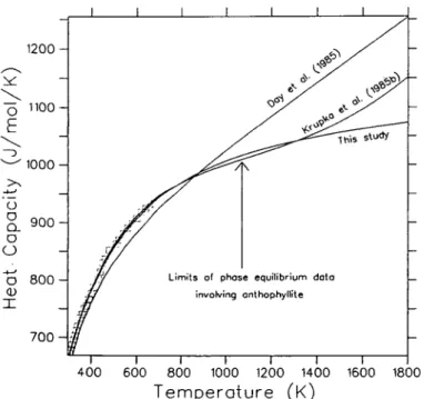
Several additional points are worthy of mention. The calorimetric data for anthophyllite and talc have been measured up to 680 and 640 K, respectively, whereas phase equilibria involving these phases have been studied up to 1070 K. The form of the CP function (14)

allows for reliable extrapolation to high temperature, as discussed by Berman & Brown (1985), and use of this equation can lead to significantly different standard state properties than those derived using the Maier-Kelley equation. The natural sample of Fe-bearing anthophyllite used in the DSC measurements contained approximately 90 per cent of the Mg end-member. The function given in Table 5 was derived by correcting the original data for all impurities using the oxide CP coefficients given by the predictive model of Berman &

Brown (1985).

Analysis of phase equilibrium data

Phase equilibrium data relevant to the MSH system are presented in Table 4. Chernosky (1976) originally pointed out an apparent inconsistency between his data for FT = EW and the data of Greenwood (1963) for FT = AW. The LIP analysis of Day & Halbach (1979) utilized only the data of Chernosky because of unresolved inconsistencies with the data of Greenwood which they suggested were most apparent in the data for A = EQW and T F = EW. Nor did these authors utilize the solubility data of Hemley et al. (1977a, b), or the estimated positions for several univariant equilibria based on these data. Day et al. (1985) recently presented a LIP analysis of this system, but they also considered only the phase equilibrium data of Chernosky and co-workers. Our analysis differs in substance from that of Day et al. (1985) in that all phase equilibrium data are considered and incompatibilities are addressed.

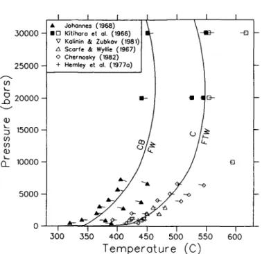
Preliminary analysis of the data in Table 4 indicated major inconsistencies between several sets of data, which we discuss below. The solubility data of Hemley et al. (1977a, b) for chrysotile and antigorite are incompatible with the results of hydrothermal experiments on the equilibria C = FTW (Chernosky, 1982) and An = FTW (Evans et al., 1976). The latter data suggest larger stability fields for both serpentine minerals, a discrepancy that cannot be due solely to the use by Hemley et al. of natural materials with 2-5 wt. per cent impurities. The hydrothermal data were favoured for the following reasons: (a) the higher temperatures of experiments by Chernosky (1982) and Evans et al. (1976) reduces the influence of kinetic factors; their results are internally consistent and show substantial amounts of reaction; and

(21)

TABLE 5

Coefficients for calculation of heat capacity {J mol~l K'1) with equation 14

Mineral Anthophyllite Antigoritet Brucite Chrysotilef Orthoenstatitef Forsterite Quartz a = /?§ Talc Formula Mg7Si8O22(OH)2 Mg48Si34O85(OH)62 Mg(OH)2 Mg3Si2O5(OH)4 MgSiO3 Mg2SiO4 SiO2 Mg3Si4O10(OH)2 1219-31 7394-51 136-84 61002 166-58 238-64 8001 848 664-11 -57-665 0 0 -5-371 -55-812 - 1 2 0 0 6 - 2 0 0 1 3 -2-403 499 -51-872 fc2x/0"3 -347-661 -5483-630 -43-619 -18-573 -22-706 0 0 -35-467 -009187 -21-472 k3x / 0 -7 440090 8728-412 55-269 19-547 • 27-915 -11-624 49157 00002461 -32-737 Range (K) 250-385 344-679 276-296 405-847 253-299 350-666 256-296 400-1000 254-385 344-999 973-1273 253-299 304-380 398-1807 250-290 400-820 373-1373 1001-1676 250-290 349-639 A AD* 007 0-46 0-82 0-99 0-32 014 007 0-52 006 0-37 0-84 0-08 0-89 0-21 019 0-32 0-57 0-81 0-62 0-23 Reference Krupka et al. (1985b) Krupka et al. (1985a) King et al. (1967)} King et al. (1967)}

Giauque & Archibald (1937) Kinget al. (1975)

King et al. (1967)

Estimated (Berman & Brown, 1985) Krupka et al. (1985b)

Krupka et al. (1985a) Haselton (1979) Robie et al. (1982) Robie et al. (1982) Orr (1953)

Westrum (unpublished data) Ghiorso et al. (1979) White (1919) Richet et al. (1982) Robie & Stout (1963) Krupka el al. (1985a)

H X m

o

a

• <

z

—

o D H

* Average absolute per cent deviation of data from adopted function. t CP function adjusted by analysis of phase equilibrium data (see text).

% Data adjusted to molecular weight of antigorite used in this study.

§ Tabulated values: transition temperature, 7)(K), heat of transition (J moP1), (i in (J moP1)0'5/K, and l2 in (J mol~')°'5/K2 of equation 14a; Trcf = 373 K

(22)

(b) Chernosky's (1982) data are for the most part consistent with all other chrysotile equilibria listed in Table 3, and with the data of Johannes (1969) for equilibria involving mixed volatiles (Berman et al, 1985).

Thermodynamic properties of chrysotile and antigorite derived from the solubility data of Hemley et al. (1977a, b) lead to the metastability of chrysotile above 298-15 K (e.g., Helgeson

et al, 1978). Although kinetic factors (e.g., Dungan, 1977) and solid solution effects

complicate interpretation of natural occurrences, the widespread occurrence of chrysotile in low T serpentinites (e.g., Evans et al, 1976; Evans, 1977) suggests a true stability field for this phase. Consequently, we have added a 'field' constraint to the problem which consists of a low-temperature 'half-bracket' for the C = AnB equilibrium at 250 °C and 2 kb. This temperature represents the maximum temperature for this equilibrium that allows con-sistency with other phase equilibrium and calorimetric data (Tables 3 and 4). This kind of 'artificial' data point is extremely useful for imposing constraints from natural occurrences, and is similar in intent to the parametric programming procedures discussed by Halbach & Chatterjee (1982).

MAP analysis of all phase equilibrium data involving the phases F, T, A, E, and W prior to publication of the data of Chernosky et al. (1985) revealed a major inconsistency in these data: all data in Table 4 are mutually consistent with either Chernosky's (1976) data for FT = EW or Greenwood's (1963) data for FT = AW, but not with both. As details of experimental procedures reported in both studies did not reveal the source of the disagreement, resolution of this inconsistency required additional experiments, and it seems worthwhile to note that the design of key experiments is a major advantage of the mathematical programming approach. Experiments performed at UBC in the past year using synthetic materials provide a 2 kb bracket for the FT = EW equilibrium (Table 4), which corroborates the results of Chernosky (1976). Chernosky et al (1985) recently reported data for FT = AW that indicates equilibrium approximately 20° below the position determined by Greenwood (1963). In an attempt to discover the source of this discrepancy, we have reexamined Greenwood's unpublished experimental run notes, and found that critical FTAW runs used starting materials that included small amounts of cristobalite and enstatite, in addition to the phases involved in this equilibrium. It now seems likely that changes in the amount of anthophyllite observed in some experimental runs by Greenwood (1963) were due to the operation of reactions other than the FTAW reaction.

In light of this discussion, we have used in our MAP analysis all available phase equilibrium data (Table 4), except for those experiments that involved extraneous phases either in starting materials (Greenwood, 1963) or in run products (Chernosky, 1976, 1982; Chernosky et al., 1985), and in which the observed changes in the proportions of reactants and products were contradictory (e.g., TE = A experiments of Chernosky et al., 1985). In addition, we did not use any data above 15 kb due to uncertainties in the thermodynamic properties of H2O at high pressures, and because mineral compressibilities/expansivities

were not included in our equations of state. All phase equilibrium data were adjusted for reported or estimated uncertainties (precision and accuracy) in pressure, temperature, and composition (Table 4) as described above.

Results

The final solution of the MAP problem was obtained using the objective function (relation 12) which minimizes discrepancies with calorimetric and volumetric measurements. All data shown in Table 3 were used in the final optimization except for Af//° values of talc

(23)

PHASES

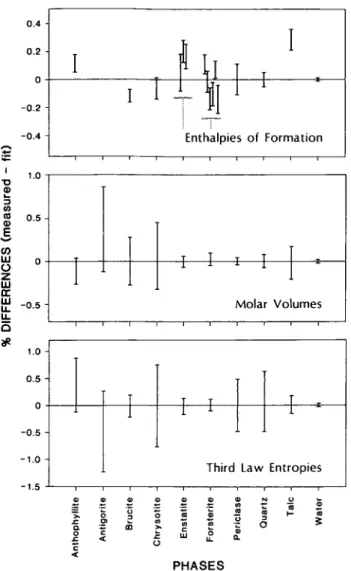
FIG. 4. Comparison of thermodynamic properties derived by MAP analysis of all experimental data (zero base line) with direct measurements on phase properties. All derived properties are consistent within the uncertainties of the

measurements except for the Af H° values for talc, anthophyllite, and brucite (see discussion in text).

latter two values were excluded because the range of reported values precluded selection of 'best' values.

The thermodynamic properties of phases in this system which result from our analysis are listed in Table 6, and shown in comparison to calorimetric values in Fig. 4. For volumes and third law entropies, all fit values lie within the uncertainties of measurements, a result that is particularly satisfying given the diverse nature of the phase equilibrium data utilized in this analysis, and the extremely small uncertainties associated with the recent calorimetric measurements of Krupka et al. (1985b). Although the analysis of phase equilibrium data in this system led Day et al. (1985) to the conclusion that the calorimetrically determined entropy of anthophyllite might be in error, our analysis indicates that the phase equilibrium and calorimetric data are in good agreement. The different results of Day et al. (1985) appear to be related, at least in part, to the procedure they used to correct the Cp data for a natural anthophyllite to its end-member composition. The Cp function adopted by Day et al. is