The environmental dependence of the structure of outer galactic discs in STAGES spiral galaxies
18
0
0
Texte intégral
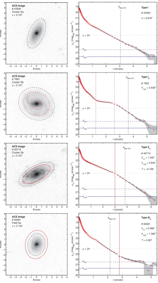
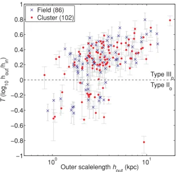
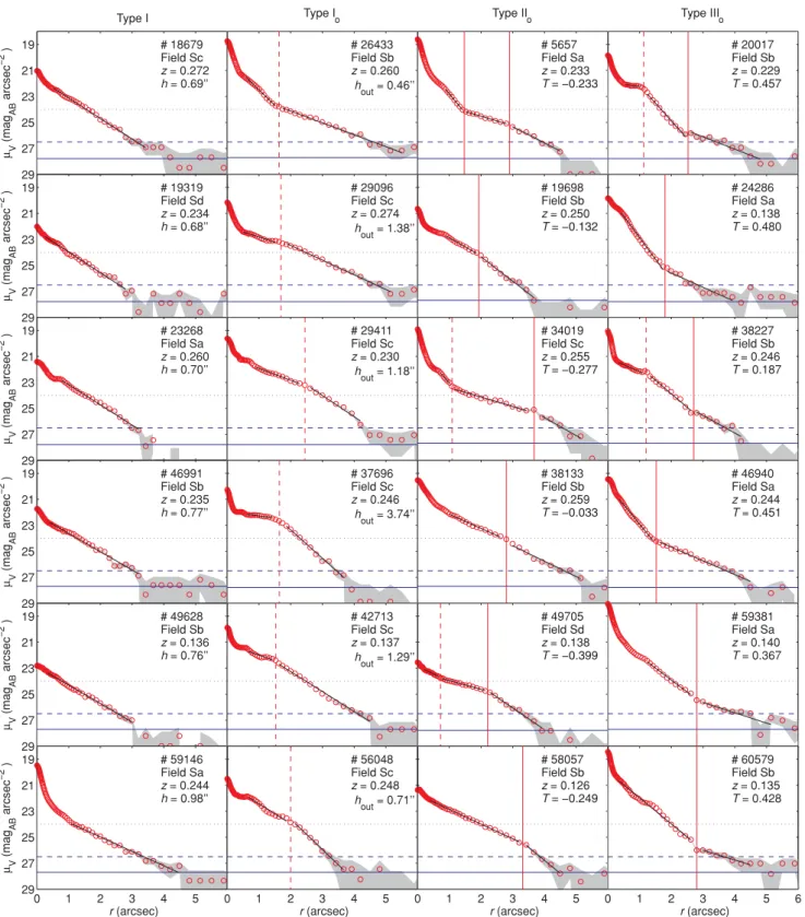
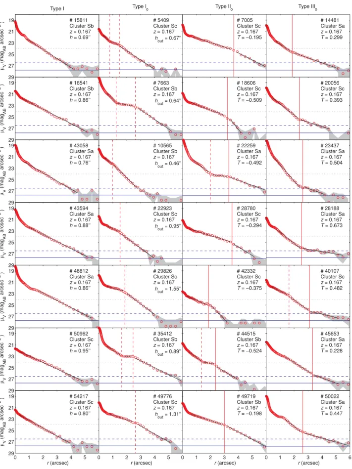
Figure
+7
Documents relatifs
