Common problematic aspects of coupling hydrological models with groundwater flow models on the river catchment scale

HAL Id: hal-00296957

https://hal.archives-ouvertes.fr/hal-00296957

Submitted on 26 Sep 2006

HAL is a multi-disciplinary open access

archive for the deposit and dissemination of

sci-entific research documents, whether they are

pub-lished or not. The documents may come from

teaching and research institutions in France or

abroad, or from public or private research centers.

L’archive ouverte pluridisciplinaire HAL, est

destinée au dépôt et à la diffusion de documents

scientifiques de niveau recherche, publiés ou non,

émanant des établissements d’enseignement et de

recherche français ou étrangers, des laboratoires

publics ou privés.

Common problematic aspects of coupling hydrological

models with groundwater flow models on the river

catchment scale

R. Barthel

To cite this version:

R. Barthel. Common problematic aspects of coupling hydrological models with groundwater flow

models on the river catchment scale. Advances in Geosciences, European Geosciences Union, 2006, 9,

pp.63-71. �hal-00296957�

www.adv-geosci.net/9/63/2006/

© Author(s) 2006. This work is licensed under a Creative Commons License.

Advances in

Geosciences

Common problematic aspects of coupling hydrological models with

groundwater flow models on the river catchment scale

R. Barthel

Institute for Hydraulic Engineering, Universitaet Stuttgart, Germany

Received: 23 January 2006 – Revised: 22 May 2006 – Accepted: 3 July 2006 – Published: 26 September 2006

Abstract. Model coupling requires a thorough conceptuali-sation of the coupling strategy, including an exact definition of the individual model domains, the “transboundary” pro-cesses and the exchange parameters. It is shown here that in the case of coupling groundwater flow and hydrological models – in particular on the regional scale – it is very impor-tant to find a common definition and scale-appropriate pro-cess description of groundwater recharge and baseflow (or “groundwater runoff/discharge”) in order to achieve a mean-ingful representation of the processes that link the unsatu-rated and satuunsatu-rated zones and the river network. As such, integration by means of coupling established disciplinary models is problematic given that in such models, processes are defined from a purpose-oriented, disciplinary perspec-tive and are therefore not necessarily consistent with defi-nitions of the same process in the model concepts of other disciplines. This article contains a general introduction to the requirements and challenges of model coupling in Inte-grated Water Resources Management including a definition of the most relevant technical terms, a short description of the commonly used approach of model coupling and finally a detailed consideration of the role of groundwater recharge and baseflow in coupling groundwater models with hydro-logical models. The conclusions summarize the most rele-vant problems rather than giving practical solutions. This paper aims to point out that working on a large scale in an integrated context requires rethinking traditional disciplinary workflows and encouraging communication between the dif-ferent disciplines involved. It is worth noting that the aspects discussed here are mainly viewed from a groundwater per-spective, which reflects the author’s background.

Correspondence to: R. Barthel (roland.barthel@iws.uni-stuttgart.de)

1 Introduction

Model coupling (or rather, model concepts) on a large or regional scale (∼104–105km2)is a common task in mod-ern integrated water resources management (IWRM). It has become apparent – in particular in Global Change research – that processes must inevitably be perceived in an inte-grated way. The impacts of climate change can not be eval-uated meaningfully without considering, for example, land use changes (subsequent or independent) or other natural and socio-economic developments. As fully integrated holis-tic model concepts (i.e. models which do not just comprise several individual “old” models) for this purpose do not ex-ist (yet), one means of integration is the coupling of exex-ist- exist-ing disciplinary models. Problems arise here because disci-plinary models were usually originally designed to solve spe-cific problems in different domains of the water cycle. The processes and the process descriptions they include and the extent of their domain of interest was adapted to a typical class of problems. Therefore the coupling of two or more disciplinary models is associated with conceptual inconsis-tencies and incompatibilities because the individual models may describe the same process differently, may ignore im-portant connecting processes or overlaps and gaps between the model domains may exist. This paper cannot cover the field of model coupling in hydrology extensively. A broad overview is given by Bronstert et al. (2005).

GLOWA-Danube (http://www.glowa.org) and Rivertwin (http://www.rivertwin.org) are interdisciplinary, interna-tional projects that attempt to develop integrated strategies and tools for water and land use management. Within these projects the author’s research group is responsible for the groundwater domain and its connections to the other do-mains of the hydrological cycle as well as to human ac-tivities. After approximately five years of intensive de-velopment of strategies to couple groundwater models to SVAT (soil-vegetation-atmosphere-transfer) and hydraulic

64 R. Barthel: Common problematic aspects of coupling hydrological models

and hydrological models on the very large scale (catch-ments of 80 000 and 14 000 km2, respectively the Danube and Neckar), it has become apparent that the concept of inter-disciplinary model coupling requires a new outlook on cer-tain aspects of the hydrological cycle.

It is shown here that it is crucial to include several con-siderations in the coupling strategy to achieve any valuable coupling of hydrological and groundwater models; it must be ensured that processes, parameters, model discretisation (spatial and temporal) are defined coherently on either side. Neither gaps nor overlaps of model domains and processes may exist. The scale and context dependency of models must be considered, in particularly with regard to the anticipated applications of the coupled (or integrated) model. In this pa-per, two terms that are usually of great importance in the at-tempt to relate surface and subsurface processes were chosen to demonstrate the importance of the aforementioned con-siderations: groundwater recharge and baseflow (or ground-water runoff/discharge; from here on regarded as synonyms even though distinctions would be possible). These appar-ently well-known, well-defined terms are, if analysed in de-tail, highly dependent on scale and context. Moreover they are understood differently in “surface” and “subsurface hy-drology” (groundwater, saturated flow, hydrogeology etc.) depending on the main focus of interest (saturated – unsatu-rated flow processes etc.). As will be shown later, it is of sig-nificance whether we look at groundwater recharge mainly as something getting into the saturated zone or as something leaving the unsaturated zone. A detailed analysis of this as-pect reveals a “forgotten domain” of the hydrological cycle that has neither gained much interest from groundwater nor unsaturated zone researchers: the deeper unsaturated zone, located between the bottom of the root zone and the ground-water level (or aquifer top in case of a confined situation), see Harter and Hopmans (2004) for a detailed discussion.

Before starting a detailed description of the problem, some terms – as they are used in the context of this paper – will be defined. A catchment refers to river catchments in the range of 103to 105km2and more. This scale is referred to as “re-gional”. A system means a main component or domain of the hydrological cycle (compartment); e.g. the “groundwa-ter system”, or the “unsaturated zone (system)”’. The “groundwa-term model includes both the actual model, as one representation of a real natural system, as well as the “model concept” (a mathematical or verbal formulation of processes without ref-erence to a certain location). In this paper, Groundwater models are flow models that simulate piezometric heads, flow directions and fluxes in one or more aquifers, discretized in grids or elements according to the actual geometry of geo-logical layers. Groundwater models as introduced here are limited to simulation of saturated zone processes. Hydro-logical models are less specifically defined as models that simulate the water cycle of a catchment with a focus on pro-cesses near the land surface, including soil and the unsat-urated zone but not describing the groundwater system

ex-plicitly. This definition may include everything from simple black box models to highly parameterized physically based models. Finally, parameter refer to (dimensionless) calibra-tion parameters, whereas variables define measurable quan-tities (physical parameters). The author is aware of the fact that using the terms “parameter” and “variable” in this way might be misleading, since they are used differently by differ-ent disciplines. According to the author’s experiences from interdisciplinary projects, it is crucial to define these seem-ingly “common sense terms” in order to avoid severe misun-derstandings and subsequently bad model results.

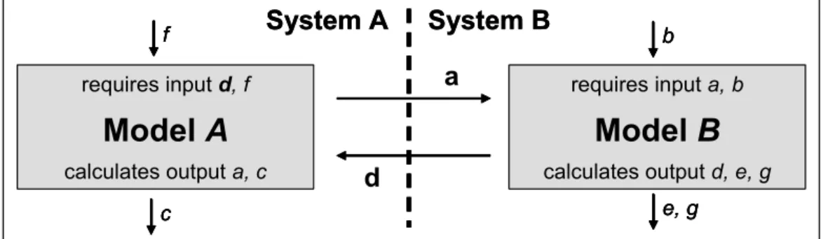
Finally the term model coupling itself has to be defined: Model coupling here means coupling of distinct existing models or model concepts that were developed to simulate processes in one “system”, e.g. coupling of a typical model concept for the saturated zone (MODFLOW; McDonald and Harbaugh, 1988) with a typical hydrological model concept (HBV; Bergstr¨om, 1995). Coupling in the present context mainly means coupling via exchange variables rather than directly coupling process equations and code (see Fig. 1).

2 Model coupling on the large scale

Coupling of models on the regional scale is relatively new and no generalised concepts exist. The problems and is-sues are manifold, in particular since each catchment and each problem has its special characteristics and requirements. Therefore a detailed consideration is not possible here. It is however necessary to at least mention the most important is-sues in order to make clear, that those aspects dealt with in more detail later are only two out of many. Considerations related to model coupling on the large scale can be classified in three main categories:

1. Aspects related to modelling on the large scale in gen-eral

2. Aspects related to model coupling in general

3. Specific aspects related to model coupling on the large scale

Aspects of the first category are: data requirements and data availability, discretisation and scaling aspects (pro-cesses, variables and parameters) and computational de-mands. It is worth mentioning here that even if the model is quite fast a thorough analysis of the huge amounts of model result data beyond looking at performance criteria can be very time consuming. Since these problems are well known and not very specific, they will not be dealt with from here on.

The second group of aspects is related to coupling of sys-tems that are governed by different processes and variables (and consequently equations) and that have different focal points on spatial and temporal scales. A lot of research has

R. Barthel: Common problematic aspects of coupling hydrological models 65

Bronstert et al., 2005). Again, no further discussion is made here.

Finally the third group combines the problems acknowledged from the first two groups and adds

new ones. In the author’s opinion, the most eminent issue in coupling models on a large scale

(third category aspects) seems to be the need for a real joint model calibration. Joint calibration in

general should be beneficial (at least theoretically) because it allows calibration against more than

one output variable (e.g. Seibert, 2000). This advantage however decreases quite rapidly as the

model area increases due to the computational capacity required. Large scale groundwater flow

models are usually quite slow. As a consequence, automatic, iterative calibration and

optimisation procedures can not usually be applied successfully.

3

Development of coupling strategies

Within the scope of this paper, it is assumed that the basic coupling strategy is as shown in Figure

1. Model A, which represents system A, calculates an output which forms an input for model B

(system B). It is furthermore assumed that the coupling strategy is mainly based on the use of

existing model concepts rather than on the development of new ones. For the remaining part of

this paper Model A is a hydrological model, Model B represents a groundwater flow model.

requires input a, b

Model B

Model A

a

d

System A

System B

Model B

Model A

a

d

System A

System B

Figure 1: Coupling two models using exchange variables, where some of the output variables of one model form

input variables for the other. a and d are exchange variables used for coupling.

The first step in attempting to couple two models that describe different but interdependent

systems should be the consideration of some basic questions. They include the questions that

should generally be asked before starting to model. These questions relate to the problems the

coupled model complex will be used to solve, the output variables that are required, the relevant

5

Fig. 1. Coupling two models using exchange variables, where some of the output variables of one model form input variables for the other.

aand d are exchange variables used for coupling.

been dedicated to these aspects (see e.g. Bronstert et al., 2005). Again, no further discussion is made here.

Finally the third group combines the problems acknowl-edged from the first two groups and adds new ones. In the author’s opinion, the most eminent issue in coupling mod-els on a large scale (third category aspects) seems to be the need for a real joint model calibration. Joint calibration in general should be beneficial (at least theoretically) because it allows calibration against more than one output variable (e.g. Seibert, 2000). This advantage however decreases quite rapidly as the model area increases due to the computational capacity required. Large scale groundwater flow models are usually quite slow. As a consequence, automatic, iterative calibration and optimisation procedures can not usually be applied successfully.

3 Development of coupling strategies

Within the scope of this paper, it is assumed that the basic coupling strategy is as shown in Fig. 1. Model A, which represents system A, calculates an output which forms an in-put for model B (system B). It is furthermore assumed that the coupling strategy is mainly based on the use of existing model concepts rather than on the development of new ones. For the remaining part of this paper Model A is a hydrologi-cal model, Model B represents a groundwater flow model.

The first step in attempting to couple two models that de-scribe different but interdependent systems should be the consideration of some basic questions. They include the questions that should generally be asked before starting to model. These questions relate to the problems the coupled model complex will be used to solve, the output variables that are required, the relevant scales, the required accuracy of the results, the data availability etc. As considering these general question should be a standard procedure in model conceptualisation, the topic is not elaborated on.

In addition to these general issues there are a number of questions that relate specifically to model coupling of two systems:

– How are the individual systems defined and what are the (dominant) processes that take place in each system? – Where and what is the boundary between the systems?

Is it a sharp and stable or just a virtual, time-dependent boundary?

– Which processes connect the systems to each other? Are the connecting processes clearly related to pro-cesses that take place within the individual systems? – Which process descriptions are needed, which are

avail-able, which are applicable in view of discretisation and data availability?

– What are the dynamic relations between the two sys-tems (one or bi-directional, feedback, different dynam-ics)?

– Which measurable quantities are available to determine the effect of changes in inputs to the individual system and how do these quantities relate to the connecting pro-cesses?

– What are the relevant process scales (time and space) and how are they related to the scale of the problem? Are the relevant scales equal on either side?

Answers to the questions listed above should lead to the defi-nition of system boundaries, connecting processes, exchange variables and appropriate scales and finally to a first concep-tual description of at least one possible coupling approach.

Once such a conceptualization has been achieved, the next step is to choose (or to develop) the appropriate individual models for each system: “Appropriate” means that the mod-els treat their domain in a way that satisfies the answers to the questions listed above. Whereas internal processes are of minor importance here, the exchange processes and vari-ables require special attention. From Fig. 1 it is clear that an input variable d of model A must be equal to the out-put variable d of model B. In this case, equal means not

66 R. Barthel: Common problematic aspects of coupling hydrological models Atmosphere Biosphere / Landsurface Groundwater Soil / Unsaturated Zone

“Systems”

“Processes”

Output: Groundwater Level / Head Changes

Hydrological ‘Block’

Groundwater Model

Groundwater Recharge

Baseflow

Discharge

System and Process

Simplification

“Systems”

“Processes”

Output: Groundwater Level / Head Changes

Hydrological ‘Block’ Groundwater Model Groundwater Recharge Baseflow Discharge Discharge

System and Process

Simplification

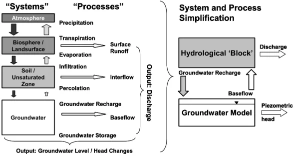
Figure 2: Fundamental systems and processes that are typically considered when groundwater and surface water / unsaturated zone systems are coupled.

4 Groundwater Recharge and Baseflow - Definition and characteristics

As shown in the previous section, groundwater recharge and baseflow are two main processes that link the unsaturated and saturated zones or, in a more specific sense, the link between hydrological and groundwater models. Using the balance terms controlled by these two processes along with interflow and surface runoff, it is seemingly possible to close the hydrological balance of a catchment. Of course storage in the different compartments of the system (groundwater, soil and delayed discharge in the surface and river runoff) also has to be considered.

It is well known that neither groundwater recharge nor baseflow can be measured directly because it is largely unknown where and how these processes take place and because these processes are inaccessible for measuring procedures or cannot be clearly separated from others. Less well known is the fact that no common definition that would be meaningful in the context of large scale models exists for either of these terms. Proof of this is the existence of a large number of methods to determine groundwater recharge as well as baseflow. The methods are conceptually very different and accordingly yield very different results. Groundwater recharge can be directly calculated using physically based approaches (unsaturated flow equations, tracers,

8

Fig. 2. Fundamental systems and processes that are typically considered when groundwater and surface water/unsaturated zone systems are coupled.

only equal units and equal spatial and temporal discretisa-tion – in most cases it will not be too problematic to adjust these values formally by means of conversion, aggregation and dis-aggregation. What is far more important and at the same more difficult to achieve is guaranteeing equality of the exchange variable with respect to “meaning”. Does d calcu-lated by model B really have the same meaning as d required by A? Is it conceptually the same thing?

In the case of coupling hydrological and groundwater models, the first step in developing the coupling strategy, i.e. the identification of systems and connecting processes is con-ceptually quite difficult if all possible processes on all scales are to be considered. In the context of this paper however certain simplifications are made: Firstly it is assumed that the effects of direct evaporation from groundwater, capillary rise, and root water uptake from groundwater (all flows out of the groundwater upwards) can be neglected. We also will assume that fluxes from the ‘surface water’ system (rivers) to the groundwater system are small compared to fluxes in the opposite direction. This allows us to ignore certain compli-cated, non-linear and interdependent feedback processes.

Given these assumptions, the hydrological cycle can be simplified to the situation shown on the right hand side of Fig. 2: a system reduced to a hydrological block (model) and a groundwater block (model) which is consistent with the scheme shown in Fig. 1. The two connecting processes are groundwater recharge, as the quantity leaving the unsatu-rated part and entering the groundwater system, and baseflow as the part leaving the groundwater and entering the surface water system. When all the assumptions and generalisations mentioned above are considered, an apparently simple and straight forward coupling principle can be established.

How-ever, if we have a closer look at this simple scheme we will find that is conceptually problematic because of the weak definitions of the terms it is founded on.

4 Groundwater recharge and baseflow – definition and characteristics

As shown in the previous section, groundwater recharge and baseflow are two main processes that link the unsaturated and saturated zones or, in a more specific sense, the link between hydrological and groundwater models. Using the balance terms controlled by these two processes along with interflow and surface runoff, it is seemingly possible to close the hy-drological balance of a catchment. Of course storage in the different compartments of the system (groundwater, soil and delayed discharge in the surface and river runoff) also has to be considered.

It is well known that neither groundwater recharge nor baseflow can be measured directly because it is largely un-known where and how these processes take place and be-cause these processes are inaccessible for measuring proce-dures or cannot be clearly separated from others. Less well known is the fact that no common definition that would be meaningful in the context of large scale models exists for ei-ther of these terms. Proof of this is the existence of a large number of methods to determine groundwater recharge as well as baseflow. The methods are conceptually very dif-ferent and accordingly yield very difdif-ferent results. Ground-water recharge can be directly calculated using physically based approaches (unsaturated flow equations, tracers, chem-istry, isotopes . . . ) or indirectly using conceptual models

saturated zone -groundwater zone unsaturated zone Precipitation

Groundwater Recharge Type 2:

Standard definition used in groundwater modelling

Infiltration Percolation

Groundwater Recharge Type 1: Definition

used in many physically based unsaturated zone models (also: lysimeters)

Soil or root zone

?

Groundwater Recharge Type 2:

Standard definition used in groundwater modelling

Infiltration Percolation

Groundwater Recharge Type 1: Definition

used in many physically based unsaturated zone models (also: lysimeters)

Soil or root zone

?

?

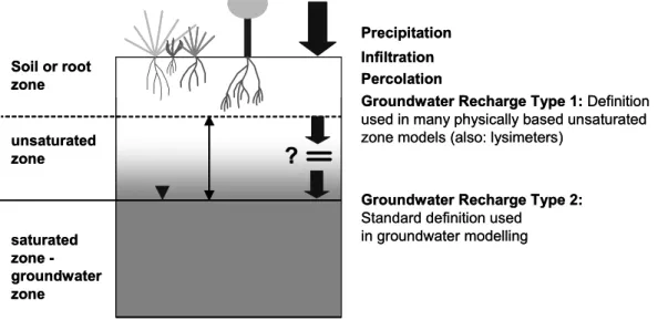
Figure 3: Groundwater recharge - two contrary conceptual interpretations. Type 1: water leaving the root zone, Type 2: water entering the saturated zone.

According to Figure 3, it would be valid to assume that groundwater recharge defined as ‘root

zone percolation’ and groundwater recharge defined as ‘water entering the saturated zone’

describe the same quantities volumetrically. This is only true if volumes are averaged over a

longer period of time, since depending on the distance between the root zone bottom and the

groundwater surface, a temporal delay occurs.

Figure 3 shows a very specific situation with a shallow groundwater table (thickness of root zone

and the total thickness of the unsaturated zone are of the same order of magnitude), a completely

flat relief and homogenous, isotropic conditions. On a larger scale it is highly unlikely that

conditions like this are realized everywhere in a catchment. On a large scale, relief will be present

and the subsurface will usually show heterogeneity. Under such conditions, the scheme shown in

Figure 3 must be replaced with the scheme shown in Figure 4.

10

Fig. 3. Groundwater recharge – two contrary conceptual interpretations. Type 1: water leaving the root zone, Type 2: water entering the saturated zone.

(for an overview of state-of-the-art methods see: de Vries et al., 2002). Baseflow is usually determined using con-ceptual approaches (hydrograph separation, e.g. Tallaksen, 1995) in rare cases also using hydrochemical and isotopi-cal methods but is also isotopi-calculated, using groundwater mod-els, as the amount of water flowing towards a river boundary condition. There is a lot of evidence coming from different studies worldwide that the results of most approaches used to determine the groundwater contribution to river discharge are highly unreliable or at least only valid under very spe-cific conditions for spespe-cific catchments (see e.g. Halford and Mayer, 2000; Vogel and Kroll, 1995).

One reason why so many different methods were estab-lished is the actuality of contrasting catchment characteris-tics and different data availability as well as different scales of application. At the same time, diverse approaches are the result of a different understanding of what recharge and baseflow really are. Conflicting view points across different disciplines can be recognized. In the case of groundwater recharge, two extreme interpretations can be identified:

Groundwater recharge is usually defined as the sum of all inflows to a groundwater system or aquifer. From the groundwater standpoint, this includes all inflows from above, from below and lateral inflows. Only under very specific con-ditions it is possible to measure or calculate all these recharge terms. Therefore even groundwater experts almost always re-duce the recharge definition in practice to the inflows coming from above (precipitation, effluent rivers). But still their fo-cus is usually on the volume of water entering a (specific) aquifer. On the other hand, surface hydrologists and soil scientists usually suppose groundwater recharge to be the amount of water leaving the soil or root zone, since this is the domain they predominantly deal with (see Scanlon et al.,

2002). The basic assumption here is: When water leaves the domain influenced by vegetation (roots) and evaporation (capillary rise etc.) vertically downwards, it will reach the groundwater eventually and must therefore be equivalent to groundwater recharge. Figure 3 exemplifies these two con-tradictory views:

According to Fig. 3, it would be valid to assume that groundwater recharge defined as “root zone percolation” and groundwater recharge defined as “water entering the satu-rated zone” describe the same quantities volumetrically. This is only true if volumes are averaged over a longer period of time, since depending on the distance between the root zone bottom and the groundwater surface, a temporal delay oc-curs.

Figure 3 shows a very specific situation with a shallow groundwater table (thickness of root zone and the total thick-ness of the unsaturated zone are of the same order of mag-nitude), a completely flat relief and homogenous, isotropic conditions. On a larger scale it is highly unlikely that condi-tions like this are realized everywhere in a catchment. On a large scale, relief will be present and the subsurface will usu-ally show heterogeneity. Under such conditions, the scheme shown in Fig. 3 must be replaced with the scheme shown in Fig. 4.

Figure 4 shows a still idealized, simple situation but is more realistic with respect to formation of groundwater recharge. It becomes obvious that in an area with relief, the depth to the groundwater is a relevant factor for any transient model (Fig. 4, left side). Of even greater influence however are heterogeneities such as impermeable or less permeable layers that occur in the unsaturated part between root zone and groundwater (Fig. 4, right side). Such layers of lower permeability can be found everywhere and the deeper the

68 R. Barthel: Common problematic aspects of coupling hydrological models

homogeneous, isotropic groundwater system, same horizontal extend as surface catchment

Assumption: precipitation and infiltration: homogeneously all over the area

isotropic homogeneous

soil – root zone

deep unsaturated zone

river ‘surface runoff’ ‘interflow’ ‘baseflow’ Δh1 Δh2

impermeable / leaky layer spring

root zone percolation = SVAT-groundwater recharge

recharge to the groundwater system recharge

groundwater table

homogeneous, isotropic groundwater system, same horizontal extend as surface catchment

Assumption: precipitation and infiltration: homogeneously all over the area

isotropic homogeneous

soil – root zone

deep unsaturated zone

river ‘surface runoff’ ‘interflow’ ‘baseflow’ Δh1 Δh2

impermeable / leaky layer spring

root zone percolation = SVAT-groundwater recharge

recharge to the groundwater system recharge

groundwater table

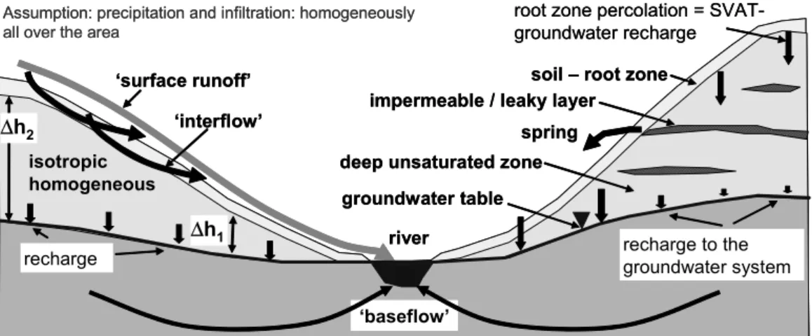
Figure 4: More realistic (compared to Figure 3) but still highly conceptual view of land surface, soil and groundwater processes.

Figure 4 shows a still idealized, simple situation but is more realistic with respect to formation of groundwater recharge. It becomes obvious that in an area with relief, the depth to the groundwater is a relevant factor for any transient model (Figure 4, left side). Of even greater influence however are heterogeneities such as impermeable or less permeable layers that occur in the unsaturated part between root zone and groundwater (Figure 4, right side). Such layers of lower permeability can be found everywhere and the deeper the depth to the groundwater is, the more frequent and the more effective they usually are. They lead to the formation of saturated lenses (perched water) and subsequently to horizontal flow in the deeper unsaturated or partly saturated zone. Flow can be towards neighbouring catchments or can lead to the formation of springs. In either case, the flow does not reach the groundwater system and must therefore not be considered as groundwater recharge.

At this point, a definite gap in the two groundwater recharge definitions in Figure 3 becomes apparent: If less permeable layers are present - or anisotropic, heterogeneous conditions in general -, the recharge actually reaching the groundwater system must be smaller than the recharge leaving the soil / root zone. The horizontal flow induced by the structures in the deep unsaturated zones can cause an overall loss of water from the catchment under investigation or

11

Fig. 4. More realistic (compared to Fig. 3) but still highly conceptual view of land surface, soil and groundwater processes.

depth to the groundwater is, the more frequent and the more effective they usually are. They lead to the formation of sat-urated lenses (perched water) and subsequently to horizontal flow in the deeper unsaturated or partly saturated zone. Flow can be towards neighbouring catchments or can lead to the formation of springs. In either case, the flow does not reach the groundwater system and must therefore not be considered as groundwater recharge.

At this point, a definite gap in the two groundwater recharge definitions in Fig. 3 becomes apparent: If less per-meable layers are present – or anisotropic, heterogeneous conditions in general, the recharge actually reaching the groundwater system must be smaller than the recharge leav-ing the soil/root zone. The horizontal flow induced by the structures in the deep unsaturated zones can cause an over-all loss of water from the catchment under investigation or becomes interflow (i.e., it reaches the surface water system without having been part of the groundwater system after a passage through the unsaturated zone).

The key to this problem would be a better understand-ing or at least a thorough recognition of the conditions and the processes within the deeper unsaturated zone, which was previously named here a “forgotten domain” in hydrological sciences (Harter and Hopmans, 2004). This zone, located between the bottom of the “root zone” and the groundwater level (or aquifer top in the case of a confined situation) can be of considerable thickness on the regional scale (relevant in the range of 10 to 1000 m) and can lead to a difference of up to 100% between root zone percolation and actual recharge to a regional aquifer (see e.g. Rauert et al., 1993; Andres and Egger, 1985). In practical groundwater modelling this is a well known fact (see e.g. Sanford, 2002), however the ap-proaches to deal with this problem (transfer functions) are usually of highly pragmatic rather than of scientific nature (see e.g. Lemmel¨a and Tattari, 1998; Tankersley et al., 1993).

In the previous section it was concluded, that on the large scale at least a part of the water that percolated through the root zone becomes “interflow” after it has been forced to flow horizontally due to less permeable structures (see Fig. 4). In the course of this conclusion, a second problematic aspect becomes apparent; the question of when a saturated domain should be considered as “groundwater” and subsequently when a flow in a saturated domain should be named ground-water flow (baseflow [?]) or better interflow? In the case of Fig. 4 on right hand side, infiltrating water seeps through the unsaturated zone until it reaches an impermeable layer. Here it accumulates and forms a (small [?→scale!]) saturated lens. Depending on the hydraulic conditions within this lens even-tually saturated flow (groundwater flow [?]) will be estab-lished. Whether such a perched (small) saturated lens is con-sidered to be groundwater or if it should be called a (small) saturated domain in a predominantly unsaturated zone now depends on the situation, i.e. the scale and the context. This also determines whether the resulting flow is called “inter-flow” or “groundwater “inter-flow” (baseflow).

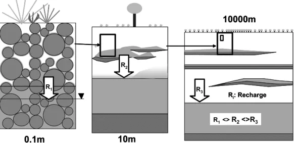
The definition of groundwater, in particular in a modelling context is a highly scale-dependent one. Obviously not any perched or local aquifer or small saturated domain of some m3can be taken into account as groundwater in a regional groundwater flow model, even if the processes within this saturated domain are dominantly saturated flow processes. Figure 5 demonstrates how a clear definition of groundwater as a saturated domain becomes questionable when the rele-vant scale changes over several orders of magnitude. It also shows how a seemingly clearly defined term such as ground-water recharge becomes ambiguous when regarded on dif-ferent scales and in difdif-ferent contexts – depending on which aquifer is relevant for the specific problem. Finally it shows that recharge is not only a question of volume but also of time. Even if the recharge averaged over long periods might

R. Barthel: Common problematic aspects of coupling hydrological models 69

shows that recharge is not only a question of volume but also of time. Even if the recharge

averaged over long periods might be the same, its temporal relation to climatic events (climate

change) might be completely different.

0.1m

10m

10000m

0.1m

10m

10000m

Figure 5: Groundwater defined at different scales. The relevant definition in groundwater modelling depends highly

on the size of the model domain and the discretisation. R1 to R3 show the relevant groundwater recharge for each of

the relevant aquifers (scales).

The scale dependency of definitions and the view point of the definitions identified so far (Figure

3, Figure 4) imply that the second process of interest, which is baseflow (see Figure 2), should

show analogous dependencies. The problem of finding a ‘true’ definition for baseflow is

explained schematically in Figure 6.

13

Fig. 5. Groundwater defined at different scales. The relevant definition in groundwater modelling depends highly on the size of the model domain and the discretisation. R1to R3show the relevant groundwater recharge for each of the relevant aquifers (scales).

be the same, its temporal relation to climatic events (climate change) might be completely different.

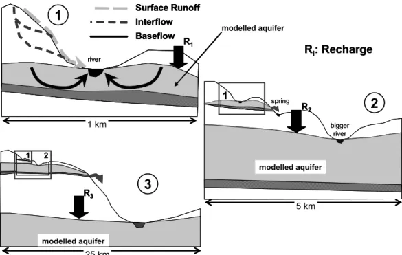
The scale dependency of definitions and the view point of the definitions identified so far (Figs. 3, 4) imply that the second process of interest, which is baseflow (see Fig. 2), should show analogous dependencies. The problem of find-ing a “true” definition for baseflow is explained schemati-cally in Fig. 6.

According to Fig. 6 the definition of baseflow, depends on:

a) the river (stream order, gauge etc.) that is considered in the hydrological model (less relevant if the model is merely conceptual),

b) the aquifer or aquifers described by the groundwater flow model and

c) the scale, the discretisation and the context of the mod-els.

Whereas in a conceptual hydrological model it is com-pletely irrelevant where baseflow comes from (it is just a “slow” runoff component) baseflow in a groundwater flow model must be exactly the volume of water flowing into an explicitly defined river, that infiltrated from the explicitly de-fined aquifers of the groundwater flow model. The same applies for groundwater recharge: Recharge R1 in Fig. 6 is not equal to recharge R3 and therefore not applicable as recharge in a groundwater model that considers only the large scale regional aquifer shown at the bottom of Fig. 6. Each “‘recharge” and “baseflow” has to be related to specific aquifers.

5 Conclusions

In this short discussion, some common problematic aspects of coupling groundwater flow models and hydrological mod-els (in a broader sense) were described. Coupling of such models is required in IWRM and Global Change research; furthermore it becomes apparent that the demand for model coupling rises with the size of the model area and the length of the period that is simulated. It was shown that the two main processes that connect surface and subsurface hydro-logical systems are groundwater recharge and baseflow (as-sumed here to be a synonym to groundwater runoff). Conse-quently it was stated that these two processes can be used to couple surface and subsurface models, i.e. hydrological and groundwater flow models. Groundwater recharge is an out-put of hydrological models and forms an inout-put (time variant boundary condition) for groundwater flow models. Baseflow is calculated by groundwater flow models and is used as an input for hydrological models.

In a next step, it was shown that the definition and mean-ing of both groundwater recharge and baseflow depend on disciplinary view points and additionally on the scale, dis-cretisation and context of the modelling task. Groundwater recharge as often defined in SVAT models is not necessar-ily the same as groundwater recharge required by a regional groundwater flow model. Baseflow calculated by a ground-water flow model is not necessarily the baseflow a concep-tual hydrological or a hydraulic river model assumes. It is therefore necessary to define these exchange processes and variables (and how they are calculated and used) very care-fully in all stages of model development and calibration in order to avoid severe modelling errors.

70 R. Barthel: Common problematic aspects of coupling hydrological models Baseflow Interflow Surface Runoff river 1 modelled aquifer spring bigger river 2 1 modelled aquifer 1 2 25 km 5 km 1 km

1

2

3

R

: Recharge

1

2

3

R

: Recharge

Figure 6: Scale and context dependency of groundwater-related hydrological processes.

According to Figure 6 the definition of baseflow, depends on:

a) the river (stream order, gauge etc.) that is considered in the hydrological model (less relevant if the model is merely conceptual),

b) the aquifer or aquifers described by the groundwater flow model and c) the scale, the discretisation and the context of the models.

Whereas in a conceptual hydrological model it is completely irrelevant where baseflow comes from (it is just a ‘slow’ runoff component) baseflow in a groundwater flow model must be exactly the volume of water flowing into an explicitly defined river, that infiltrated from the explicitly defined aquifers of the groundwater flow model. The same applies for groundwater recharge: Recharge R1 in Figure 6 is not equal to recharge R3 and therefore not applicable as recharge in a

groundwater model that considers only the large scale regional aquifer shown at the bottom of Figure 6. Each ‘recharge’ and ‘baseflow’ has to be related to specific aquifers.

14

Fig. 6. Scale and context dependency of groundwater-related hydrological processes.

A source of severe problems in coupling surface (unsatu-rated flow) and subsurface (unsatu(unsatu-rated flow) models is the fact that the unsaturated zone – in particularly on the regional scale – can be of considerable thickness (up to 1000 m and more). What is defined as the unsaturated zone depends of course always on the scale of the problem (see Fig. 5). Apart from the temporal effects this has on percolation, horizontal flow within this zone can lead to the result that water per-colating through the upper part of the unsaturated zone (1 to 10 m) will never or only partly reach the aquifer of interest. It is partly because this zone is inaccessible for measurements and partly because no branch of hydrological sciences feels responsible, that processes in this deep unsaturated zone (or transfer zone) are treated in a highly simplified or concep-tual manner, no matter how sophisticated the models for the zones above or below might be.

From these considerations, extensive conclusions can be drawn. The relatively new concept of IWRM as well as Global Change research have raised the demand for mod-els that can be applied on the regional scale and that allow an integrated view of all processes. Until now, most inte-grated (coupled) modelling approaches are based on the cou-pling of existing modelling concepts. Existing models are usually designed for a specific purpose and a specific scale. They follow a certain approach of process descriptions by including and calculating variables in a characteristic way. The problematic aspect when coupling such existing mod-els is the question of how to make them work together in a consistent way. A review of available models in particular

for groundwater flow simulation shows that the “old”, well-established, well-validated and quite often relatively simple models that would be appropriate for the use on the large scale are very problem-specific and therefore not suitable for integration. On the other hand, newer model concepts, es-pecially in the groundwater field, are much better suited for integration as they often can describe saturated as well as un-saturated flow. However, they are very parameter/variable demanding and are therefore not suitable for application on a regional scale.

Finally these considerations lead to the question of whether it always makes sense to follow the approach of coupling existing models in integrated modelling? A desirable alternative would be the development of new, fully integrated (holistic) concepts that are appropriately designed for the requirements of IWRM on a large scale. If this alternative proves impractical in view of the urgent demand for ready-to-use concepts, new sectoral model concepts customized for the application in integrated systems on the regional scale should be developed.

Edited by: R. Barthel, J. G¨otzinger, G. Hartmann, J. Jagelke, V. Rojanschi, and J. Wolf

Reviewed by: anonymous referees

References

Andres, G. and Egger, R.: A new tritium interface method for de-termining the recharge rate of deep groundwater in the Bavarian Molasse Basin, J. Hydrol., 82(1/2), 27–38, 1985.

Bergstr¨om, S.: The HBV model, in: Computer Models of Water-shed Hydrology, edited by: Singh, V. P., Water Resources Pub., Littleton, CO, 443–476, 1995.

Bronstert, A., Carrera, J., and Kabat, P.: Coupled Models for the Hydrological Cycle Integrating Atmosphere, Biosphere and Pe-dosphere, 240p., ISBN 3540223711, Berlin, 2005.

de Vries, J. J. and Simmers, I.: Groundwater recharge: an overview of processes and challenges, Hydrogeol. J., 10, 5–17, 2002. Harter, T. and Hopmans, J. W.: Role of Vadose Zone Flow

Pro-cesses in Regional Scale Hydrology: Review, Opportunities and Challenges, in: Unsaturated Zone Modeling: Progress, Applica-tions, and Challenges, edited by: Feddes, R. A., de Rooij, G. H., and van Dam, J. C., Kluwer, 179–208, 2004.

Halford, K. J. and Mayer, G. C.: Problems associated with estimat-ing ground water discharge and recharge from stream-discharge records, Ground Water, 38(3), 331–342, 2000.

Lemmel¨a, R. and Tattari, S.: Applications of transfer function and conceptual pulse models to the study of groundwater level fluc-tuation, Geophysica, 24(1–2), 33–46, 1988.

McDonald, M. G. and Harbaugh, A. W.: A modular three-dimensional finite-difference ground-water flow model, Techni-cal report, U.S. Geol. Survey, Reston, VA, USA, 1988.

Rauert, W., Wolf, M., Weise, S. M., Andres, G., and Egger, R.: Isotope-hydrogeological case study on the penetration of pollu-tion into the deep Tertiary aquifer in the area of Munich, Ger-many, J. Contaminant Hydrol., 14(1), 15–38, 1993.

Sanford, W.: Recharge and groundwater models: an overview, Hy-drogeol. J., 10, 110–120, 2002.

Scanlon, B. R., Healy, R. W., Cook, P. G.: Choosing appropriate techniques for quantifying groundwater recharge, Hydrogeol. J., 10, 18–39, 2002.

Seibert, J.: Multi-criteria calibration of a conceptual runoff model using a genetic algorithm, Hydrol. Earth Syst. Sci., 4(2), 215– 224, 2000.

Tallaksen, L. M.: A review of baseflow recession analysis, J. Hy-drol., 165, 349–370, 1995.

Tankersley, C. D., Graham, W. D., and Hatfield, K.: Comparison of univariate and transfer function models of groundwater fluctua-tions, in: Water Resour. Res., 29(10), 3517–3533, 1993. Vogel, R. M. and Kroll, C. N.: Estimation of Baseflow Recession