Applications of Optimization to Shale Oil and Gas
Monetization
by
Siah Hong Tan
B.S., Johns Hopkins University (2011)
S.M., Massachusetts Institute of Technology (2013)
Submitted to the Department of Chemical Engineering
in partial fulfillment of the requirements for the degree of
Doctor of Philosophy in Chemical Engineering Practice
at the
MASSACHUSETTS INSTITUTE OF TECHNOLOGY
June 2017
MASS-ACHUSETTSINSTTUTE OF TECHNOLOGYJUN 19 2017
LIBRARIES
ARCHIVES
@
Massachusetts Institute of Technology 2017. All rights reserved.
Author..
Certified by.
Accepted by...
Signature redacted
.
...
Department of Chemical Engineering
May 5, 2017
Signature redacted
Paul I. Barton
Lammot du Pont Professor of Chemical Engineering
Thesis Supervisor
Signature redacted
Daniel Blankschtein
Herman P. Meissner (1929) Professor of Chemical Engineering
Applications of Optimization to Shale Oil and Gas
Monetization
by
Siah Hong Tan
Submitted to the Department of Chemical Engineering on May 5, 2017, in partial fulfillment of the
requirements for the degree of
Doctor of Philosophy in Chemical Engineering Practice
Abstract
This thesis addresses the challenges brought forth by the shale oil and gas revolution through the application of formal optimization techniques. Two frameworks, each addressing the monetization of shale oil and gas resources at different ends of the scale spectrum, are developed. Importantly, these frameworks accounted for both the dynamic and stochastic aspects of the problem at hand.
The first framework involves the development of a strategy to allocate small-scale mobile plants to monetize associated or stranded gas. The framework is applied to a case study in the Bakken shale play where large quantities of associated gas are flared. Optimal strategies involving the continuous redeployment of plants are analyzed in detail. The value of the stochastic solution with regards to uncertainty in resource availability is determined and it indicates that mobile plants possess a high degree of flexibility to handle uncertainty.
The second framework is a comprehensive supply chain optimization model to determine optimal shale oil and gas infrastructure investments in the United States. Assuming two different scenario sets over a time horizon of twenty-five years, the features of the optimal infrastructure investments and associated operating decisions are determined. The importance of incorporating uncertainty into the framework is demonstrated and the relationship between the stability of the stochastic solution and the variance of the distribution of future parameters is analyzed.
The thesis also analyzes the Continuous Flow Stirred Tank Reactor (CFSTR) equivalence principle as a method for screening and targeting favorable reaction path-ways, with applications directed towards gas-to-liquids conversion. The principle is
found to have limited usefulness when applied to series reactions due to an unphys-ical independence of the variables which allows for the maximization of production of any intermediate species regardless of the magnitude of its rate of depletion. A reformulation which eliminates the unphysical independence is proposed. However, the issue of arbitrary truncation of downstream reactions remains.
Thesis Supervisor: Paul I. Barton
Acknowledgments
This thesis is the product of a labor of love. Nevertheless, its completion could not have been achieved without the help of several key individuals. First, I would like to thank my research advisor, Professor Paul Barton. What I appreciate most about Paul is that he has given me the freedom to chart my own path in research while ensuring that the quality of research is kept to high standards. To him, no question is too challenging to tackle, and he places his trust and patience in me to find a way. Through this process, I have grown to become a more fearless and thoughtful researcher who takes pride in getting things done right.
I would also like to thank my thesis committee members, Professors Robert Arm-strong and William Green, who have provided me with invaluable feedback on my work and gave me advice on how to proceed at each stage of this journey.
My thanks goes out to my fellow lab members at the Process Systems Engineering Laboratory. I appreciate the camaraderie and intellectual discussions that very much make our lab a special place. Special thanks goes out to Harry, Jose, and Rohit, who started the program with me. They are not only great labmates, but also great friends outside of the lab.
My thesis could not have been complete without the support of a close group of friends. Karthick and Sue Zanne, thanks for reminding me of home with our makan sessions. Kenneth, Marcus, Qinyi and Sheng Rong, thanks for all the fun and laughter during my early years. My thanks also goes out to Boon, Jon, Mila, Ming Qing and Rushabh for being great company at various stages of my time at MIT. Here's also a shout-out to my core team at Sloan - Gal, Galen, Maddie, Michael, Priyanka and Scott - fine individuals with whom I had the pleasure of working. Finally, my heartfelt thanks goes out to my good buddy Adriano, who taught me more about
life and business than the classroom ever could.
The MIT ecosystem of faculty and students is truly unparalleled in quality. Bril-liance can be found in every corner of the campus, be it in the classrooms, labs or lecture halls. Yet, this brilliance is often tempered with kindness and humility. I feel myself very fortunate to have been a part of this community. Definitely, I have grown to become a better version of myself in more ways than one. To all my coursemates, professors, lecturers and administrative and support staff with whom I have ever crossed paths, thank you for all that you have done.
Finally, thank you, Dominique, for being all that you are. To my parents, thank you for all the love and support you have given me not only for these few years, but for my entire life. Thank you for believing in me. This thesis is dedicated to you.
Contents
1 Introduction 23
1.1 B ackground . . . . 23
1.2 Small-scale mobile plants . . . . 26
1.3 Large-scale infrastructure investments in the United States . . . . 28
1.4 Mixed-integer linear programming . . . . 31
1.5 CFSTR equivalence principle . . . . 32
1.6 T hesis outline . . . . 33
2 Small-Scale Mobile Plants: Bakken Shale Play 35 2.1 Problem description and challenges . . . . 36
2.2 Mathematical formulation . . . . 39
2.3 Case study on the Bakken shale play . . . . 46
2.3.1 O verview . . . . 46
2.3.2 Technologies . . . . 47
2.3.3 Production curves . . . . 55
2.3.4 M arkets . . . . 59
2.3.5 Supply, price and demand projections . . . . 61
2.4 Concluding remarks . . . .
3 Small-Scale Mobile Plants: Addressing Uncertainty 3.1 Motivation . . . .
3.2 Stochastic formulation . .
3.3 Scenario generation . . . .
3.3.1 Supply . . . . 3.3.2 Demand and prices 3.4 Results and discussion . . 3.5 Concluding remarks . . . .
4 Shale Oil and Gas Investments in the United 4.1 Problem description and methodology . . . . . 4.1.1 General framework . . . . 4.1.2 Time horizon . . . . 4.1.3 Scenario sets . . . . 4.1.4 Sources . . . . 4.1.5 Plants . . . . 4.1.6 Markets . . . . 4.1.7 Transportation . . . . 4.2 Model formulation . . . . 4.2.1 Index sets . . . .
4.2.2 Sets constructed from index sets . . . .
4.2.3 Decision variables . . . . 4.2.4 Constraints . . . . 4.3 Results and discussion . . . .
States 73 77 78 79 83 85 87 87 98 99 100 100 102 103 104 107 116 123 132 132 133 135 137 144 . . . . . . . . . . . . . . . . . . . . . . . . . . . .
4.3.1 Computational results . . . 144 4.3.2 Profitability . . . 145 4.3.3 Investm ents . . . 147 4.3.4 Resources utilized . . . 153 4.3.5 Commodities delivered . . . 155 4.3.6 Transportation utilized . . . 158
4.3.7 Stochastic versus deterministic optimal investment decisions . 158 4.3.8 Variations in the degree of uncertainty . . . 166
4.3.9 Summary of results . . . 172
4.4 Concluding rem arks . . . 173
5 Examination of the CFSTR Equivalence Principle 175 5.1 Introduction . . . 176
5.2 Applying the CFSTR equivalence principle to a series reaction . . . . 181
5.3 A reformulation of the CFSTR equivalence principle . . . 183
5.4 Concluding remarks . . . 189
6 Conclusions 191 6.1 Summary and future work . . . 191
A Supplementary Material: Small-Scale Plants 193
B Supplementary Material: U.S. Investments 205
List of Figures
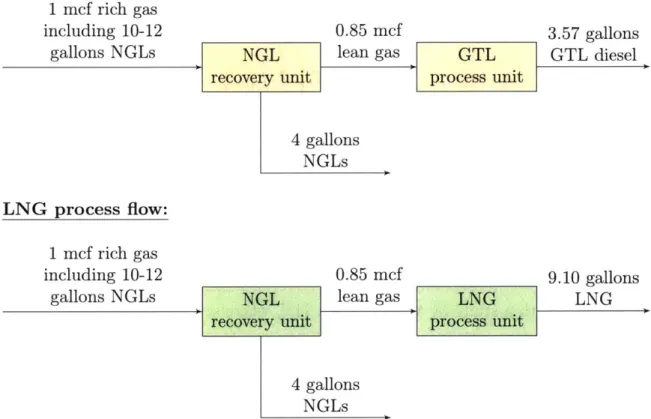
2-1 General simplified illustration of the dynamic mobile plant allocation problem to monetize associated or stranded gas. . . . . 38 2-2 Flow diagrams showing compositions of streams for the modular GTL
and LNG technologies under consideration. Flow rates are expressed on a 1 mcf feed rich gas basis. . . . . 48 2-3 Capital cost curve of GTL plants in actual implementation or in
lit-erature studies. . . . . 51 2-4 Capital cost curve of LNG plants in actual implementation or in
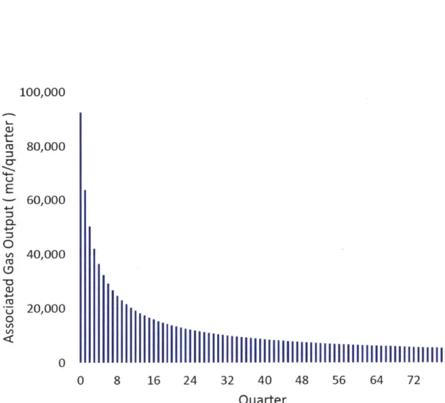
lit-erature studies. . . . . 52 2-5 Quarterly production curve of associated gas at a gas source under
consideration in the Bakken field. . . . . 58 2-6 Number of gas sources coming online per quarter. . . . . 63 2-7 Demand and price forecasts generated at a selected market for each
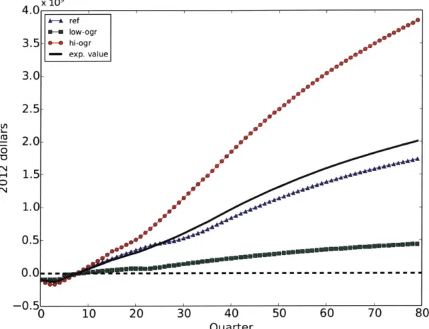
product under the Reference case. The complete set of forecasts for every market can be found in the Supplementary Material. . . . . 66 2-8 Cumulative NPV determined by solving the dynamic allocation of
2-9 Optimal plant deployment decisions at several points in the time hori-zon. Each cell in the grid represents a gas source with its correspond-ing gas flow rate. The presence of a square in the cell indicates that a plant has been deployed at that gas source for the current point in time. 69
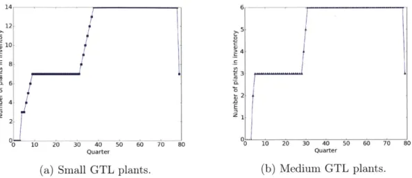
2-10 Number of plants in inventory over time. Plants of other types and sizes were not purchased. . . . . 71
3-1 Supply characteristics generated for the various scenarios under con-sideration: Reference (ref), Low Oil and Gas Resource (low-ogr) and
High Oil and Gas Resource (hi-ogr) . . . . 86
3-2 Demand and price forecasts generated at selected markets for the var-ious scenarios under consideration: Reference (ref), Low Oil and Gas Resource (low-ogr) and High Oil and Gas Resource (hi-ogr). The com-plete set of forecasts for every market is found in the Supplementary M aterial. . . . . 88
3-2 Demand and price forecasts generated at selected markets for the var-ious scenarios under consideration: Reference (ref), Low Oil and Gas Resource (low-ogr) and High Oil and Gas Resource (hi-ogr). The com-plete set of forecasts for every market is found in the Supplementary M aterial. . . . . 89
3-3 Cumulative ENPV and NPV for every scenario, determined by solving the stochastic program for the dynamic allocation of mobile plants. Scenarios: Reference (ref), Low Oil and Gas Resource (low-ogr) and
3-4 Optimal plant deployment decisions at several points in the time hori-zon for the Reference case. Each cell in the grid represents a gas source with its corresponding gas flow rate. The presence of a square in the cell indicates that a plant has been deployed at that gas source for the current point in tim e. . . . . 91
3-5 Plant deployment decisions at several points in the time horizon for the Low Oil and Gas Resource case. Each cell in the grid represents a gas source with its corresponding gas flow rate. The presence of a square in the cell indicates that a plant has been deployed at that gas source for the current point in time. . . . . 92
3-6 Plant deployment decisions at several points in the time horizon for the High Oil and Gas Resource case. Each cell in the grid represents a gas source with its corresponding gas flow rate. The presence of a square in the cell indicates that a plant has been deployed at that gas source for the current point in time. . . . . 93
3-7 Number of plants in inventory over time. LNG plants were not pur-chased .. . . . . 94
4-1 General framework of the supply chain in study. The flows of com-modities are represented with arrows. Resources from shale oil and gas sources can either be sold directly to the markets or undergo a con-version or upgrading process at different plants, where the resulting products are then sold to the markets. Variation of parameter values in different time periods and the uncertainty of future predictions are also incorporated into the framework. Constraints and an objective function are imposed with the formulation of an optimization problem. The circles containing 'I' and '0' refer to possible investment decisions and operating decisions respectively, made at either the nodes or arcs
of the supply chain. . . . 100
4-2 Locations of the seven sources in this study. . . ... . . . 105
4-3 Plant technologies under consideration and their associated inputs and outputs. ... ... .. .. .. ... ... . . . .... .109
4-4 Plant technologies under consideration and their associated inputs and outputs. ... ... 112
4-5 Cumulative Expected Discounted Cash Flows for each scenario set. 146 4-6 Cumulative Expected Discounted Cash Flows for each scenario set. 148 4-7 Optimal investments for each scenario set. . . . 149
4-8 Plant and pipeline investments for GDP scenario set. . . . 151
4-9 Plant and pipeline investments for Oil Price scenario set. . . . 152
4-10 Resources utilized for each scenario set. . . . 154
4-11 Commodities delivered for GDP scenario set. . . . 156
4-12 Commodities delivered for Oil Price scenario set . . . 157
4-13 Transportation utilized for GDP scenario set. . . . 159
4-15 Plant investm ents. . . . . 4-16 Pipeline investm ents. . . . . 4-17 The degree of uncertainty of scenario projections were varied by
per-turbing the parameters of High and Low scenarios from their original values, while keeping the Reference scenario invariant. . . . . 4-18 Optimal ENPV variations with the level of perturbation of scenario
projections from their original values. . . . . 4-19 Stochastic plant investments change depending on degree of
pertur-b ation. . . . . 4-20 Stochastic pipeline investments change depending
turbation. . . . .
5-1 Arbitrary reactor formulation. . . . . 5-2 CFSTR equivalent formulation. . . . .
on degree of per-170
. . . 184
. . . 186
Demand forecasts for all GTL diesel markets. Demand forecasts for all GTL diesel markets. Demand forecasts for all GTL diesel markets. Price forecasts for all GTL diesel markets. . . Demand forecasts for all LNG markets. . . . . Price forecasts for all LNG markets. . . . . Demand forecasts for all NGLs markets. . . . Price forecasts for all NGLs markets. . . . . . . . . 199 . . . 200 . . . 201 . . . 202 . . . 203 . . . 203 . . . 204 . . . 204 162 164 167 168 169 A-i A-i A-i A-2 A-3 A-4 A-5 A-6
List of Tables
1.1 Different dimensions of scope in which a supply chain optimization can vary in its extent of comprehensiveness. Having a more compre-hensive model is ideal, but has to be balanced with considerations of
computational tractability. . . . . 30
2.1 Basic characteristics of the GTL and LNG mobile plants under con-sideration . . . . 53
2.2 Capital costs for GTL and LNG mobile plants. . . . . 56
2.3 Operating costs for GTL and LNG mobile plants. . . . . 56
2.4 Bakken well production characteristics and assumptions. . . . . 57
2.5 Type and number of markets for GTL diesel, LNG and NGLs products and associated shipping costs. . . . . 61
4.1 Scenarios corresponding to each scenario set (GDP and Oil Price). . . 104
4.2 Initial production rates of resources at the sources at the beginning of 20 15 . . . 106
4.3 Summary of plant characteristics. Corresponding units are indicated in brackets. Abbreviations for products: G (gasoline), K (kerosene), D (diesel), R (residual fuel oil), L (liquefied natural gas). . . . 117
4.4 Types of commodities accessible to respective markets. . . . 118 4.5 Types of commodities carried by each mode of transportation. ... 124 4.6 Pipeline capacities available for investments. Abbreviations for flows:
s-p (source-to-plant), s-m (source-to-market), p-m (plant-to-market). 126 4.7 Transport costs for transportation modes in the study. . . . 130 4.8 Optimal NPVs (in $B) over entire time horizon for each scenario and
expected value in each scenario set. . . . 145 4.9 Outlooks and associated nominal scenarios. . . . 161 4.10 Optimal objective values of the recourse problems and initial
invest-ments arising from fixing the optimal investment decisions generated from various ex-ante outlooks. . . . 165
5.1 Reformulated problem 5.23 implemented in BARON 11.9.1, where the
upper bound of Vk is set at 1 x 10³. The optimal value of the objective
function is shown as a function of the number of CFSTRs. . . . 189
A. 1 Reported capital costs of GTL plants in actual implementation or in literature studies. . . . 194 A.2 Reported capital costs of LNG in actual implementation or in
litera-ture studies. . . . 195 A.3 Breakdown of fixed operating costs for small-scale plants. *Rounded
to nearest thousand. . .. .. ... . . . ... 196 A.4 Breakdown of variable operating costs for small-scale plants . . . 197 A.5 Markets of various products under study. Census Divisions
abbrevia-tions: ENC = East North Central, MTN = Mountain, WNC = West North Central, WSC = West South Central. . . . 198
B.1 Assumptions for the AEO 2015 Cases. Taken from
[1]
. . . 206B.2 Geographical coordinates of sources . . . 207
B.3 Mapping of plays to wet source for the determination of NGL content. Basins/plays referenced from
[2]
.. . . . 208 B.4 Scores assigned to land cover type from the National Land CoverDatabase dataset. Detailed descriptions of the land cover classifica-tions can be found at
[3].
. . . 209B.5 Scores assigned to land ownership type from the U.S. National Atlas Federal and Indian Land Areas dataset. . . . 209
B.6 Geographical coordinates of candidate plant locations . . . 210
B.7 Process cost function parameters for process units in a hydroskimming refinery. Taken from [4]. . . . 211
B.8 Mapping of commodities in study to exported products classification in EIA's Exports by Destination data. . . . 213
B.9 Initial demand values of NGLs and refined products for each foreign market. Units are in MMB/year. . . . 213
B.10 Initial prices used for price series in foreign markets. . . . 214
B.11 AEO 2015 series used for determining the future evolution of corre-sponding parameter values at the sources. . . . 215
B. 12 AEO 2015 series used for determining the future evolution of corre-sponding parameter values at the markets. Asterisks represent spe-cially constructed series, as described in the body of the paper. * : Appropriately apportioned quantities of the AEO 2015 Natural Gas : Volumes : Exports : Liquefied Natural Gas Exports demand series, according to relative foreign consumption ratios in IEO 2013 Refer-ence Case. ** : 'Mexico Blend' prices, which are the average of Brent and W TI prices. . . . 216 B.13 List of U.S. oil pipeline projects used for determining oil pipeline cost
curve. ... ... ... .. .. .... . . .. .. .. . .... .218
B.14 Regression coefficient estimates for log-log relation between pipeline capital costs per length and capacity. Standard errors are shown in parentheses. . . . . 218
B. 15 U.S.-Mexico Border Points used in determining pipeline and rail trans-portation routes to Mexico. . . . 221 B.16 Representative ports of U.S. and Foreign Coasts. . . . 221
Chapter 1
Introduction
1.1
Background
The main theme of this thesis is the application of optimization techniques with the aim of optimal monetization of oil and gas from unconventional resources. The discovery of large reserves of shale oil and gas in many locations worldwide and the technological advances that have made it possible to exploit them has presented an unprecedented economic opportunity. This revolutionary development in the global energy arena has been led largely by activity in the United States. From 2008 to 2013, U.S. crude oil production grew from 5.0 to 7.4 million barrels a day, and U.S. dry natural gas production grew from 20.2 to 24.3 trillion cubic feet per year
[5].
The work of this thesis began at a time when the shale revolution was transi-tioning from a focus on upstream activities towards that on mid- and downstream activities. Great strides in increasing the efficiency of shale oil and gas production and the management of production sites were already being made, and the ques-tion of the day turned towards analyzing the possible ways in which the growing
abundance of shale oil and gas could be monetized.
The analysis of shale oil and gas monetization involves the simultaneous consid-eration of numerous factors, including technological options, scales of production, availability of existing infrastructure, nature of production at sources, nature of markets, economic parameters of prices, demand and supply of resources and end products, transportation options, time horizon, and uncertainty of future conditions. With the multitude of options, heuristic approaches to determine the best options for monetization are likely to lead to sub-optimal results.
The aim of this thesis seeks to address this issue through formal optimization techniques. Formalized optimization frameworks can handle complexity with relative ease. The development of efficient algorithms and formulations, combined with the rapid increase in computational power of modern computers over the past decades, has now made it possible to solve once-intractable problem instances containing tens of millions of variables and constraints. The holistic yet granular nature of an optimization framework allows it to uncover optimal solutions which might not be accessible by heuristic-based analyses.
The heart of this thesis' analysis is centered around the twin issues of scale and risk and their associated trade-offs. On one hand, operating at larger scales allows for the benefits of economies of scale. On the other, the large capital outlay and lengthy development times might pose a significant risk for investors due to consid-erable uncertainty in the future demand, supply and prices at the time at which an investment decision is being made.
As the scale of operation decreases, there is a distinct discontinuity in the con-ceptualization of the mode of operation of plants. The main difference is that below a certain operational scale, individual plants gain the ability to be moved to dif-ferent locations during their lifetime. This discontinuity in the mode of operation
leads to distinct formulations of the optimization models and their specific realms of application. As such, the work of this thesis is organized around this distinction.
The application of optimization techniques to solve problems related to shale oil or gas in the research community is still relatively new. A brief overview of the relevant studies performed thus far are given here.
Martin and Grossmann
[6]
presented a superstructure optimization approach to produce liquid fuels and hydrogen from switchgrass and shale gas in a facility. Cafaro and Grossmann [7] optimized the design and operation of supply chain networks at shale gas drilling sites. Yang et al.[8]
optimized water management operations during shale gas production to maximize profits. An extension to consider both strategic design decisions and environmental objectives in the optimization of water management during shale gas production was provided by Gao and You[9].
The same authors also optimized a shale gas and water supply chain network from well sites to power plants and performed a life-cycle analysis of electricity generated from shale gas [10].In a series of papers, Knudsen and Foss [11] optimized the production from a set of late-life wells at a shared production pad to avoid well liquid-loading. The formulation was extended to multiple pads and solved using a Lagrangian relaxation based decomposition scheme [12]. Later, the scheduling problem was extended to consider the operation of the wells to supply electric power
[13].
Bistline [14] explored how uncertainties in natural gas prices and future climate policies impacted economic and environmental outcomes in the U.S. power sector with a two-stage stochastic programming formulation.1.2
Small-scale mobile plants
Large upfront investments preclude the tapping of stranded gas reserves, which are reserves that are either too small or too physically inaccessible to be economically exploitable. A recent survey by Attanasi and. Freeman [15] of the gas fields in the world excluding the U.S. estimated that only around 12.2% of the gas fields tabulated were larger than 1.54 tcf in size. In contrast, as indicated by Velocys [16], the remaining fields which would be considered too small to monetize by traditional large-scale technologies might be accessible to medium- to small-scale technologies.
Stranded gas can also arise from the lack of infrastructure access despite the field having a large size. A pertinent example in the United States is the gas associated with the production of shale oil at liquids-rich fields, such as the Bakken shale field in North Dakota. In 2013, Ford and Davis
[17]
estimated that 33% of the natural gas produced at the Bakken was not marketed, where most gas not marketed was flared.Recent concepts for implementing gas-to-liquids (GTL) and liquefied natural gas (LNG) technology at a small-scale and modular level have the game-changing po-tential to shift the paradigm away from large capital expenditures and one fixed lo-cation. These proposed plants are currently in the early stages of commercialization by several companies in the oil and gas industry, including GE Oil & Gas [18], Com-pactGTL [19] and Velocys [20]. These technologies involve pre-manufacturing each process unit as compartmentalized, individual modules which can then be shipped to the site of interest and assembled together in minimal time to form the entire plant. Additionally, plants can be quickly disassembled into their individual modules and redeployed at other sites, affording them the benefit of mobility. This mobility will allow them to respond quickly to changes in conditions that might affect their
prof-itability. This could include economic factors such as large changes in the price of both the raw gas and its associated products, and supply shocks arising from the steep decline curves typically observed with unconventional sources of gas. For ex-ample, a study by Hughes in 2013 [21] concluded that wells in the top five U.S. shale plays typically produced 80-95% less gas after three years. Although the commercial availability of modular plants is limited at the time of writing, there has been a grow-ing interest in evaluatgrow-ing them for purposes of monetizgrow-ing stranded or associated gas from both conventional and nonconventional sources.
In view of these promising claims, it would be both useful and informative for industry players to have access to a framework that optimally utilizes these small-scale, mobile technologies to monetize stranded or associated gas. To this aim, this thesis develops a multi-period strategy for the optimal allocation of these technologies under time-varying supplies of gas in locations where stranded or associated gas is present and time-varying prices of and demand for the various products in their respective markets.
Prior to this work, the application of optimization to analyze small-scale mobile plants has not been investigated in literature, to our knowledge. However, ideas on problem formulation are similar in the context of the unit commitment problem. For example, in the case of a hydro-thermal system, decisions are made to operate thermal units and pumped hydro storage plants, which can be turned off and on at certain time points [22, 23].
1.3
Large-scale infrastructure investments in the
United States
With high levels of growth of shale oil and gas production, there has been an accom-panying increase in capital spending on midstream and downstream infrastructure
[24].
These infrastructure investments primarily aim to provide greater access to shale plays which previously lacked connections and direct the resources to locations where additional demand could be served.Unfortunately, making infrastructure investments in the oil and gas industry is rarely a straightforward affair. Because of the large sizes of investments, regulatory and geopolitical challenges, and considerable uncertainty in future resource prices, projects often face schedule delays and cost overruns
[25].
In severe cases, the original intentions behind the investments might have to be abandoned. A pertinent example would be the over-investment in LNG import terminals in the early 2000s, when the general expectation was that of significant declines in future U.S. natural gas production [261.To deal with the challenges associated with oil and gas infrastructure investments, a formalized framework in which to analyze these investments is required. This thesis develops a framework which assumes a comprehensive, high-level view of making optimal shale oil and gas investments in the context of current and future projections of supply, demand and prices of various commodities. This framework allows for a systematic study of the optimal types and levels of infrastructure investments, as well as the accompanying operational aspects of the supply chain.
The study continues the rich history of the application of optimization techniques to solve problems related to the management of supply chains. In particular, it can
be broadly associated to the study of facility location problems, where in general, optimal facility locations are to be determined to satisfy customer demand, with the objective of minimizing overall costs or maximizing overall profits. A review of the history of these problems is given by Owen and Daskin [271. A compilation of significant contributions to the field, as well as mention of potential areas for further research, was given by Melo et al. [28]. A review of supply chain optimization specifically applied to the field of energy, in particular, that involving hybrid feedstock processes, was contributed by Elia and Floudas [29]. In these reviews, the importance of the need for more future models to incorporate both stochastic and dynamic aspects was highlighted. Sahinidis [30] provided a review of optimization under uncertainty, which provides hints of how one might extend the traditional facility location problems to their stochastic counterparts.
Although there has been a long history of papers demonstrating the application of supply chain optimization, we believe that the study in this thesis possesses a scope that is unprecedented in existing literature. Table 1.1 shows the different extent in which a supply chain optimization framework can vary in terms of its comprehensiveness, and as indicated, the study in this thesis lies on the high side of comprehensiveness for all of the dimensions of scope explored. To the best of our knowledge, most papers in existing literature typically only possess the high side of comprehensiveness for one or two dimensions of scope at best, while the other dimensions remain on the low side of comprehensiveness.
In addition, to the best of our knowledge, there has been no comprehensive na-tionwide supply chain optimization model specific to shale oil and gas prior to this work. Our framework integrates the economic dynamics of the upstream, midstream and downstream sectors of the oil and gas industry in the U.S. and select foreign markets and takes into account both the time-varying projections of supply, demand
less comprehensive more comprehensive Scope Extent Midstream Downstream Structure Time periods Objective Uncertainty Geography Technologies Commodities Transportation Vt
Converging Diverging Multi-nodal
Single (Rate-based) Multiple
Cost-based Excluded VP Profits-based VI Included Vt
State Region Country International
Single Single Single Multiple Multiple Vt Multiple
Table 1.1: Different dimensions of scope in which a supply chain optimization can vary in its extent of comprehensiveness. Having a more comprehensive model is ideal, but has to be balanced with considerations of computational tractability.
and price parameters as well as the different scenario realizations of these parame-ters. The development of the model would achieve the aim of providing an accurate and timely guide towards making the best investment and operating decisions for monetizing shale oil and gas in the country moving forward.
1.4
Mixed-integer linear programming
The optimization frameworks developed in this thesis are formulated as mixed-integer linear programs (MILP), which have the following structure:
minimize cTi + dT y
subject to Ax
+
Dy = b,x E X n R+ ,
where x are nonnegative continuous variables and y are nonnegative integer variables. X and Y denote polyhedral sets containing x and y respectively. c, d are cost vectors for x and y, respectively. Ax + Dy = b are the coupling constraints between these variables.
In the context of the thesis, the continuous variables typically refer to the opera-tional decisions, whereas the integer variables typically refer to investment, location, or logical decisions.
Modern commercial solvers like CPLEX [31] and Gurobi [321 typically imple-ment a branch-and-cut method to solve the MILP. Many ways in which the solution procedure can be made more efficient are documented in literature, typically by de-veloping sharp formulations, formulating tight cuts, or decomposing the structure of
the problem into smaller subproblems
[33].
However, the effectiveness of these mod-ifications over a direct implementation of the fullspace formulation depends largely on a case-by-case basis among the instances examined.1.5
CFSTR equivalence principle
Chemical engineers often encounter reaction schemes with varying complexity and have an abundance of reactor and separator designs to choose from. This proves to be a formidable task, and a method for screening reaction schemes is often desired such that more attention can be focused on particular schemes that have comparatively higher productivities of a certain desired species. It was with this in mind that Fein-berg and co-workers developed a theory to determine an absolute and computable limit for the achievable production of any species for any arbitrary steady-state reactor-separator design, given the kinetics of the reaction network and a specified commitment of resources [34, 35]. Named the Continuous Flow Stirred Tank Reac-tor (CFSTR) equivalence principle, it asserts that the effluent of any steady-state reactor-separator design can be achieved arbitrarily closely by another steady-state design with arbitrarily sharp separations but in which the only reactor components are s + 1 ideal CFSTRs, where s is the rank of the underlying network of chemical reactions.
The CFSTR equivalence principle is atttractive because it has a simple form yet powerful applicability as a screening tool for potentially very complex reaction networks. In this thesis, distinct from the studies above, we explored the applicability of the principle to screen and target favorable reaction pathways, with applications directed towards gas-to-liquids conversion.
1.6
Thesis outline
The outline of the remainder of the thesis is as follows:
" Chapter 2 discusses an optimization framework for the dynamic allocation of small-scale mobile plants to monetize associated or stranded gas and its appli-cation to the Bakken shale play.
" Chapter 3 expands upon the previous chapter by incorporating uncertainty into the framework.
" Chapter 4 discusses a comprehensive supply chain optimization framework to determine optimal shale oil and gas infrastructure investments in the United States.
* Chapter 5 explores the screening of reaction networks using an optimization framework based on the CFSTR equivalence principle.
* Chapter 6 concludes.
" Appendix A provides Supplementary Material for Chapters 2 and 3.
" Appendix B provides Supplementary Material for Chapter 4.
* Appendix C provides the Capstone Paper, written during my studies at the Sloan School of Management.
Chapter 2
Small-Scale Mobile Plants: Bakken
Shale Play
Associated or stranded natural gas presents a challenge to monetize due to its low volume and lack of supporting infrastructure. Recent proposals for deploying mobile, modular plants, such as those which perform gas-to-liquids (GTL) conversion or produce liquefied natural gas (LNG) on a small scale, have been identified as possible attractive routes to gas monetization. However, such technologies are yet unproven in the marketplace. To assess their potential, we propose a multi-period optimization framework which determines the optimal dynamic allocation and operating decisions for a decision maker who utilizes mobile plants to monetize associated or stranded gas. We then apply this framework to a case study of the Bakken shale play. Our framework is implemented to determine the optimal net present value (NPV) which would be realized over a twenty-year time frame. Sensitivity studies on the technology costs and conversion inputs conclude that the profitability and viability of mobile technologies remain valid for a wide range of possible inputs.
2.1
Problem description and challenges
We will assume the role of a decision maker whose primary concern is to monetize natural gas in stranded fields or associated with the production of oil. When making decisions, the decision maker would have to consider the production characteristics unique to the field and choose among several technology options. These technologies convert natural gas into either higher-value products or a more transportable form, or both. Among the technology options available, two which have garnered the most interest due to their relative maturity are the gas-to-liquids (GTL) and liquefied natural gas (LNG) technologies.
GTL has recently gained attention due to the increased spread between the price of oil and natural gas, as noted by Hobbs and Adair [36] and Salehi et al. [37]. The GTL process converts natural gas into liquid fuel. There are three main parts to this process: 1) syngas generation, 2) Fischer-Tropsch (FT) synthesis, and 3) refining and upgrading.
In syngas generation, natural gas is first cleaned and then converted into syngas, which is a mixture of hydrogen and carbon monoxide. After the syngas has been generated, it undergoes FT synthesis where it is converted into longer chain hydro-carbons. Finally, after the FT synthesis step, the product is sent for refining and upgrading to meet final specifications.
GTL products are attractive not only because they are liquid fuels and can be easily transported, but also because they are virtually sulfur-free, as mentioned in studies by Wood et al. [38] and Salehi et al. [37]. The most promising product from the GTL process is GTL diesel. Also high in cetane number, it is ideal as a blendstock for refineries to adjust conventional diesel in production to meet specifications.
lique-faction of gas by cooling to cryogenic temperatures. Prior to cooling, the feed gas undergoes several treatment steps, such as filtration and removal of carbon dioxide, sulfur, mercury and water.
The value of LNG is that it significantly increases the energy density of natural gas, allowing it to be transportable for sale in distant markets. In the U.S., the most promising market for LNG is fuel for heavy-duty trucks or freight rail, as documented in a study by TIAX [39].
In addition, depending on the source of natural gas, there may be a significant presence of natural gas liquids (NGLs), ethane, propane, butane, etc., mixed in the wellhead gas. Such gas is termed "wet gas", and the NGLs are usually separated from the mixture because they possess substantial economic value. NGLs primarily serve as feedstock for the petrochemical industry or as fuel for heating and transportation purposes, as noted by Platts Price Group
[401.
Therefore, GTL and LNG technologies which take in wet gas as their feedstock should necessarily have a NGL separation unit.Applying these technologies to monetize stranded or associated gas poses a chal-lenge. First, the technologies have to be designed to be mobile, since the supply of gas at any fixed location would not last for very long. The mobility of the plants adds a dimension of complexity to the decision-making process. Although the idea of mobility generally allows plants to be more agile and thus suitable for capturing stranded gas, start-up and shut-down costs would be incurred every time a move is made. Thus, the company has to weigh the costs and benefits of continuing oper-ations at a certain location versus redeployment in the context of how the supply profile and the demands of its customers evolve over time. Second, because of the dynamic nature of gas supply and well availability, it is a challenge to determine the optimal number of mobile plants of each technology type to be purchased or sold at
each time point of the time horizon that would maximize profits.
Market Market Market
A A A
GTL
Available source Available source Depleted source
-LNG N LNG GTL
Anticipated source Anticipated source Available source Available source Available source vailable source
LNG Of P~
Market Market Market
GTL Inventory of plants B Inventory of plants B Inventory of plants B
I 1" period 2"d period 3'd period
to t2 Legend:
Product 1 flow
Progression of time Product 2 flow
Figure 2-1: General simplified illustration of the dynamic mobile plant allocation problem to monetize associated or stranded gas.
Figure 2-1 portrays a simplified illustration of the decision framework under con-sideration. In this example, there are three time stages, three gas sources, two technologies for mobile plants (GTL and LNG) and two markets. Depending on the time period, the gas sources might or might not have gas available to monetize in various quantities. At each time stage, the decision maker has to decide how many plants of each technology type and size to purchase or sell and where to locate ex-isting plants purchased in previous time stages, along with the appropriate levels of production to deliver the finished products to the markets. In Figure 2-1, we see that the decision in the first time period to purchase a GTL and an LNG plant and develop gathering systems at the gas sources is made in anticipation of more sources coming online in subsequent time periods. Once the plants have been constructed off-site and shipped to the site of operation in the second time period, they are then
available for the decision maker to deploy to the available gas sources. Subsequently, between the second and third time period, the gas source in which the GTL plant has been located becomes depleted. Hence, the decision is made to move the plant to another source where it can resume its operations profitably. All decisions are 'made with the goal of maximizing the net present value (NPV) of the project over
the entire time horizon.
2.2
Mathematical formulation
The problem is formulated as a multi-period MILP. A decision maker makes decisions
on a uniform grid t E
{O,
... , T} over a given time horizon. Based on the topology ofthe gas field and the production characteristics, the decision maker has access to a
number of gas sources i
E {1,
... , I}, which might or might not supply gas dependingon the point in time considered. At each source, the decision maker can choose to deploy a plant of type
j
C
{1,
. . ., J} in order to monetize the gas. The products arethen shipped and sold to various surrounding markets k E
{
1, ... , K}, each of whichhas a demand for a particular type of product 1
E
{1,...
, L}. In order to track theage of the plants at a given time t, we also record the time point at which the plant was purchased T
{,
... , t}.The optimization decisions are:
1. Decision to allocate plant of type j to source i at time t, denoted by yj, E
{o,
1}.2. Indicator of the presence of a gas gathering system at source i at time t, denoted
by z E {o, 1}.
4. Product delivery rate of product 1 from source i to market k at time t, denoted by w'k1 E R+.
5. Number of plants of type
j
purchased at time t, denoted by Buyt E Z+.6. Number of plants of type
j
which originally arrived in inventory at time 0 <T < t, sold at time t, denoted by Sell5 E Z+.
7. Inventory of plants of type j at time t, arriving in inventory at time 0 < T < t,
denoted by Irniv E Z+.
The decision maker has to make his or her decisions subject to the following constraints.
Once a decision has been made to develop a gathering system at source i at time t, the gathering system is available at that source for all subsequent time points:
zt zt+ , Vi, VO < t < T. (2.1)
A plant can only be deployed at a particular source if a gathering system had been developed at least
T
time periods prior, whereT
denotes the time necessary to construct the gathering system:y. < zh , Vij, Vt> T, and (2.2) y = 0, Vij, Vt < Tg. (2.3)
The inventory balance of plants has to be satisfied. Constraints (2.4) describes the inventory balance where r = t, (i.e., for plants that are brand new). In this case, the inventory of new plants are simply the number bought 'T time stages ago, where
7 denotes the construction time lag between the purchase of plants and their actual arrival in the inventory ready for deployment.
InV5T = BUY>, Vj, Vt ;> , VT= t, and (2.4)
InVt = 0, Vj, Vt < 7, VT = t.
Constraint (2.5) describes the inventory balances where T < t, which considers
plants which are at least one time point old. Here, the current inventory of plants bought at a particular previous time point is simply that carried forward from the previous inventory, less any plants that are sold.
InV> = Inv;-1 - Sellt, V j,t, Vr < t. (2.5)
The number of plants allocated to the sources cannot exceed the number of plants in the inventory. Note that we are indifferent to the purchase date of the plant and treat all plants as equally efficient for our allocation decisions:
t
y < Z nlV r, Vj, t. (2.6)
Each gas source is associated with a gas supply st. If a plant has been deployed at a gas source, the gas feed rate to the plant cannot exceed the gas supply from the source:
As <; sfy Vi, , s. (2.7)
the gas supply:
Zxt < st, Vi, t. (2.8)
Each plant type is associated with a capacity m. The feed to a plant cannot exceed the plant's capacity:
x,3 < mg y{, Vi, j, t. (2.9)
In addition, each plant type is associated with a minimum capacity that cannot be violated due to physical constraints on the equipment. This minimum capacity is determined by the turndown ratio, expressed as a fraction 7j of total capacity. Thus, if allocated, the feed to the plant cannot be below the plant's minimum capacity:
x ;> -yjn jyt, Vi, j, t. (2.10)
For each technology, we denote a conversion factor ay, to denote the proportion of gas feed which gets converted into an end product. Then, the total flow rate of a product exiting a source must equal the sum over all routes of shipment of that product to its markets:
OzI X 0JXJZWt 11 Vil lt. (2.11)
j k
k
Each market is associated with a demand dt. Then, if a market is chosen to be served, the total rate of products delivered to that market cannot exceed their
demand:
WtS < W tkI, Vk,l,t. (2.12)
The objective function of the decision maker is to maximize the net present value (NPV) of the project, given an appropriate discount factor r:
NPV = (1 + r)-t(Revt - Cost') (2.13)
t
where Rev' is the total revenue and Costt is the total cost at time t.
Rev' is defined as the sum of the following terms. The sale of all products, each
with a corresponding price ptl:
S
~~S
S5iic~i4
(2.14)
i j k 1
The gains obtained by salvaging a plant and its associated equipment. The
salvage value of a plant
j
purchased at time r, sold at time t, is denoted catt
S
a Sellit . (2.15)j T=0
Cost' is defined as the sum of the following terms. The total plant investment
costs, where each plant has an associated capital cost ceap,,:
The total gathering system investment costs, where each gathering system has
an associated capital cost Cgathercap. Note that because of Constraint (2.1), we are guaranteed that for each term cgathercap(Z4 - z- 1), with i fixed, there will be at most
one non-zero term across all values of t:
Cgathercap(Zt - (2.17)
The total startup costs of deploying plants to their sources. These costs include installation and assembly costs of the plant to the associated gathering system con-necting to the wells, as well as any lost revenue that occurs due to partial operation during the period. The following representation assumes that a plant can be set up within the time elapsed between two time points:
cstartjmaX{Yij - yj , 0}. (2.18)
i j
The total shutdown costs of removing plants from their sources. These costs include disassembly and removal costs of the plant from the associated gathering system connecting to the wells, as well as any lost revenue that occurs due to partial operation during the period. Again, the following representation assumes that a plant can be shut down within the time elapsed between two time points:
5
Cshutjmax{Y - y, O}. (2.19)i i
repre-sented by introducing auxiliary variables ,ijsti ,tart E R+ and the constraints:
y - yt I < 6t Vi
j,
t, (2.20) (2.21)Vil
j)tiwhich then allow (2.18) and (2.19) to be represented byEi Ej Csa'rt,jStt,,j and
Y Cosht,j 6s ,ij, respectively. Note that when t = 0, we set ytj-1 to 0.
The total operating costs of the plants. The operating costs are divided into fixed operating costs copFixed,j and variable operating costs
CopVar,j-CopFixed,jYzj, (2.22)
2 t
CopVarjXij . (2.23)
The total transportation costs of products from the plants to their markets. Ship-ping a product 1 from its source i to a market k incurs a per unit cost of cship,ikI. This cost primarily depends on the mode of transportation and the physical distance between the gas source and the market:
555
2 k I
t
Cship,ik1Wikl.
The total costs of wellhead gas fed to the plants. The spot price of the wellhead
gas is denoted by ptsi:
Pgas,iZij.
2 j
(2.25) (2.24) t-1 - t < 6t
In the case of associated gas otherwise flared if not monetized, Pgas,i = 0.
In short, we seek to maximize (2.13) subject to the constraints of Eqs. (2.1) to (2.12) and (2.20) and (2.21).
2.3
Case study on the Bakken shale play
2.3.1
Overview
The Bakken Formation is a wet shale formation occupying approximately 200,000 square miles within the Williston Basin, extending through various parts of North Dakota, South Dakota, Montana and the Canadian provinces of Manitoba and Saskatchewan. A detailed description of the formation was given by Wocken et
al. 141].
The rapid growth in oil production has also led to a significant production of associated gas. Despite attempts to develop infrastructure to gather, process and transmit the gas, this has proceeded at a much slower rate than that of production. The result has been a rapid increase in the amount of gas that is unable to be monetized and hence flared.
There are several unique aspects to consider when monetizing associated gas in the Bakken play: first, as analyzed by Mason [42], the production rate of a typical well operating on unconventional resources faces a very steep decline. As a result, the flow rates of associated gas might very quickly drop to levels which make the gas uneconomical to monetize. Second, as indicated by Wocken et al. [41], the associated gas arising from the Bakken is typically wet, and exists as a mixture of methane and NGLs. Therefore, when developing technology to be implemented in the Bakken, we
include an NGL separation unit in the process.
We adopt the role of a decision maker who faces a time horizon of twenty years, divided into quarterly time steps. The choice for twenty years corresponds to the typical lifespan of a mobile plant implementing the technologies that we considered
- GTL and LNG, each of three different sizes.
2.3.2
Technologies
Figure 2-2 shows the flow diagrams of the two systems considered, specifying flow rates and compositions of the feed gas and finished products. There are three sizes for each system considered in our study - small, medium and large. The sizes corre-spond to the capacity to process a feed rate of 500, 1,000, and 1,500 thousand cubic feet (mcf) of rich gas per day, respectively. Although in reality the gas composition can vary between the Bakken wells, we assumed a constant, representative gas com-position at 10 - 12 gallons of NGLs per 1 mcf of rich gas. This value was chosen to be in line with a study by Wocken et al.
1411,
where several options for monetiz-ing associated gas in the Bakken were discussed and assessed by a more qualitative approach.Each technology produces two high-value products: the "GTL process" produces NGLs and GTL diesel, while the "LNG process" produces NGLs and LNG. Although 10 - 12 gallons of NGLs is present per mcf of feed gas, the recovery of NGLs in the product stream can only be achieved at a rather low rate at 4 gallons per mcf of feed gas. This recovery rate was obtained from the Wocken et al.
[411
study. The low recovery rate was mainly due to the technological simplicity of the extraction unit, which operated as a two-stage compression and chilling process at -20 *F and 1,000 psi. Although not explicitly stated in the report, it could be that the technologicalGTL process flow:
1 mcf rich gas including 10-12
gallons NGLs
0.85 mcf 3.57 gallons
NGL lean gas GTL GTL diesel
recovery unit process unit
4 gallons NGLs 1 mcf rich gas including 10-12 gallons NGLs 0.85 mcf 9. 10 gallons NGL lean gas LNG LNG
recovery unit process unit
4 gallons
NGLs
Figure 2-2: Flow diagrams showing compositions of streams for the modular GTL and LNG technologies under consideration. Flow rates are expressed on a 1 mcf feed rich gas basis.
sophistication of the NGL extraction process was limited by size requirements. For the GTL process, a conversion factor of 1 mcf of lean feed gas to 0.1 barrel of GTL diesel product was used, which matches the values reported by Patel
[43]
and Wood et al.[381.
For the LNG process, we assumed an efficiency rate of 88%, as reported by Patel [431 and Garcia-Cuerva and Sobrino[44].
This corresponds to a conversion factor of 1 mcf of lean feed gas to 10.7 gallons of LNG. We then assumed that 85% of the rich gas flow rate is recovered as lean gas after the extraction of NGLs. This is again in line with the assumptions made by Wocken et al [41]. With these inputs, we arrive at 3.57 gallons of GTL diesel product and 9.10 gallons of LNG per mcf of rich gas, respectively.As the flow rates of associated gas are characterized by steep declines, it is also important to consider the point at which the flow rates of feed gas are too low for the mobile plants to operate. That is, the flow rates must respect the minimum turndown capacity for each technology. A reasonable lower bound for the turndown capacity for both GTL and LNG technologies is set at 50%, which is a value that was quoted by Ballout and Price
[45]
and Baxter [46J, who studied these technologies at the small scale.These technologies are agile enough such that they could be moved from one area to another within a quarter of a year. To define what constitutes an area of operation, we considered that the technology should serve a maximum area of one square mile, which is a reasonably small size such that the installation or disassembly of equipment could be done well within the allocated time frame. Well spacing in the Bakken was set at four wells per square mile, which corresponded to the average well density in the Bakken determined in a technical report by Continental Resources