Alterations of the climate of a primitive equations model produced by filtering approximations and subsequent tuning and stochastic forcing

ALTERATIONS OF THE CLIMATE OF A PRIMITIVE

EQUATIONS MODEL PRODUCED BY FILTERING APPROXIMATIONS AND SUBSEQUENT TUNING AND STOCHASTIC FORCING

by

ROSS N. HOFFMAN

Sc.B., Brown University (1971) M.A., Boston University (1975)

SU3MITTED IN PARTIAL FULFILLMEN1 OF THE REQUIREM4ENTS FOR THE DEGREE OF

DOCTOR OF PHILOSOPHY

AT THE

MASSACHUSETTS INSTITUTE OF TECHTiOLOGY January, 1980

Q

Massachusetts Institute of Technoloav 1980

-1 - e

-Signature of Author ... .... ...

Department 6'i leteorology, January, 1980

C r... .... . ... ... ... . . .. Edward N. Lor

7

, Thesis Supervisor

Accepted by ... . . ...

Peter H. Stone, Chairman, Depa Wommittee on Graduate Students

FEB2

t

MIT v L S:

Certified by

-2-Contents Page Preface. . . . .. ... 1. Introducti- . . . . . 2. The model . . . . . . . . . . . . . . . ...

2a. Governing equations . . . . . . . . . . . . . . .

2b. Energy equations . . . . . . . . . . . . . . . .

3. Experiments . . . . . . . . . . . . . . . . . . . . .

3a. Numerical procedure . . . . . . . . . . . . . . .

3b. Truncation and choice of constants. . . . . . . .

3c. Initial conditions . . . . . . . . . . . . . . .

3d. Qualitative behavior. . . ... . . . . . . . .

4. Gravity waves, digital filtering and data sampling . . . . . . 66

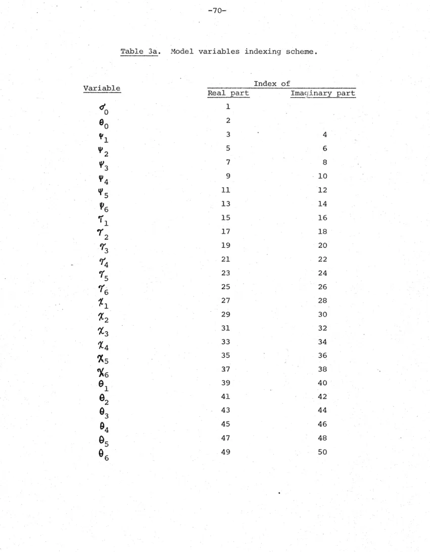
5. Model statistics . .... ... . . ... . 69 5a. Description of the statistical methods. .. .. . .. ... 72 5b. Invariance properties and the effect of

persistence on the number of independent observations . 77 5c. Reliability of the statistics ... . . .... . . . . . 78 5d. Statistical intercomparisons . ... .. ... 81 6. Model tuning . . . . . . . . . . . . . . . . . . .

6a. Tuning procedure. . . . . . . . . . . . . . .

6b. Tuning the QG model and results . . . . . . .

7. Monte Carlo simulation . . . . . . . . . . . . . .

7a. Analysis of the short term prediction errors. 7b. Adjustment to ccnserve energy invariants.

7c. Perturbing the QG model and results .. . .

8. Summary and concluding remarks . . . . . . . .

References . . .. . . . ... Acknowledgements . . . . . . . . . . . . . .... . . . . . .116 ... . . . 116 . . . . . .121 .127 .127 .133 .136 . . . . . . . 141 * . . . . .147 . . . . . . . 152 . . . . . . . . . . . . . 6 r, I - 'V'aL - - - - -- - -- ' -

-Figures

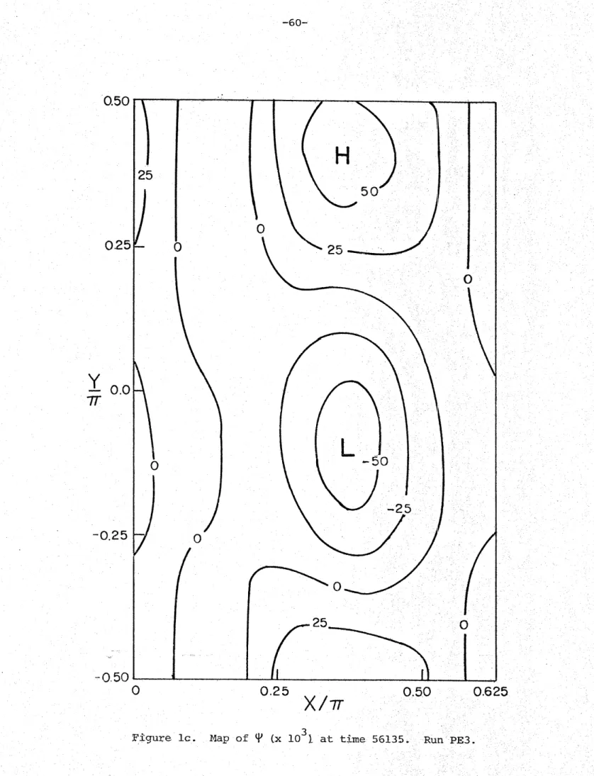
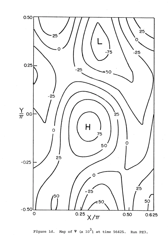
1. Typical maps of . . . . . . . . . . .

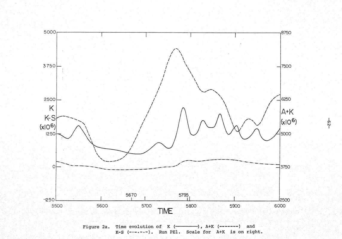
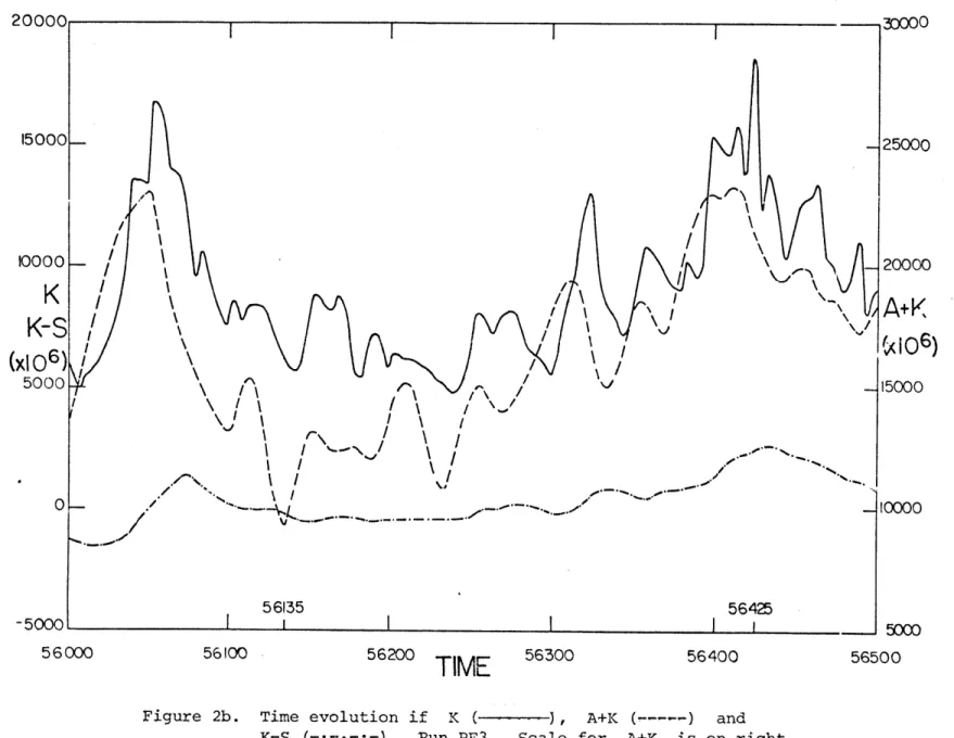
2. Typical evolutions of energy -ariables 3. Energy bu'dget of run PE3 decompos-E int-o

short and long time scales . . . . . . . .

4. Depiction of short term prediction error 5. Energy budget of PQG7. . . . . . . . . . .

Tables

1. Wave vector numbering scheme . . . . . . .

2. List of experiments. . . . . . . . . . . .

3. Variable indexing schemes . . . . . . .

2 2

4. Relative undertainty in 2 and 0 /

x x

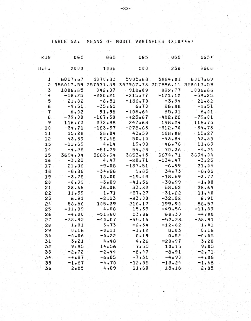
5. Effect of sampling and filtering on model

6. 7. 8. 9. 10. variable statistics. . . . . . . . . . . .

Intercomparison of model variable statistic Intercomparison of energy variable statisti Intercomparison of maintenance budgets . .

Tuning the QG model. . . . . . . . . . . .

Regression analysis results. . . . . . . .

Page . . . . . . . . . . 58-61 . . . . . . . . . . 62-63 . . . . . . . . . . 122 . . . . . . . . . . 139 . . . . . . . . . . 49 . . . . . . . . . . 54 . . . . . . . . . . 70-71 2 S. . . . . . . . 75 y . . . . . . . . . . 82-86 s . . . . . . . . . 87-94 cs. . ... ... . 95-100 . . . 108-111 . . . . . . . . . . 124 131 0

-4-ALTERATIONS OF THE CLIMATE OF A PRIMITIVE EQUATIONS MODEL PRODUCED BY FILTERING APPROXIMATIONS AND

SUBSEQUENT TUNING AND STOCHASTIC FORCI1G

by

ROSS N. HOFFMAN

Submitted to the Department of Meteorology in January 1980 in partial fulfillment of the requirements for the Degree of Doctor of Philosophy.

ABSTRACT

The simulated climates of nonlinear models based on the primitive equations (PE), balance equations (BE) and quasigeostrophic (QG)

equations are compared. The models and numerical procedures are iden-tical in all possible respects. 50 and 26 independen: functions of time alone represent respectively the solutions of the3 PE model and of the filtered models. The models are highly truncaj ed spectral forms of Lorenz's (1960) energy preserving two layer model. It is assumed that the domain of integration is a doubly pe:riodic f-plane, that static stability does not vary horizontally and that linear formulae govern vertical exchanges of heat and momentum. Because of the models' extreme simplicity very long time integrations (greater than 50 years in some cases) are easily effected.

Two levels of the thermal forcing are-considered corresponding to radiatively enforced pole to equator temperature contrasts of

100K and 400K. At low forcing (Ro -' 0.11) internal

gravity waves in the PE solutions are present only as initial transient disturbances. At high forcing (Ro Ad 0.33) internal gravity waves are always present in the PE solution. In the time mean sense the gravity waves obtain their energy from the synoptic scale waves and are frictionally dissipated

Transports are reasonably well simulated by the QG model at both forcing levels. At the low level of forcing the QG model and at the high level of forcing the BE model are successful at simulating the PE mean states and energy cycles. At high forcing the QG model gives only a qualitatively correct simulation of the'PE mean state and

energy cycle. The filtered equations always tend to underestimate the time mean gross static stability, energy flows and kinetic energy.

At the high level of forcing two attempts are made to get better simulations of the PE climate within the QG framework - the tuned and perturbed QG models. Both the tuning procedure and the perturbation procedure require some knowledge of the short term (5f-1 ,f = Coriolis parameter) _{prediction errors caused by the QG assumption. The QG model}

is tuned to minimize the av>ragc

o

ae c Jhort term prediction ero-,s. The tuned QG model is better than the untuned version at simulating the PE time mean model state, but the simulated energy cycle and the budgets maintaining the mean state are not improved at all. In the perturbed QG modeL randomly generated perturbations are added to the model state every 5f-1. These perturbations are designed so that their statistics, other than those involving time lags, are similar to the statistics of the observed prediction errors. The perturbations are adjusted to conserve the energy invariants of the system thereby ensuring bounded solutions. The perturbed QG model is nearly as success-ful as the BE model at simulating the PE climate.

Thesis Supervisor: Prof. E.N. Lorenz

-6-Preface.

The purpose of this preface is to provide background materiaL for those unfamiliar with the concepts discussed here and to provide orien-tation for assessing the value of the reported results.

Meteorology is based on the belief that the atmosphere uniformly obeys certain basic physical laws. These laws together with some

simplifying assumptions allow the deduction of mathematical equations which govern the time evolution of the atmosphere. If we know the exact equations, the exact composition of the atmosphere, the exact state of the boundaries of the atmosphere initially and for all future time and the exact current state of the atmosphere we would in principle be able to predict the evolution of the atmosphere for all future time. In fact our knowledge is an will always be far from exact - consider for example future readers of this page whose every breath must be involved in an exact formulation of the boundary conditions. As our knowledge is inexact our predictions will be inexact. It is expected that as we improve our knowledge (ard our numerical skill) our predictions will improve.

It is known that the atmosphere is unstable in the sense that small differences in the initial states generally result in larger differences

in the future states. Thalt is to say any errors introduced by our

approximations or inadequate observing procedures tend to grow with time. Eventually the true and forecast future states bear no resemblance to each other. Therefore there is a time beyond which our predictions are

worthless. However we cain still attempt to predict the future climate. We identify the climate with the long time period statistics of the

atmosphere. An example of great interest of the various atmospheric

statistics making up the climate is the time averaged pole to equator temperature gradient. This tem'perature gradient is maintained by three processes - solar heating, infrared cooling to space and the transport of heat by the atmosphere and oceans. Th1 differentially imposed heating drives the atmospheric motions. Besides affecting our comfort directly, the day to day weather transports heat poleward ensuring a relatively moderate pole to equator temperature gradient. If the trans-ports were temporarily suppressed the radiative effects would soon

strike a new balance with higher temperatures near the equator and cooler temperatures near the poles. Such a situation, while possible, would be unstable and atmospheric motions, which transport heat poleward, would soon develop.

Since the basic physical laws do not change it is a reasonable guess that the future and past statistics of the atmospjhere are identical. This hypothesis will be good to the extent that the boundary conditions and composition of the atmosphere do not vary and to the extent that the climate is independent of the initial state of the atmosphere. Climate theory attenipts to predict the atmospher:c statistics given the boundary conditions and composition of the atmosphere. If we specify the boundary conditions and composition of the atmosphere and assume that the initial conditions are not relevant then the problem as posed is exact except for our inexact knowledge of the governing equations. Besides being of theoretical interest, the answers to climate questions have important consequences for human existence. How would the climate change if the sun's output decreased slightly?

Would

an ice age ensue? Would an increase of atmospheric dust be equivalent to a slight decrease in the sun's output? Does overgrazing by cattle induce changes in

-8-&limate? Will the addition of carbon dioxide from burning coal or the adCition of flurocarbons from spray cans noticeably alter our cli-mate? These questions and others are under current study. Reliable

answers to thee rplestions will be necessary if society decides toqaintain or improve the quality of the environment. Meteorological studies of the

large scale circulation always suffer from an inability to perform real experiments. We are always forced to make do with models, which, no matter how complex, involve some degree of approximation. We must scru-tinize our approximations to establish the reliability of our answers.

The advances of modern meteorology are due in large part to syste-matic approximations based on the introduction of a priori estimates of the scales of the motions of interest. In particular, the theory known as quasigeostrophic (QG) scaling has helped explain the processes con-trolling the large scale atmospheric motions which influence the day to day weather we experience. Basically it is assumed that the time scale of the motions of interest is long compared to the time scales of the other motions. Let C represent the magnitude of the typical velocities of interest. In a midlatltude storm system C is roughly 50 km/hr.

Let L be a typical leng:h. The radius of a midlatitude storm might be 1000 km. During a period of time T , a particle embedded in the flow would move roughly a distance equal to C times T . If we choose a time period equal to L/C the distance traveled will be roughly L A particle in the center of our typical storm might travel to the edge of the storm in this length of time - approximately one day. This is

the time scale of the motions of interest. A coAvenient measure of this time scale is the Rossby number. The Rossby number (denoted Ro ) appears explicitly in the equations which govern all atmospheric motions

when these equations are put in a certain nondimensional form. (Nondimen-sional form is a standard form in which no references to units of mea-surement, such as meters, hours or degrees, are present.) The Rossby number is simply a constant (which depends on the latitude of interest) times the ratio of the time of the earth's rotation to the characteristic time scale. For our midlatitude storm the Rossby number is approximately one eighth. For motions which are characterized by faster speeds or shorter lengths the time scale is smaller and the Rossby number is larger. Two types of motions with small time scales present in the atmosphere are sound waves and gravity waves. (Ai example of gravity waves in a different setting is the ripples on the surface of a pond after a stone is tossed in.) By assuming at the start that the Rossby number is small the equations can be simplified. These simpler equations are called the filtered equations because they filter out the motions with small time scales. There are two commonly used sets of filtered equations, the QG equations and the balance equations (BE). The BE are more accurate and much more complicated mathematically than the QG equa-tions. The original equations, called the primitive equations (PE), are themselves inexact because a number of assumptions must be made in deriving them from :he physical laws. However for our purposes they may be considered exact.

The filtered equations have been the basis cf many studies of the large scale atmospheric motions. For qualitative understanding of the day to day weather the acoustic and gravity waves are extraneous. The filtered equations isolate the relevant motions.. By studying the QG equations we can understand the processes which control the motions and development of typical storm systems.

-10-The filtered equations are also routinely used fo- predictive pur-poses _{In numerical weather prediction (NWP) the future state of the} atmosphere is extrapolated from the observed state of the atmosphere according to the governing equations. To properly describe the motions the extrapolation takes place by a time marching procedure where the time step is smaller than the time scale of the motions. Thus a

smaller time step (and hence more computations) are required if the PE are used since short time scales may be present. If we use the PE it is also more difficult to initialize the time marching procedure because small errors in the observations can easily produce large gravity waves in the numerical solution which would not exist in the atmosphere. It was originally felt that the difficulties associated with the PE were

insurmountable and the first successful NWP was based on simpler govern-ing equations. While thE U.S. National Meteorological Center routinely integrates the PE, the meteorological services of several other nations use various forms of the filtered equations to produce their primary product.

We know that assumirg the filtering approximations are correct will introduce some errors over a prediction interval of a day or so but this is acceptable if there are other errors of similar or larger magni-tude caused by the uncertainty of the observations and by computational limitations. Thus a NWP model may be labeled "good" if it introduces a negligible error over the short time scale. Such a model may be inap-propriate for climate studies since these errors may accumulate and influence the model's statistics over the long time period needed to simulate the climate.

while many employ the QG assumption some of the more complex models are based on the PE. Because of the many differences between t'e various models and the atmosphere and between the models themselves it is diffi-cult to assess the effects of the QG assumption alone. Will the er. -rs introduced by the QG assumption over the short time scale tend to

accumulate or cancel out when we collect statistics? This question is addressed in the present study. We construct models which are completely identical in all respects but one - whether or not one of the filtering assumptions is made. Therefore any differences observed between the behaviors of the mod.els are due to the filtering assumptions. The models are integrated numerically and statistics are collected. For the sake of economy many similifications are incorporated in the models. This is acceptable since in any comparisons made, both mocels include the same simplifications. Fcr a low level of the thermal :orcing (i.e., the solar heating) the climates simulated by the QG and PE iodels are nearly

iden-tical. At a higher level of the thermal forcing -he different models generate quite diffierent climates; that is, the s'hort term errors tend to accumulate. For example, compared to the resul'ts of the PE model, the time averaged pole to equator temperature gradient of the QG model is

23% too low, while that of the BE model is 5% too low. However

quali-tatively the three simulated climates are very similar. Thus the appro-priateness of the filtering assumptions for climate studies depends on

the values of the external parameters. Generally the filtered equations are suitable for making qualitative climate predictions. The PE should be used whenever a quantitative result is required or when the quali-tative results of a filtered equations experiment are not decisive.

-12-It is conceivable that m,1ring slight changes to the QG model would improve its ability to simulate the DE model's climate. Most models of the atmosphere contain some adjustable parameters which owe their origin to the parameterization of subgrid scale pr-c-7 es or of physical pro-cesses not explicitly represented in the model. Tuning is the process of choosing values for these adjustable parameters. An example of an adjustable parameter is the drag coefficient C which appears in the

D

equation for horizontal stress / in the skin friction formula,

0CDI

CD

₀ u ₀

where

90

and O are the horizontal velocity and the density at some reference level. This formula is useful for representing the fric-tional drag of the earth's surface on the atmosphere. Actually the exchange of momentum between the surface and the atmosphere is mediated by molecular collisions so some simplification is necessary. It is possi-ble to obtain values of CD by measuring the other quantities in the above formula at a particular point and under particular conditions. Empirical values obtained in this manner vary considerably and it is not clear what the single best value is. Further, values valid at parti-cular points are not necessarily appropriate for diagnostic or predictive finite grid calculations. As pointed out by Lorenz (1951) the effects of small hills are not eplicitly present in any model but might be included in the calculations of 0 by choosing a slightly different

-0

value of C_D . In this study we consider whether or not tuning the parameters which appear in the QG model would improve its simulation of the PE climate at the high level of the thermal forcing. In some

respects tuning the QG model leads to an improved simulation. The time averaged pole to equator temperature gradient of the tuned t; model is found to be 7% higher than the PE value. Compared to the error of the original QG model the sign of the error is >eversed and the magnitud: of the error is considerably less.

Within the framework of a simplified model the short term errors caused by the simplifying assumptions are fundamentally unknowable. However by examining the assumptions it may be possible to estimate the magnitude of the errors. Suppose the statistics of the short term errors

are known. Can this knowledge be used to improve the model? Along similar lines, several techniques have been suggested for making use of the statistics of the errors in the initial conditions for predictive purposes. The most straightforward of these, Monte Carlo prediction, is

applicable to climate problems. In Monte Carlo prediction the observa-tions are assumed to be known to a certain accuracy and an ensemble

(i.e., a collection) of equally possible initial ;tates are chosen. From each of these initial states a prediction is made. The average of the ensemble of final states is generally a better fo iecast than a prediction made from just one initial state. Furthermore the variability within

the ensemble of final states gives an indication cf the reliability of the forecast. Part of this procedure was (and possibly is now) actually in operation at the New Zealand Meteorological Of1fice (Trenberth and Neale, 1977). Threa alternate forecasts were prcvided each based on a different analysis of the available data. (In this case, the initial

state is only poorly known since New Zealand is surrounded by water and weather ships are expensive to operate.) The difficulty here is that

-14-as are needed for a single forec-14-ast. Actually one would prefer an ensem-ble with more than three members. No extra computation is needed in Monte Carlo climate simulations because we can assume that the climate of each ensemble member is the same. In applying the method we add a small perturbation to the current state of the model after each short term time interval. These perturbations are random but have statistics similar to those of the short term errors. This method was tested on the QG model at the high level of the thermal forcing. The resulting climate agrees much better with that of the PE model. The pole to

equator temperature gradient is still in error - the sign of the error is reversed as in the case of the tuned model and the magnitude of the error is now 9%. However nearly perfect knowledge of the short term error statistics did not in this case lead to perfect agreement between the climates. It must be added that the QG statistics are constrained in a way that the PE statistics are not. Therefore perfect agreement is impossible unless the PE statistics satisfy these constraints.

The result that the perturbed QG model out performs the QG model is important because it runs counter to intuition. Offhand one would not expect that a model's response would be improved by adding a random

forcing. This technique suffers from one serious drawback - one must know the short term error statistics. Error statistics obtained from comparisons with observations would only be valid undei current climate conditions. This problem is left unanswered by the present study, but in cases where the error statistics are known this knowledge should be used.

~

1. Introduction.

When studying the climatte one is faced with the problem of describing the statistics of a system whose time evolution is essentially nonlinear and which is e-tremely sensitive to iritial conditions. A popular

plan of attack is to develop a numerical model, integrate it in time

and collect statistics. At each time step the current state of the model, which depends on the past history of the model, may be considered the initial conditions for the remainder of the model run. Thus any assump-tions introduced in deriving the model may be thought of as introducing errors into the initial conditions. As these errors compound their total effect may be large, although individual errors are small. It has been envisioned (Lorenz, 1970) that eventually super models may provide a solid basis for climate research. However any nurmerical model must involve some approximation and thus introduce some errors. Although the errors introduced by a particular assumption are unknowable within the context of the model some knowledge of the statistics of the errors may be obained by comparing short term predictions of the model to either a more complex model or the atmosphere itself. I: seems likely to the writer that such information, properly used, woull improve the fidelity of the model's simulation of the climate.

Beginning with Phillips (1956) increasingly complex numerical models have been developed for modeling the atmosphere over long time scales. Over time the model: have become better at simulating the atmosphere. However important differences exist between the observed climate and

the model climates. Even the most complex of the current models involve many assumptions, so it is difficult to determine which assumptions

-16-to compare the model output -16-to that of another model identic.l in all respects except that the assumption in question is relaxed. This

approach

is exemplified by the work of Manabe and coworkers at GFDL (Manabe et. al., 1970; Manabe and Terpstra, 1974; Manabe and Wetherald, 1975;

Wetherald and Manabe, 1975). Of course the effects of several assumptions are not necessarily additive so the appropriateness of any particular assumption depends upon the "environment" in which it is employed.

In this report we compare the simulated climates of nonlinear models based on the primitive equations (PE), balance equations (BE) and quasigeo-strophic (QG) equations. The models and numerical procedures are iden-tical in all possible respects. 50 and 26 independent functions of time alone represent respectively the solutions of the PE model and of the filtered (i.e., QG and BE) models. The models are highly truncated spectral forms of Lorenz' (1960) energy preserving two layer model. We assume that the domain of integration is a doubly periodic f-plane, that static stability does not vary horizontally and that linear formulae govern vertical exchanges of heat and momentum. Because of the models' extreme simplicity very long time integrations (greater than 50 years in some cases) are easily effected. Thus even small differences between the model climates may be determined with high statistical significance. Further, we investigate tvo means of making use of the information con-tained in the (presumed) hnown short term prediction error statistics. The first technique is to tune the adjustable parameters which appear in the model. The second technique is to add perturbationv to the model state at regular intervals; these perturbations have carefully designed statistical properties. (Reader beware! In this paper, excluding the portions reviewing previous studies, "perturbation" should connote

neither linearization nor infinitesimally small.)

The results of these experiments may be viewed from two perspectives. Fir3t, we may consider the PE model to be the "real" system we wish to

simulate. In this light the results are quantitatively correct and differences in (model) climates are due solely to the filtering assump-tions. Second, we may extrapolate our results to more complex models of the atmosphere. This is risky; the extrapolated results should be used only as suggestions of the qualitative nature of the errors caused by the filtering assumptions in more complex systems.

Although most suitable for short prediction intervals the QG assump-tion has proved extremely useful not only in nume.-ical weather predicassump-tion and linear stability studies but also in diagnostic and simulation

studies and in simple climate models. Surprisincly, until now no direct comparison of the climates of identical PE and QG models has been made. When a model is "improved" and the QG assumption is dropped it is gen-erally easier to reformulate the model from scratch. Then there is a tendency to go "whol..e hog", relaxing several other assumptions simul-taneously. The BE

have

seen limited use in numerical weather prediction. The long term behavior of BE models has been unknown because the BE are more difficult to integrate than the PE.

Quasigeostrophic theory has by now a long hi-tory and many authors have commented on the conditions necessary for its validity. Previous studies of the baroclinic instability problem rexcal the effects of the geostrophic assumption on the growth rates and structures of exponentially growing infinitesimal Rossby waves. Of the several studies noted here only one (Simmons and Hoskins, 1976) contains a direct comparison of a PE model and a QG model linearized about the same basic states. A point

-18-to keep in mind when comparing models differing in more tha. one respect is that it is difficult to assign portions of the error to the different assumptions. It is possible that several assumptions, each of which individually causes a significant error, may together cause only a small total error; the opposite situation of several assumptions each causing small errors which together cause an appreciable total error is also possible. As the principal interest here is in a comparison of nonlinear

systems we consider several topics which bear on the applicability of the results of linear theory under nonlinear conditions. Following this, we will review some nonlinear results.

Before reviewing the literature we define two terms. One approach to determine the adequacy of the QG assumption is to study data from actual observations or from a model which does not depend on the QG assumption. Differences from geostrophic balance in the data may then be attributed to effects not included in QG models. TIese differences may be termed ageostrophic. A second approach, the approach used here, is to compare two models, one of which employs the QG assumption. The total difference between the results of the two models may be partly in geostrophic balance. This total difference has been termed

non-quasigeostrophic (Gall, 1977). The first approach provides only a lower bound for the macnitudes of the errors caused by the QG assump-tion.

The baroclinic instability problem may be stated in brief, as fol-lows. The radiatively enforced or the observed zonally averaged pole to equator temperature gradient might be geostro hically balanced by a zonal thermal wind if the earth's surface were homogeneous and if fric-tional effects were absent. However, if the temperature gradient exceeds

a critical value such a basic state is baroclinically unstable; that is, small disturbances will grow by releasing some of the avaiL±ble potential energy of the basic state. Those instabilities with the fastest growth rates are seen to correspond in certain res,;ects to the observed di?-turbances. Although the observed atmospheric disturbances are far from infinitesimal in amplitude, the observed mid-latitude atmospheric structure is basically zonal with superposed perturbations. It is

argued that this zonally averaged state is always spawning growing baro-clinic disturbances whose growth is ultimately checked by dissipative processes or nonlinearities. As they extract energy from the mean flow these disturbances tend to decrease the pole to equator temperature gradient. This suggests the average state of the atmosphere should be close to neutral stability with respect to these

disturbances.

The evidence (Stone, 1978) in the extratropical regicrs supports this con-tention. For this reason and for analytic convenience many studies have focused on the neutral or nearly neutral case.

To the extent -hat other processes simply limit their amplitudes the calculated instabilities with the greatest growth rates are valid for parameterizing eddy fluxes for use in simple climate models. For this purpose it is still necessary to determine the amplitudes at which growth stops. Besides this closure problem there are two facts which make it difficult t- directly apply the results of baroclinic instability theory. First, the structure of the linear wave! and their growth rate spectrum - in particular the wavelength of maximum instability - depend very strongly on the presumed basic state and on-the numerical model.

-20-Not constrained by the feedbLaks present in a nonlinear system the linear results are very sensitive to modeling assumptions. Second, and partly as a consequence of the previous point, as the waves reach finite

amplitude interactions wich the mean flow profoundly affect both growth rates and structure. Therefore the concept of the "evolutionary"

selection of structures having the greatest linear growth rates must be abandoned or modified to include second order processes. Thus, if we wish to extrapolate comparisons of PE and QG linear instabilities

to the nonlinear regime we must choose the "right" basic state and include second order processes in some way. Simmons and Hoskins (1978) observed that in some cases the dependence on the presumed basic state becomes less marked when the wave is allowed to grow to finite amplitude and interact with the mean flow. An analogous result might hold for the dependence on the governirg equations. That is, it is possible that finite amplitude perturbations of PE and QG models allowing wave mean flow interactions are more alike in structure than the instabilities of the corresponding strictly linear models.

The earliest studies of baroclinic instability employed the geo-strophic approximation. (A succinct review is given by Phillips

(1963, Section 3a). A brief historical summary of the problem when geostrophy is assumed and when the zonal wind profile of the basic state is simple, is given by Geisler and Garcia in the introduction to their 1977 paper.) In fact the earliest formal quasigeostrophic scaling argument was motivated by the baroclinic instability problem

(Charney, 1947, 1948). Mcre recently the study of this problem has evolved along two paths. One approach is to make enough simplifying assumptions, usually including that of quasigeostrophy, so that analytic

solutions are obtained which explicitly display the dependence of the instabilities on the mean state variables (Saltzman and Tang, 1975; Stone, 1972; and references in these papers). When these results are incorporated into simple climate models the fluxes due to the mean meri-dional circulation forced by the waves should also be included (Stone, 1972). Along the second path of investigation several of the various assumptions made in the earliest studies have been relaxed and the numeri-cal numeri-calculations have increased in complexity. Derome and Dolph (1970) studied higher order effects on the disturbances and found slower growth rates and some differences in the structure of the disturbances. (Accord-ing to Mak (1978) Derome and Dolph were not careful enough in their

consideration of the boundary conditions - the problem they solved is ill-posed and their results are therefore questionable.) Hollingsworth

(1975) investigated the differences between the rormal modes of several variants of Lorenz': (1960) two layer model (the model used in the present study). On an f-plane channel Hollingsworth found the growth rate spectra of the short waves in the QG model are highly sersitive to whether or not the static stab lity is allowed to vary. Cortparing the results of the QG and BE models with variable static stabil ty he found similar growth rate spectra but indicated that substantial differences in struc-ture exist. On a sphere differences between the two QG models are less pronounced. Warn's (1976) calculated instabilities of two shallow layers on a sphere are sic ificantly ageostrophic. Simmrons and Hoskins (1976)

compared the normal modes of the PE and QG equations on a sphere for three simple zonal flows. In their study the models are identical except for the geostrophic assumption. The modes of the two models are similar;

-22-growth rates and relative anlitudes agree to OCRo) . However agree-ment in terms second order in amp±ltude is poorer - when normalized to

a constant value of maximum perturbatic.n stream function the eddy meri-dional fluxes of heat and zonal momentum differ by as much as 25% and 50% respectively. Also the neglect of vertical transports in the QG model leads to poor agreement of the second order changes to the mean state. Gall (1977) calculated the normal modes of an f-plane channel with an idealized zonal flow symmetric about mid-channel. For this geometry and basic state the QG perturbation equations decouple into symmetric and antisymmetric components. Gall used symmetric initial conditions. Therefore any asymmetries which developed in the solutions of the

linearized PE must be die to non-quasigeostrophic effects. (This proce-dure will not detect non-quasigeostrophic effects on the symmetric part of the perturbation.) Gall found that the perturbation fields and meri-dional heat transports are fairly symmetric but the merimeri-dional fluxes of geopotential and zonal momentum are noticeably antisymmetric. As noted by Gall, these results are not surprising as these latter fluxes are

covariances of perturbation quantities which are roughly 90" out of phase. Points relevant to the application of these compa:.isons to the

nonlinear regime are made in several related studies cf FE models b Simmons and Hoskins and by Gall and his coworkers. There is some controversy over the wavelength of maximum growth rate in the linear models. Gall (1976a, 1976b, 1976c) found a maximum growth rate for wave numbers 12 through 15 while Simmons and Hoskins (1976, 1977a) found a maximum growth rate for wave number 5 through 9. Some of the difference is due to the assumed basic state (Simmons and Hoskins, 1977b; Gall and Blakeslee, 1977;

Staley and Gall, 1977) but the issue is not resolved. It is possible that

details of the model may be crucial. If this is so, application of the linear results to other models or to the atmosphere must be questioned. At

any

rate, linear growth rate spectra are very sensitive to the basic state. Since the basic state of a nonlinear model or of the atmosphere is constantly changing it is not clear how to apply the linear results. A partial explanation of the sensitive dependence of growth rate spectra on the basic state was noted by Fullmer (1979), using a one dimensional QG model. He found that small changes in the basic state zonal wind can lead to very different growth rate spectra if these small changes in the zonal wind are associated with relatively large changes in the mean profile of the QG potential vorticity gradient, which is the quantity

appearing in the stability criterion. In their experiments Simmons and Hoskins found that the meridional flux of zonal n.omentum is sensitive to the assumed basi; state while the meridional Ieat flux is relatively insensitive.

Most of the calculated normal modes have maximum amplitude near the surface; the shorter the wavelength the more the mode is restricted to lower levels. A3 a consequence most of the fluxes due to the linear waves are restricte1, to the surface layer. Gall (1976a) compared the normal modes of the GFDL global circulation model (GCM) to both obser-vational statistics and statistics obtained from The GCM. In contrast to the linear case the most energetic wave numbers in the GCM and in the observations ar. those less than 9 and these eddies have maximum amplitudes of kinetic energy and momentum transport in the upper

troposphere. By allowing growth to finite amplitude and wave mean flow interactions both Gall (1976b) and Simmons and Hoskins (1978) found

-24-the growth of maximum amplitude at upper levels, -24-thereby favoring -24-the select-.on of longer wavelengths. In contrast, Sinmons (1972), who studied the same problem with a QG model, reported that the finite amplitude wave kinetic energy profiles agreed with those of linear waves.

In summary, baroclinic instability results indicate significant differences between PE and QG linear waves. In particular relatively minor structural differences can result in much larger differences in eddy fluxes. Also indicated is the importance of wave mean flow inter-actions when the waves reach finite amplitude. The effects of the wave mean flow interactions seem to be as or more important than differences between the PE and QG linear waves. Therefore if a linear theory is acceptable,. the errors introduced by the additional assumption of quasi-geostrophy are acceptable. On the other hand it is questionable whether we can extrapolate the comparison of PE and QG linear waves to a non-linear regime.

Heck (1979) calculated the eddy flux of zonal momentum directly from observational data and diagnostically as a residual of the potential

temperature and potential vorticity fluxes. If the atmosphere were quasigeostrophic the two calculations should agree. Heck found that the QG assumption causes a relative error of 25% to 60% depending on latitude and season. This is the same order of magnitude as the linear results of Simmons and Hoskins (1976). But it should he noted that they calculated non-quasigeostrophic differences and Heck c.lculated ageo-strophic differences.

Semtner and Holland (1978) compared several QG models with a PE model. Their study shares this objective with the present study but there are major differences in the physical situations considered and in

the models used. Semtner and Holland model a primarily wind driven w- stern North Atlantic circulation using QG models having two or three layers and constant mean stability and a PE model having five layers. The QG mode~' and PE model differ in the details of bottom tp -nraphy, friction, heating and in other respects. In all, eight QG experiments were performed, demonstrating, among other results, the necessity of including at least simple topography and heating in the QG model to properly simulate the PE model's climate. Semtner and Holland origi-nally felt that the basic QG experiment which includes topography and heating would simulate the PE results best. Qualitatively good agreement is obtained but the eddies in the QG model are too intense; the QG

energy levels are approximately 35% higher than thie PE energy levels and the QG kinetic energy conversion is too high. Sentner and Holland then tuned the QG model ]by changing the upper layer thickness from 500m to

200m. This results in good agreement with the PE results. Thus the QG equations are sensitive to vertical discretization. (See also Flierl

(1978).) However it is not obvious how good the agreement would be between a QG model ind a PE model with identical vertical structure.

Inevitably, as noted earlier, in any numerical model small errors occur at each time ;step; these errors may amplify, limiting the usefulness of the model for simulation purposes. It seems a reasonable hypothesis that anything decreasing the magnitude of the shcrt term prediction

errors will improvE the model's ability to simulate the observed climate. A number of empirical methods for decreasing the magnitude of the pre-diction errors have been proposed - model tuning, the empirical correction method and the empirical dynamical method. (See Leith (1978a) for a

-26-of the real system. _{(This limitation is discussed in the co'clusion.)} Although most models have some adjustable coefficients, tunil-rT is nearly a taboo subject in the meteorological literature. From the discussions which do appear in the literature it appears that tuning is accomplished by rough qualitative argument followed by numerical experi-mentation. The tuning problem may however by put in the form of an

inverse problem if the condition of optimality can be mathematically defined. The single example of this approach we know of for a dynamical

system is given by Leith (1974b). Leith chooses , a parameter in the long wave correction of a barotropic model by plotting the ensemble averaged root mean square height error of the two day forecasts versus

X

and choosing the value of

2

corresponding to the minimum error. In geophysical diagnostic studies the inverse problem apiproach is more popular; for example Olbers et. al. (1976) determined wave spectra from moored array data using inverse techniques.

In Section 6 the QG model is tuned using data obtained from a PE model run to minimize the mean squared short term (5f

-) prediction error. In some respects the tuned quasigeostrophic (TQG) model is better able than the untuned model to simulate the PE model's climate.

In Leith's (1974b, 1978a) empirical or climate drift correction method the model equations are altered by adding constant and linear terms to the governing equlations. These new terms are statistically determined by requiring that the ensemble mean first and second order statistics are preserved. The tuning procedure is equivalent to an empirical correction method where a special form'of the corrections is assumed at the start of the analysis if the terms in the governing

equations containing the adjustable. parameters are coi.stant or linear (in the parameters). Faller and coworkers (Faller and Lee, 1975; Faller and Schemm, 1977; Schemm and Faller, 1977) proposed a statistical cor-rection method whereby an empirically determined corcor-rection is addc:& to the solution after each time step; they found significantly improved forecasts in experiments with one and two dimensional forms of a modi-fied Burger's equation. Their technique may be considered a finite difference approximation of Leith's empirical correction method.

Presently empirical climate models obtained by inverse techniques are receiving attention from Hasselmann and his coworkers, as outlined by Hasselmann in a

series

of lectures delivered at Harvard this spring.

(A number of papers are in preparation.) For climate simulation purposes Hasselman suggests seeking agreement between the model and the data in the frequency domain. A technique for accomplishing this was successfully tested by Hartjenstein and Egger (1979) using data from simple two

layer model experiments. They sought a constant coefficient linear

zonally averaged model which would simulate the u:onally averaged behavior of the original model. The model coefficients wEre found by demanding agreement between the low order Fourier coefficients of the original data and of the solutions generated by the linear model.

The empirical dynamical method uses the results of integrating a dynamical model as predictors of the forecast quantities in an empirical linear (in all stucies to date) regression schema based on observations. This method has been used in creating MOS forecasts (Klein and Glahn, 1974), in studies of a hemispheric barotropic model (Leith, 1974b; Lorenz, 1977) and in the final step of a Monte Carlo prediction study

-28-(Leith, 1974a).

It is not expected that the us of empirical methods will yield a perfect prediction model. Generally a substantial part of the mean

squared error remains. The residuals, i.e., Ch- differences between

the observed prediction errors and the empirical estimates of the predic-tion errors, may contain important informapredic-tion. We conjecture that the regular addition to the model state of random perturbations with theore-tically or empirically determined statistical properties may improve the model's ability to simulate reality. (In this study the observational

data are actually generated by a model, but for the purpose of discussion we will refer to this more complex model as "the real system"; the simpler model involving the additional assumption(s) will be called "the model".)

To illustrate this hypothesis assume that the real system's time evolution may be described by a point moving through a multi-dimensional phase space and that the model's time evolution is described by a point moving on a lower dimensional manifold in the real system's phase space. For predictive purposes we need an initialization procedure; this may be thought of as the projection of the system state on the model manifold. Now consider a point X(O) on the model manifold and the set X

of all points in the phase space which project onto X(0) and which are in the attractor set of the real system. Then the projection of the sys-tem state will come arbitrarily close to X(O) as often as desired over a long enough period of :ime, provided that the set Xj is not empty. After a short time T the model state will be X(T) and the points

i f

X _n will evolve to the points X . Generally the projection of the n

set X will not be a single point and the average of the projections

J

of the X will be dif1erent from X(T) . The statistics of the errors, n

where the errors are the difterences of the projections of Xf and n

X(T) , may be determined empirically or by theoretical consideration of the short term behavior of the sys m. r'he actual errors are of course unknowable within the context of the model. If the model is to give a good simulation of the system the point X(O) should be in the attractor set of the model. Suppose this is so; then the model state will come arbitrarily close to X(0) as often as desired for a long enough simulation. As the real system evolves every time its projection comes close to X(O) there will be a certain probability that the real system is close to a particular X . After a time T the projection

n

of the real system will be close to the projection of the corresponding f

X with the same probability. The unperturbed model evolution on the

n

other hand is completely determined. by X(0O) . The real system's behavior can be simulated by adding random perturbations to the model state

X(T) , if the statistical properties of the perturbations are chosen to agree with the statistical properties of the errors. This argument moti-vates but certainly does not prove our conjecturE

In Section 7 we test our conjecture by perturbing the QG model at regular intervals. The perturbations contain a deterministic component corresponding to a least squares estimate of the prediction error, that is an empirical coriection, and a stochastic component having statistical properties similar to those of the residuals of the least squares esti-mates of the prediction errors.

The addition of randomly generated perturbations to the model state at regular intervals is a finite difference form of adding stochastic forcing to the governing equations. In meteorolegy, stochastic forcing

-30-has been used previously in stoc-30-hastic prediction and in linear and non-linear climate modeling.

Since the beginning of modern numerical weather prediction there has been an awareness that predictability is limited by both the uncertainty in the initial conditions and shortcomings in the model (Thompson, 1957). Predictability studies have shown that even with.a perfect model the uncertainty in the initial conditions limits the useful forecast range to at most two weeks. Stochastic dynamic prediction has been proposed as an objective way of utilizing our knowledge of the uncertainty in the initial conditions. _{(Review papers by Leith (.1975) and Haltiner and} Williams (1975) cover both these topics.) Within the framework of sto-chastic dynamical prediction it is possible to include stosto-chastic forcing to take into account the effects of model insufficiencies on the forecast

(Fleming, 1972; Pitcher, 1.977). Because of the nonlinearity of the governing equations most stochastic dynamical prediction models rely on some sort of closure scheme for the higher statistical moments. Leith

(1974a) has suggested Monte Carlo methods may be more economical. Besides sidestepping the closure problem Monte Carlo predictior schemes should make it easier to include stochastic forcing.

Recently stochastic climate models have recieved considerable atten-tion. Hasselmann (1976) suggests that the effect of the short time scale weather phenomena on the long time scale climate system is essentially

that of white noise forcing. If a linearized model is adequate it is then possible to evaluate the climate system's frequency response for any given forcing by the weather. This technique has been successfully applied to the forcing by the atmosphere of observed sea surface tempera-ture anomalies (Frankignoul and Hasselmann, 1977; Reynolds, 1978) and of

a 8-plane ocean (Frankignoul and Muller, 1979) and to the parameteri-zation of atmospheric eddy heat fluxes in zonally and globally averaged energy climate models (Lemke (1977) and Fraedrich (1978) respectively). The effects of stochastic forcing on nonlinear (climate) models can in general only be evaluated by numerical means. Robock (1978) included a stochastically forced component in the parameterization of the zonally averaged poleward heat flux in Seller's (1973) time dependent model. The time evolution of the model's annually and globally averaged tempera-ture qualitatively agrees with observations. Williams (1978) incorporated a stochastic energy source in his barotropic model of the Jovian atmosphere, and found the model simulated flow is similar to observations. Without the stochastic forcing both of these models would asymptotically approach a steady or periodic solution for any initial conAitions. The present

study contains the

first

report of the response of an aperiodic climate model to stochastic forcing.

-32-?. The model.

2a. Coverning equations.

The model presented below is a spectral form of the energy pre-serving two lacyr model formulated by Lorenz (1960). For horizontally continuous variables the adiabatic, inviscid governing equations of this model are

?'el-J<ve~-JccT)

el -Crv

1

SP+

_ve'

₊

-F

+

V

.

ce

-

+

711i)

-SP

(vIZv'vT

+ -

Viv

t)

where

$

+ 0 is the potential temperature in the upper layer,

8

- g- is the potential temperature in the lower layer,

+

'

is the stream function in the upper layer,

-

7

is the sLream function in the lower layer,

f is the Coriolis parameter,

C is the specific heat of air at constant pressure, and P

b is a constant approximately equal to 0.124. J is the Jacobian operator defined by

J(A,B) = VA'(7B x k)

where k is the vertical unit vector and

V

is the horizontal gradient operator. There are two indi-cator variables distinguishing the three systems of equations.

0 for the QG equations and BE

1 for the PE

0 for the QG equations B 1 for the BE and PE

For a domain without horizontal boundaries, these equations possess three independent integral invariants which may be taken to be A+K , P+I+K and S-K. P+I , A , K and S are respectively the total potential energy, tiie available potential energy, the kinetic energy

and the gross static stability all averaged over the mass of the atmosphere. If the further simplifying assumptions that f is constant and that

0

does not vary h)rizontally, and if rectangular coordinates (x,y) and the scaling f-x, y L ,.:f x,y:L I $ : L2 f S- : L2 2 (C b)-1

-34-citez~=

TOV),%ay

.

2

_z(7Yv

₀₇

Olt

(VZT1

₊

_7XVvT)

V

2

_T

+5

P

( ,

v,7

2

x

,

- J(UVV7T)

0-t

P de

-

:T (T

,

7

+

V%

- 5

((VPi

7. -

,

(f

(7~zr('

v~r-TVY)

-

LV)JI

4r

y(%vZ')

e 0

=

0

where the overbar and q, and

90

represent areal averages and all other variables are deviations from areal averages. With this scaling there are no dimensionless constants in the equations of motion.

An infinite doubly periodic f-plane is chosen as the horizontal domain. Each of

e,

(,

7

and

/

is expanded in a complex Fourier series of the form

(1)

I(x,y,t) =

where the sum is over all integer wave vectors I = (Ix ,Iy), excluding

I = 0 and where I is an ordering of the I . (That is, the I(th) wave vector is I , the J(th) wave vector is J , etc.) In order that

g

be real I', where -I is the index of -I , must be equal to the complex conjugate of I for all I and for all .

F = exp(i(I x+I y))

I x y Consequently FF 0 if I+J 0 1 if +J ₌ 0 and

72F

= (-a )F I I I 2

where a = I*I is positive. Now substitute expressions like (1) into I

the nondimensional governing equations, multiply by F and average -I

horizontally. For linear terms

=

F F

A

J

-36-The quadratic terms all satisfy

F ,Q ( 3 )

F_IQ Fj f J FK ;K)

J K

Z= J IJK 'K

J K

where the interaction coefficients

qIJK = FIQ (F FK IJK -I J' K

are constants. The one term requiring special attention is

Tha adiahatic inviscid nondimensional equations of motion in spectral form are thus

T

C-1 7 K K4 +

o

O

(-

a

(2. a)L)

(2.a) d

- 2 _{Y - Ca.K (-Q. IV, YCI.}

&

_%

7

1

0,

_e

_/

₂₎

-a IA J

8 _{1 4 + - ,}

+ P

XT

:-(

C

K')%IC

&c f _{4-913. Cix 11( TIC} I 4z) I - 3- -Qz'Y +b Z( a, WK a., 0 where we have are written for 3 h

. The interaction coefficients

CIJK dIJK e IJK = _I J J(F , FK ) -I J K -= I V (Fj FK) -I FJ K - F- VFj- VF = F F *V'K where b = FF IJK -I J K (K x J)b IJK 2 2 2 = -(I + K - J )b - - IJK (2 2 2 = ( + K - I )b . - - IJK 1 if J + K= I 0 otherwise

These equations conserve the three energy invariaits of the original two layer equations. The only requirements for this to hold are that

S,

'P

,

7

and , are all expressed in terms of the same expansion

functions, and that whenever a wave voctor I is included in the expansion

C

x -,L~

rT+d o

-38-so is -I.

Diabatic and viscous processes must now be specified. Of the many possible parameterizations we choose the simplest. Since the principal interest here is in the differences between two systems of equations having identically parameterized friction and heating it is not expected that these differences will be overly influenced by the choice of para-meterizations. Second, simplicity is in keeping with the anticipated

severe truncation. Following the approach used by Lorenz (1962, 1963b) in studying QG models, we add to the model surface friction proportional to the velocity in the lower layer, a momentum exchange between the layers proportional to the velocity difference between the layers, a heat

exchange between the layers proportional to the piotential temperature difference between the layers, heating of the lower layer proportional to the difference between the temperature in the lower layer and an imposed temperature field and heating of the upper layer proportional to the difference between the temperature of the upper layer and an imposed temperature field. These last two effects may be thought of as due to radiative heating and/or boundary layer heating. If the propor-tionality constants, assumed all non-negative, are respectively 2fk₀,

f(k

₁ -k0L, fh ₀ , f(nl+h_{1 2} 2 ) and fhl -h 1 then the scaled spectral equations

1 2 (2.a). include the additional terms

(2.b)-

%

-(2.b) - ***''y &&2: - _i

%

=

..- h A _ _o 2 -

-A

eQo

_(OC

CR0

0~f

,

(+-lxL)Tr

k

o

-<r%

- h, %-ob~

o

,

(O-

b' - 0 + 0

'00-where the superscript R refers to the imposed (radiative) temperature field. The sketch on the next page illustrates the model physics.

2b. Energy equations.

The flow of energy through the system is governed by the usual energy equations, d -A dt d -K dt d -A dt Az d -A dt AE d -K dt KZ d = G - C = C - D G'_z = GE + = C -= C + E C - C A Z C - C C - D C - D K E

where A, K, G, C and D ;:epresent respectively the available form, kinetic form, generation, conversion and digsipation of energy averaged over the mass of the atmosphere. The subscripts Z, E, A and K denote

p=0 level 3: V3,3 -

8

3I p=p /2_l level 1: V, 1 P=P0 Momentum Exchange 1I --f(k -k ) (V -V 2 1 0 3 1 1 - -f(kl-k _{) (V -V} 2 1 0 -13 Heating -f(h l -h 2) (3- R) - fh0 (9B - ) Heat 0. 3 1 Exchange 1 2 0 f 1 3 R Heating -f(h ₁ +h2) ₂ O ?- _{1 1} ) Surface Friction -2fk V Surface Friction 0~1

Model physics in dimensional form.

____ __1 1_ ___

£espectively zonal, eddy, available and kinetic forms of energy or energy flow. The division into eddy and zonal forms is in the space domain

(Oort, 1964). Below the diagnostic equations for the energy variables are presented i,. trms of the nondimensional horizontally continue: -variables. (The scale for energies is L2f2.) The notation is more concise and it is easier to follow the derivation in this form; however exactly analogous statements may be made directly in terms of the spectral variables. For example, in terms of the continuous variables the hori-zontal average of any Jacobian term is zero because of the periodic boundary conditions while in terms of the spectral variables this holds because of the symmetry properties of the interaction coefficients;

c JK = -c-J,-IK = -c KJ All calculations reported in the sequel are

performed in the spectral domain.

The forms of energy for the two layer model (Lorelnz, 1960) are kine-tic energy, available energy, gross stakine-tic stability and total potential energy, which are defined respectively by

A

C.

-6

0.