How sensitive are optimal fully renewable power systems to technology cost uncertainty?

HAL Id: hal-02180343

https://hal.archives-ouvertes.fr/hal-02180343

Preprint submitted on 12 Jul 2019

HAL is a multi-disciplinary open access archive for the deposit and dissemination of sci-entific research documents, whether they are pub-lished or not. The documents may come from teaching and research institutions in France or abroad, or from public or private research centers.

L’archive ouverte pluridisciplinaire HAL, est destinée au dépôt et à la diffusion de documents scientifiques de niveau recherche, publiés ou non, émanant des établissements d’enseignement et de recherche français ou étrangers, des laboratoires publics ou privés.

How sensitive are optimal fully renewable power systems

to technology cost uncertainty?

Behrang Shirizadeh, Quentin Perrier, Philippe Qurion

To cite this version:

Behrang Shirizadeh, Quentin Perrier, Philippe Qurion. How sensitive are optimal fully renewable power systems to technology cost uncertainty?. 2019. �hal-02180343�

Behrang Shirizadeh

Quentin Perrier

Philippe Qurion

CIRED Working Paper

N° 2019-73 - Juillet 2019

How sensitive are optimal fully

renewable power systems

to technology cost uncertainty?

Contact : shirizadeh@centre-cired.fr

Jardin Tropical de Paris -- 45bis, avenue de la Belle Gabrielle 94736 Nogent-sur-Marne Cedex Site web: www.centre-cired.fr Twitter: @cired8568

Centre international de recherche sur l’environnement et le développement

1

Abstract

Many studies have demonstrated the feasibility of fully renewable power systems in various countries and regions. Yet the future costs of key technologies are highly uncertain and little is known about the robustness of a renewable power system to these uncertainties. To analyze it, we build 315 long-term cost scenarios on the basis of recent prospective studies, varying the costs of key technologies, and we model the optimal renewable power system for France over 18 meteorological years, simultaneously optimizing investment and dispatch.

Our results show that the total cost of a 100% system is not that sensitive to the power mix chosen in 2050. Certainly, the optimal energy mix is highly sensitive to cost assumptions: the installed capacity in PV, onshore wind and power-to-gas varies by a factor of 5, batteries and offshore wind even more. But the total cost will not be higher than today, and choosing a non-optimal electrical mix does not significantly increase this total cost. Contrary to current estimates of integration costs, this indicates that renewable technologies will become by and large substitutable.

Keywords: Power system modelling; Variable renewables; Electricity storage; Robust decision making.

2

Table of Contents

1

Introduction ... 4

2

Materials and methods ... 5

2.1 Model description ... 5 2.2 Model equations ... 8 Objective Function ... 8 Adequacy equation ... 8 Renewable power production ... 8 Energy storage ... 9 Secondary reserve requirement ... 9 Power-production-related constraints ... 10 Storage-related constraints ... 11 2.3 Input data ... 12 Cost data ... 12 VRE profiles ... 14 Electricity demand profile ... 14 Discount rate ... 14

3

Results ... 15

3.1 The optimal power mix is highly sensitive to power cost assumptions ... 15 3.2 However, setting a capacity mix in advance hardly increases costs ... 18 3.3 Sensitivity to weather data ... 19 Testing weather sensitivity ... 19

3 Selecting a representative year ... 21

4

Discussion & Conclusion ... 23

4.1 Comparison with existing studies ... 23 4.2 Model limitations ... 24 Factors which could push costs up ... 24 Factors which could bring costs down ... 25 4.3 Conclusion ... 26 References ... 28

Appendix 1. Additional information on the JRC 2017 study ... 32

Appendix 2. Wind and solar production profiles ... 34

Appendix 3. Weather year sensitivity ... 35

Appendix 4: the EOLES model ... 38

Appendix 5: Transport cost of carbon dioxide for methanation ... 41

Appendix 6: Cost decomposition ... 42

Appendix 7: Additional information ... 43

4

1 Introduction

1

According to Article 4.1 of the Paris Agreement, the Parties shall endeavor to rapidly reduce greenhouse gas emissions in order to achieve a balance between anthropogenic emissions by sources and removals by sinks in the second half of this century. From this point of view, the electricity sector will have a key role to play, as decarbonisation is considered to be easier in this sector than in transport, buildings or agriculture. Renewable energy will be the cornerstone of decarbonisation, making, with CO2 capture and storage, a greater contribution than nuclear energy and fossil fuels (Rogelj et al., 2018).

Following Joskow (2011) and Hirth (2015), many articles have focused on the optimal proportion of renewable energies in the electricity mix. This literature has highlighted the existence of systemic integration costs related to the deployment of variable renewable energies. In particular, a “self-cannibalization” phenomenon was highlighted, linked to the fact that all the solar panels in a given farm produce their electricity at the same time, just like wind turbines. In the absence of affordable storage, these integration costs have two consequences: (i) deployment of renewable energies leads to a significant additional cost, rapidly increasing with the deployment rate; (ii) the right balance must be struck between the different production technologies to minimize this additional cost. These results have direct policy implications in the trade-off between visibility and flexibility. On the one hand, investors want visibility for the development of economic sectors, such as quantified targets in terms of installed renewable capacity. On the other hand, a high sensitivity of the optimal power mix to technology costs argues for a flexible approach, allowing trajectories to be readjusted according to the evolution of technologies. Current results thus tend to support the flexibility approach – at the expense of visibility for investors.

However, these results of increasing costs and right balance might not hold much longer, due to the rapid decline in production and storage costs. In the space of seven years, the cost of solar panels has been reduced by a factor of seven, while batteries now seem to be following a similar pattern (Henze, 2019). Moreover, recent wind turbines benefit from a flatter production profile than older models (Hirth and Müller, 2016). Finally, methanation, which offers an alternative for seasonal storage, is also making significant progress. These developments will probably still be significant by 2050, the political horizon used today in the design of public policies. While the feasibility of a 100% renewable mix has already been highlighted by many studies (Brown et al, 2018, and references therein), the question is now that of cost sensitivity: do these reductions in production and storage costs call into question the previous conclusions about the announced high additional systemic cost of renewable energy?

5

If this phenomenon of increasing costs does not hold any more, it would mean that the relationship between renewable energy sources is changing from being complements to being substitutes. It would be then possible to identify one or several “robust” energy mixes, in the sense that their overall cost does not vary much, even if the cost of the different technologies finally differs from the initial forecasts. In such a case, the political conclusion would shift: proving flexibility to investors through fixed renewable targets would prevail over flexible approaches.

To shed light on these questions, we build a new open-source model called EOLES (Energy Optimization for Low Emission Systems) and apply it to continental France. EOLES minimizes the total system cost while satisfying power demand at each hour for a period of up to 18 years. It includes six power generation technologies (offshore and onshore wind, solar, two types of hydro and biogas) and three storage technologies (batteries, pumped hydro and power-to-gas). Using this model, we study the sensitivity of the power mix in 2050, through 315 cost scenarios for 2050, varying all key technology costs: onshore and offshore wind by +/- 25%; PV, batteries and power-to-gas by +/-50%. Then we aim to identify whether a robust power mix can be found. The remainder of this paper is organized as follows. In Section 2 we present the EOLES model. Results are presented in Section 3 while Section 4 provides a discussion and concludes.

2 Materials and methods

2.1 Model description

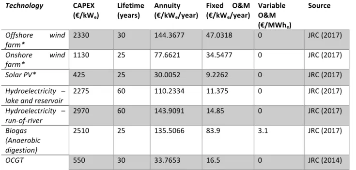
EOLES is a dispatch and investment model that carries out linear optimization with respect to total cost. It minimizes the annualized power generation and storage costs, including the cost of connection to the grid. The EOLES model includes six power generation technologies: offshore and onshore wind power, solar photovoltaics (PV), run-of-river and lake-generated hydro-electricity, and biogas combined with open-cycle gas turbines. It also includes three energy storage technologies: pump-hydro storage (PHS), batteries and methanation combined with open-cycle gas turbines. These technologies are shown in Figure 1.

The model considers continental France as a single node. PV and onshore wind are simulated for the 95 departments (an administrative entity corresponding to the European NUTS 3 level). The proportion of the installed capacity in each department remains the same in all simulations, at the level observed in

6 2017. The model is written in GAMS and solved using the CPLEX solver. The code and data are available on Github.1 Figure 2 provides an illustrative output of the model , i.e. the optimal dispatch for a week in winter and for a week in summer, as well as the corresponding power price, for each hour of the week.

The remainder of this section presents the main equations (2.2) and the input data (2.3). A detailed description of all sets, parameters and variables of the model is available in Appendix 4.

Figure 1 Graphical description of the EOLES model

7 Figure 2 Hourly power generation, electricity demand, storage charge and discharge profiles and power prices for (a) the third week of January (Winter) and (b) the third week of July (Summer) 2006

8

2.2 Model equations

Objective Function In EOLES, dispatch and investment are determined simultaneously by linear optimization. CAPEX (capital expenditure) and OPEX (operational expenditure). The objective function, shown in Equation (1), is the sum of all costs over the chosen period, including fixed investment costs, fixed O&M costs (which are both annualized) and variable costs. For some storage options, in addition to the CAPEX related to charging capacity per !"#, another type of CAPEX is introduced: a capex related to energy capacity, per !"ℎ#

%&'( = +#, *+#,− .+#,#/ ×1223456+#, + ?+@(:&;<=>?+@×1223456?+@#A) + +#,(*+#,×

C&&=+#,) + ?+@('?+@× E1FGHI5JEℎ

+

C&&=EℎI5J

)

+#, M(K+#,,M× N&&=+#,) /1000 (1) where *+#, represents the installed capacities of production, :&;<=>?+@ is the volume of energy

storage in MWh, '?+@

is the capacity of storage in MW, 1223456 is the annualized investment cost,

C&&= and N&&= respectively represents fixed and variable operation and maintenance costs and K_+#,,M is the hourly generation of each technology.

Adequacy equation

Electricity demand must be met for each hour. If power production exceeds electricity demand, the excess electricity can be either sent to storage units or curtailed (equation 3).

K_+#,,M

+#, ≥ SGT12SM+ ?+@'(&UVK>?+@,M (3)

Where K+#,,M is the power produced by technology tec at hour h and '(&UVK>?+@,M is the energy

entering the storage technology str at hour h.

Renewable power production

For each variable renewable energy (VRE) technology, the hourly power production is given by the hourly capacity factor profile multiplied by the installed capacity available for each hour (equation 4).

K_W@#,M= *_W@#× EC_W@#,M (4)

Where KW@#,M is the electricity produced by each VRE resource at hour h, *W@# is the installed capacity

9

Energy storage

Energy stored by storage option str at hour h+1 is equal to the energy stored at hour h plus the difference between the energy entering and leaving the storage option at hour h, accounting for charging and discharging efficiencies (equation 5):

'(&U>X_?+@,MYZ= '(&U>X_?+@,M+ ('(&UVK>_?+@,M×[_?+@\A _{) − (}]^_`,a

b^_`cd_) (5)

Where '(&U>X?+@,M is the energy in storage option str at hour h, while [?+@\A and [?+@ef+ are the charging

and discharging efficiencies.

Secondary reserve requirement

Three types of operating reserves are defined by ENTSO-E (2013), according to their activation speed. The fastest reserves are Frequency Containment Reserves (FCRs), which must be able to be on-line within 30 seconds. The second group is made up of Frequency Restoration Reserves (FRRs), in turn divided into two categories: a fast automatic component (aFRRs), also called ‘secondary reserves’, with an activation time of no more than 7.5 min; and a slow manual component (mFRRs), or ‘tertiary reserves’, with an activation time of no more than 15 min. Finally, reserves with a startup-time beyond 15 minutes are classified as Replacement Reserves (RRs).

Each category meets specific system needs. The fast FCRs are useful in the event of a sudden break, like a line fall, to avoid system collapse. FRRs are useful for variations over several minutes, such as a decrease in wind or PV output. Finally, the slow RRs act as a back-up, slowly replacing FCRs or FRRs when the system imbalance lasts more than 15 minutes. In the model we only consider FRRs, since they are the most impacted by VRE integration. FRRs can be defined either upwards or downwards, but since the electricity output of VREs can be curtailed, we consider only upward reserves.

The quantity of FRRs required to meet ENTSO-E’s guidelines is given by equation (6). These FRR requirements vary with the variation observed in the production of renewable energies. They also depend on the observed variability in demand and on forecast errors:

U':_g@@,M

g@@ = W@#(hW@#× *W@#)+ SGT12SM×(1 + iWj@\j+\eAkejl )×ifA,#@+j\A+mkejl (6)

Where U':g@@,M is the required hourly reserve capacity from each of the reserve-providing technologies

(dispatchable technologies) indicated by the subscript frr; hW@# is the additional FRR requirement for VRE

because of forecast errors, i_Wj@\j+\eAkejl _{is the load variation factor and i}

fA,#@+j\A+mkejl is the uncertainty

factor in the load because of hourly demand forecast errors. The method for calculating these various coefficients according to ENSTO-E guidelines is detailed by Van Stiphout (2017).

10

Power-production-related constraints

The relationship between hourly-generated electricity and installed capacity can be calculated using equation (7). Since the chosen time slice for the optimization is one hour, the capacity enters the equation directly instead of being multiplied by the time slice value.

K+#,,M≤ *+#, (7)

The installed capacity of all the dispatchable technologies should be more than the electricity generation required of those technologies to meet demand; it should also satisfy the secondary reserve requirements Installed capacity for dispatchable technologies can therefore be expressed by equation (8).

*g@@ ≥ Kg@@,M+ U':g@@,M (8)

Monthly available energy for the hydroelectricity generated by lakes and reservoirs is defined using monthly lake inflows (equation 9). This means that energy stored can be used within the month but not across months. This is a parsimonious way of representing the non-energy operating constraints faced by dam operators, as in Perrier (2018).

o1!G_p ≥ _{ge@ M∈p}K_kjq#,M (9)

Where Kkjq#,M is the hourly power production by lakes and reservoir, and o1!Gp is the maximum

electricity that can be produced from this energy resource during one month. This parameter is calculated by summing hourly power production from this hydroelectric energy resource over each month of the year to capture the meteorological variation of hydroelectricity, using the online portal of RTE1 _{(the French transmission network operator).}

The energy that can be produced by biogas is limited, since the main resources of this energy are methanization (anaerobic digestion) and pyro-gasification of solid biomass. Both processes are limited by several constraints and according to the ADEME “visions 2030-2050” report (2013) electricity from biogas produced by these two processes can be projected as 15 TWh per year from 2030 on (Gs\etj?pj/ ), which is presented in equation 10. Ks\etj?,M uvwx Myz ≤ Gs\etj?pj/ (10)

Run-of-river power plants represent another source of hydro-electricity power. River flow is also strongly dependent on meteorological conditions and it can be considered as a variable renewable

11 energy resource. Hourly run-of-river power production data from the RTE online portal has been used to prepare the hourly capacity factor profile of this energy resource, J4NGJM in equation (11); K@\W#@,M = *@\W#@ × J4NGJM (11) As shown in Figure 1, two renewable gas technologies are considered; biogas and methanation. Both of them produce renewable methane, which can be used in gas power plants. In the model, the latter is considered to be an open cycle gas turbine (OCGT) due to its high operational flexibility and equation (12) shows the relationship of the power production from these two methane resources; Ktj?,M = ,epsK,eps,M (12)

Where K,eps,M is the power production from each renewable gas resource, and Ktj?,M is the power

production from the OCGT power plant which uses these two resources as fuel. It is worth mentioning that the efficiency of this combustion process is considered in both the 15 ("ℎ# of yearly electricity

production from biogas, and the discharge efficiency of the methanation process as defined in equation (5).

The maximum installed capacity of each technology depends on land-use-related constraints, social acceptance, the maximum available natural resources and other technical constraints; therefore, a technological constraint on maximum installed capacity is defined in equation (13) where .+#,pj/ is this

capacity limit, taken from the development trajectories for the French electricity mix for the period 2020-2060 (ADEME, 2018): *+#, ≤ .+#,pj/ (13) Storage-related constraints To prevent optimization leading to a very high amount of stored energy in the first hour represented and a low one in the last hour, we add a constraint to ensure the replacement of the consumed stored electricity in every storage option (equation 14):

'(&U>X_?+@,Myz ≤ '(&U>X_?+@,Myuvwx (14)

While equations (5) and (14) define the storage mechanism and constraint in terms of power, we also limit the available volume of energy that can be stored by each storage option (equation 15):

'(&U>X_?+@,M ≤ :&;<=>_?+@ (15)

Equation (16) limits the energy entry to the storage units to the charging capacity of each storage unit, which means that the charging capacity cannot exceed the discharging capacity.

12 '(&U>X?+@,M≤ '?+@ ≤ *?+@ (16)

2.3 Input data

The main input data can be placed in three main classes: cost data, VRE profiles and electricity demand profiles. Cost data

The economic parameters for the power production technologies are taken from the European Commission Joint Research Center (2017) study of scenario-based cost trajectories to 2050, while energy technology reference indicator projections for 2010-2050 (JRC, 2014, have been used for OCGT gas power plants. Values attributed to the economic parameters of power production technologies for 2050 are summarized in Table 1. It is worth mentioning that the grid entry cost of €25.9/kW for each power plant mandated by RTE (2018) has been added to the capital expenditure values of each VRE technology, and the annuities (annualized CAPEX) are the results of these calculations. More information about the cost scenarios and the cost estimation methodology used in the JRC’s 2017 study can be found in Appendix 1. Table 1 Economic parameters of power production technologies Technology CAPEX (€/kWe) Lifetime

(years) Annuity (€/kWe/year)

Fixed O&M (€/kWe/year) Variable O&M (€/MWhe) Source Offshore wind farm* 2330 30 144.3677 47.0318 0 JRC (2017) Onshore wind farm* 1130 25 77.6621 34.5477 0 JRC (2017) Solar PV* 425 25 30.0052 9.2262 0 JRC (2017) Hydroelectricity – lake and reservoir 2275 60 110.2334 11.375 0 JRC (2017) Hydroelectricity – run-of-river 2970 60 143.9091 14.85 0 JRC (2017) Biogas (Anaerobic digestion) 2510 25 135.5066 83.9 3.1 JRC (2017) OCGT 550 30 33.7653 16.5 0 JRC (2014) *For offshore wind power on monopiles at 30km to 60km from the shore, for onshore wind power, turbines with medium specific capacity (0.3kW/m2_{) and medium hub height (100m) and for solar power, an average of the costs of utility scale, commercial scale and residential scale}

systems without tracking are taken into account. In this cost allocation, we consider solar power as a simple average of ground-mounted, rooftop residential and rooftop commercial technologies. For lake and reservoir hydro we take the mean value of low-cost and high-cost power plants.

13 For the storage technologies, the “Commercialization of Energy Storage in Europe” report prepared by FCH-JU (2015) and a very recent article by Schmidt (2019) about long-term cost projections of storage technologies have been used respectively for pumped hydro storage and Li-Ion battery storage options. “The potential of Power-to-Gas” study by ENEA consulting (2016) has been used for methanation storage. Using these three studies the 2050 cost projection of storage technologies are presented in Table 2. The cost of methanation is made up of the cost of electrolysis units and the Sabatier reaction1_. Table 2 Economic parameters of storage technologies Technology CAPEX (€/kWe) CAPEX (€/kWhe) Lifetime (years) (€/kWAnnuity e/y ear) Fixed O&M (€/kWe/ year) Variable O&M (€/MWhe) Storage annuity (€/kWhe/ year) Source Pumped hydro storage (PHS) 500 5 55 24.6938 7.5 0 0.2261 FCH-JU ₍₂₀₁₅₎ Battery storage (Li-Ion) 140 100 12.5 14.8876 1.96 2 10.3247 Schmidt (2019) Methanation 1150 0 20/25* 117.9262 75.75 3 0 ENEA (2016) *The lifetime of electrolysis units is 20 years, while the lifetime of methanation units is 25 years. The carbon dioxide required for methanation is assumed to come from capturing and transporting the excess carbon dioxide resulting from the methanization process (for the production of biogas). About 30% of the product of bio-methane production from methanization by anaerobic digestion is gas phase carbon dioxide (Ericsson, 2017). According to ZEP (2011) on %&| transport, the cost of transporting

carbon dioxide along a 200km onshore pipeline is €4/5%&|.

Considering a 100km long onshore pipeline (considering maximum 100km of distance between the methanation units and the biogas production units), the %&| transport cost for the methanation storage

is €1/MWh (See appendix 5), to be added to the gas storage cost which is €2/MWh (according to CRE (2018) - French energy regulation commission), the variable cost of the methanation storage is €3/="ℎ#.

14

VRE profiles

Variable renewable energies’ (offshore and onshore wind and solar PV) hourly capacity factors have been prepared using the renewables.ninja website1_{, which provides the hourly capacity factor profiles of} solar and wind power from 2000 to 2017 at the geographical scale of French counties (départements), following the methods elaborated by Pfenninger and Staffell (2016) and Staffell and Pfenninger (2016). These renewables.ninja factors reconstructed from weather data provide a good approximation of observed data: Moraes et al. (2018) finds a correlation of 0.98 for wind and 0.97 for solar power with the in-situ observations provided by the French transmission system operator (RTE).

To prepare hourly capacity factor profiles for offshore wind power, we first identified all the existing offshore projects around France using the “4C offshore” website2_{, and using their locations, we} extracted the hourly capacity factor profiles of both floating and grounded offshore wind farms. We then averaged the most remarkable projects for each offshore wind foundation technology (floating and grounded) for each year from 2000 to 2017. The Siemens SWT 4.0 130 has been chosen as the offshore wind turbine technology because of recent increase in the market share of this model and its high performance. The hub height of this turbine is set to 120 meters.

Appendix 2 provides more information about the methodology used in the preparation of hourly capacity factor profiles of wind and solar power resources. Electricity demand profile Hourly electricity demand is ADEME (2015)’s central demand scenario for 2050. This demand profile falls in the middle of the four proposed demand scenarios for 2050 in France by Arditi et al. (2013) during the national debates on the French energy transition (DNTE). It amounts to 422 ("ℎ#/year, 12% less than the average power consumption in the last 10 years. Discount rate We use a discount rate of DR=4.5% i.e. the discount rate recommended by the French government for use in public socio-economic analyses (Quinet, 2014). This discount rate is used to calculate the annuity in the objective function, using the following equation: 1223456+#,=ÄÅ×ÇÉÑÖÜ_{Zâ ZYÄÅ}äã__áà (2) 1 _{https://www.renewables.ninja/} 2 _{https://www.4coffshore.com/}

15 Where DR is the discount rate.

3 Results

3.1 The optimal power mix is highly sensitive to power cost assumptions

To test the sensitivity of the optimal power to the costs of various technologies, we consider the range of uncertainty indicated in Table 3. For power generation technologies, uncertainty applies to the fixed costs, defined as capital costs and fixed operation and maintenance costs. For storage technologies, it applies to the main cost component of each of them; fixed costs for methanation (similar to power generation technologies) and energy-related CAPEX for batteries. For wind technologies, the choice of a +/- 25% uncertainty range rather than +/- 50% comes from the expert elicitation survey by Wiser et al. (2016).

No variation in the cost of hydro and biogas is accounted for, the former because it is a mature technology with low uncertainty and the latter because in the model the amount of biogas used is determined by the availability constraint, not by its cost.

Table 3 Variations in the costs of key technologies accounted for in the sensitivity analysis

Technology Solar PV Offshore wind Onshore wind Batteries Methanation

Uncertainty range -50%; -25%; 0%; +25%; +50% -25%; 0%; +25% -25%; 0%; +25% -50%; 0%; +50% -50%; 0%; +50% All the combinations of variations presented in Table 3 would give 405 different cost scenarios (5Z_×3å_). Out of all these options, we select 315 scenarios which provide higher internal consistency. Indeed, a future in which offshore wind would be more expensive than expected and onshore wind cheaper than expected (or vice-versa) is not realistic, so we select only the scenarios in which the costs of these technologies can only differ by 25% at most. This leads to seven different offshore and onshore wind power cost scenario combinations. Multiplying by five solar power cost scenarios and three cost scenarios for each storage technology (7×5Z_×3|_{), we obtain 315 future cost scenarios.}

Our results indicate that the optimal energy mix is highly sensitive to cost uncertainty. Offshore wind often reaches either zero installed capacity or the maximum allowed value, while the range of onshore wind and PV capacities is approximately five-fold across the cost scenarios (Figure 3a). Storage technologies also demonstrate such high sensitivity with the exception of PHS whose capacity is always fixed by the maximum allowed value. Battery capacity ranges from 7.6 to more than 279 K"ℎ#, nearly

four times the capacity in the reference cost scenario (Figure 3d1), and methanation ranges from 7 to 33.5 ("ℎ, more than twice the capacity in the reference cost scenario (Figure 3d2).

This analysis also highlights some patterns of substitutability and complementarity between technologies. Obviously, each option is particularly influenced by its own cost, but also by the cost of other technologies. In particular, a higher cost of methanation entails much more offshore wind and

16

vice-versa. Indeed, electricity from offshore wind suffers from a higher LCOE than other VREs but its production is more stable, generating less need for storage. Conversely a higher cost of batteries reduces solar capacity: batteries are especially interesting when energy must be stored for a few hours, so they complement solar technology.

Finally, the system LCOE and the average power price are much more influenced by the cost of generation technologies than by that of storage technologies1_{; Keeping the reference investment cost} scenario for power production technologies, changing the investment cost of battery and methanation storage options from the lowest storage investment cost scenario (both -50%) to the highest storage investment cost scenario (both +50%) changes the overall system LCOE from €46/MWh to €51/MWh, while changing the investment cost of three VRE power production technologies from the lowest cost scenario to the highest cost one (keeping the storage options at the reference cost scenario), changes the overall system LCOE from €37/MWh to 58€/MWh.

1 _{Schlachtberger et al. (2018) find nearly no effect of storage cost variation on the final cost of the electricity}

17

18 Figure 3 Optimization results over the 315 future cost projection scenarios. (a) power production and (b) installed capacity of each VRE resource; (c) load curtailment and storage losses; (d) needed storage volume in GWhe for batteries and pumped hydro

storage (d1) and in TWhe for methanation (d2); (e) system LCOE in €/MWhe; (f) average power price in €/MWhe. The green point

shows the reference cost scenario. The colored lines beside whisker plots show the impact of varying separately the cost of one technology, keeping all other technologies at their reference cost.

3.2 However, setting a capacity mix in advance hardly increases costs

Globally, the previous cost sensitivity analysis confirms that the optimal power mix is highly sensitive to technology costs. Thus, a decision maker might be tempted to favor a flexible policy over a more rigid one, at the expense of visibility for investors. However, a high cost sensitivity of the optimal power mix does not imply a high cost for choosing a non-optimal mix. In the case of highly substitutable technologies, a small change in cost will lead to a strong shift in the optimal mix, but choosing one mix or the other would not change total cost much.

The question we aim to answer in this subsection is the following: “If we decide now a trajectory of renewable capacities for the future based on current cost estimates, could it entail a high over-cost if our assumptions of technology costs are wrong”? To answer that question, we use the installed capacities of generation and storage technologies optimized for the reference cost scenario, and we calculate the system LCOE for this “rigid capacity” across our 315 cost scenarios (Figure 4). The system LCOE is necessarily equal to or higher than that of the “flexible capacity”, the difference being the “regret” from basing the optimization on the wrong cost assumptions.

In most cases the regret is remarkably low given the wide range of cost scenarios considered: the average value is 4% i.e. €2/="ℎ#, the third quartile is 6%, and the regret is below 9% in 95% of the

scenarios. A close examination of the 14 cost scenarios with the largest regret (more than 2 billion €/year, i.e. around 10%) shows that all but one concern scenarios in which the cost of onshore or offshore wind, or both, is lower than expected. Hence the regret in this scenario stems from having installed too little windpower. The only exception is a scenario in which PV and batteries are 50% cheaper than in the reference scenario, onshore at the reference cost, offshore 25% cheaper and methanation 50% more expensive. In this case only, the regret stems from having not installed enough PV and batteries.

The average system LCOE for the rigid capacity (black vertical line in Figure 4) equals the system LCOE under the reference cost scenario (red vertical dashed line). This result is due to the symmetric distribution of technology cost shocks and the linear nature of the model, and can be understood as follows: starting from the system optimized over the reference cost scenario, a technology cost shock by +25% entails a decrease in system LCOE by the same amount (in absolute value) as a technology cost shock by -25%, so the average system LCOE is the same as the one without uncertainty.

19 Figure 4 Distribution of system LCOE across cost scenarios. The red distribution represents optimal energy mixes; the green distribution is computed using the capacities of the reference scenario.

3.3 Sensitivity to weather data

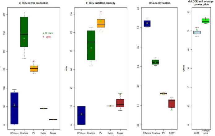
Testing weather sensitivity To test how the optimal mix of variable renewables varies for different weather-years, we ran the model for each year from 2000 to 2017 (henceforth “weather-years”). Our results show that the optimal power mix varies significantly from one year to another, both in terms of electricity production, installed capacity, storage volume and storage capacity (Figures 5 and 6 and Appendix 3). The largest variations between minimum and maximum installed capacity are associated with onshore and offshore wind power. In particular, offshore capacity ranges from zero to 20 GW,

20

which is the maximum value allowed1_{. High values for offshore wind are reached either for} weather-years with a high capacity factor for offshore wind (as in 2015) or for weather-years with a low capacity factor for onshore wind (as in 2016). In comparison, installed solar capacity is more stable (between 100.5GW and 122.2GW), due to a less volatile capacity factor (Figure 6c). Biogas always reaches the maximum allowed power generation and hydro the maximum allowed capacity. As far as storage capacity is concerned, pumped hydro storage (PHS) also always reaches its maximum value while batteries and methanation vary a lot across weather-years (Figures 6d1 and 6d2). In comparison, the system LCOE and average power price (the dual variable of the adequacy constraint, i.e. equation 3), as well as the sum of VRE curtailment and storage losses are much more stable (Figures 6e and 6f). Figure 5 VRE generation mix for each weather-year in single-year optimization and over the whole 18-year long period

1 _{Maximum values are not binding for solar PV and onshore wind.}

21

These results show that if the aim is to find an optimal energy mix, running a model on a randomly-chosen weather-year can be very misleading. The optimal mix of renewables is highly sensitive to the chosen weather-year. This conclusion is consistent with those of Collins et al. (2018) and Zeyringer et al. (2018). As the weather of future years cannot be predicted, the best approach would be to run the model over several weather-years, as in our 18-year simulation.

However, the drawback is a much longer optimization time, which prevents us from doing this for the 315 cost scenarios used in our sensitivity analysis. Hence we have chosen another approach: select a representative year that gives the results closest to the results when optimizing over 18 years.

Selecting a representative year

The selection of a representative year could be made using several criteria. We chose to select the year with a capacity factor closest to our 18-year optimal mix. We used the capacity factor because it is invariable with respect to technology costs, on which we perform the sensitivity analysis. To measure the distance to the 18-year optimal mix, we compute the sum of absolute difference1 _{of the three VREs.} Using this approach, 2006 is the closest year to the overall 18-year long period, with a sum of absolute error values of 1.5% (Table A.4). We launched the model with the optimal installed capacities found for 2006 over all other weather-years to test the adequacy of this installed capacity with respect to the other 17 weather-years, and we did not observe any operational inadequacy.

1 _{Sum of normalized absolute differences} /éâ/∗é /∗_é ê

\yZ where H\ is the CF of each technology 4 in each year and H∗\

22 Figure 6. Optimization results for each weather-year from 2000 to 2017 and for the whole 18-year period. (a) power production; (b) installed capacity; (c) average capacity factor of each VRE and the gas power plant for biogas produced by anaerobic digestion and methane produced by methanation and (d) system LCOE and average power price of electricity. The green dot shows the results of the optimization over the 18-year period and the red dot the results for weather-year 2006. The box plots show the first and third quartiles and the median for each scenario.

Figure 7 shows the energy mix of the chosen representative year (2006) and the whole 18-year modelling. There is a very close match between the percentage of each energy source for the overall 18-year-long optimization and the representative year. Onshore wind power is clearly dominant with solar power and offshore wind power as the second- and third- biggest sources of energy respectively.

23

4 Discussion & Conclusion

4.1 Comparison with existing studies

Some authors have argued that the storage facilities required for a fully renewable power system would massively increase the power system cost (e.g. Sinn, 2017, whose conclusions have been challenged by Zerrahn et al., 2018). In our reference cost scenario, storage (batteries, PHS and methanation) accounts for only 14.5% of the system cost, vs. 85.5% for electricity generation (Appendix 6). Moreover, we have seen that the system LCOE is much more robust to the cost of the storage technologies than to that of PV and wind. Hence the importance of the storage cost should not be overemphasized.

The system LCOE for power generation and storage ranges from €36 to €65/="ℎ#, depending on

technology costs, with an expected value between €50 and €52/="ℎ#, depending on whether the

power system is optimized before or after the arrival of information about technology costs. According to the latest quarterly report from the French energy regulator (CRE, 2018), 35% of a typical electricity bill represents electricity production, hence from a bill varying between €160 and €170/="ℎ#,

€56-€60/="ℎ# represents production. Hence the cost of a 100% renewable electricity system for France in

2050 would be lower than or similar to that of the current power system.

These results contrast with those of Krakowski et al. (2016) who find an annualized cost of more than €60 bn/yr. in their scenario 100RES2050 (cf. their Fig. 23) vs. €21 bn/yr. in ours. The explanation does not stem from their investment cost assumptions, which are similar to ours (cf. their Table 1). One explanation might be that they take a higher discount rate, but they do not disclose it so we cannot verify this hypothesis. Partial explanations are (i) a slightly higher power demand (cf. their Fig. 7: about 460 ("ℎ#/yr. vs. 422); (ii) a slightly lower capacity factor for onshore wind (28%) and offshore wind

(50%); (iii) the fact that they assume a perfect correlation between onshore and offshore wind production, which artificially limits the complementarity between these technologies. Moreover, they base their wind production profiles on observed power generation in 2012, which neglects the fact that advanced turbines generate electricity more constantly than those installed in the past (Hirth and Müller, 2016).

Villavicencio (2017), who does not specify the time horizon considered, finds even higher annualized cost: more than €180 bn/yr. for 100% renewables, i.e. more than 8 times our result. Several factors may explain this huge difference. First, he takes a real discount rate of 7%/yr. This is much higher than ours, which corresponds to the rate recommended for socio-economic analysis in France (4.5%). Second, his investment cost for PV is much higher than ours: €3.6/"#, while the current investment cost at utility scale is around $1/"# (Lazard, 2018). This explains why PV does not appear in his reference scenario (F1) with 100% renewables. Third, total demand is higher than ours (512 ("ℎ# vs. 422("ℎ#). To sum up, while our results point to a much lower system cost than the two above-mentioned studies modeling a 100% renewable system for France, there are good reasons to conclude that the system cost

24

for 2050 will be lower than that estimated by these studies. In the remainder of this subsection, we address several factors in turn which could push our estimates up or down.

4.2 Model limitations

Factors which could push costs up Cost of the transmission and distribution network Our system LCOE includes storage and connection of power generation to the grid, but not the cost of the transmission and distribution network. Currently this cost accounts for 27% of the typical electricity bill, i.e. about €45/="ℎ#. Calculating this cost for the various power systems considered in the present study would exceed the scope of the present article, but several recent studies indicate that the cost differential across scenarios featuring greater or lesser percentage of renewables would be limited. • According to the RTE systems and network perspectives study (2018), for a 71% renewable

electricity mix (the so-called Watt scenario for 2035) in France, the extra network costs would be in the order of €1 bn/yr., less than 5% of the total production cost. However, the relationship is not linear and it cannot be easily extrapolated for higher proportions of renewables. • According to two studies by ADEME (2015, 2018), the cost of renovating the French network, which is planned to take place before 2030, will be at least one order of magnitude more than the cost required to strengthen the grid for a fully renewable power network. • According to EirGrid1 _{(the Irish electricity network operator), for an electricity mix with nearly 90%} of renewables, the reinforcement required to integrate VREs will cost no more than €1/="ℎ#. Acceptability of wind power Our optimal scenario corresponding to the reference technology costs includes about 80 GW of onshore wind, 12 GW of offshore wind and 110 GW of PV. The availability of land for PV does not appear to be problematical since the amount of suitable land is much higher than required (Cerema, 2017). For offshore wind, WindEurope’s “high” scenario for 2030 forecasts 11 GW, roughly equivalent to our optimal scenario corresponding to the reference technology costs. Here again, reaching this capacity does not seem problematical. For onshore wind, WindEurope’s (2017) “high” scenario forecasts 41 GW in 2030, vs. 14 in 2018, i.e. an increase of 2.2 GW/yr. on average. Reaching 80 GW in 2050 means an increase of 2 GW/yr. on average, from 2018 onwards, a bit less than WindEurope’s “high” scenario, but almost twice the current rate of 1 _{http://www.eirgridgroup.com/newsroom/record-renewable-energy-o/index.xml}

25 increase. Sustaining such a high rate of increase requires a high degree of political determination, given the current opposition faced by many wind projects in France. Discount rate Some studies use higher discount rates than ours, e.g. 7% in Villavicencio (2017), as mentioned above. This would increase the annualized LCOE, and especially the cost of capital-intensive technologies. While higher rates may well be used by private companies, 4.5% is already much higher than both the rate-free real interest rate available on financial markets, and expected GDP growth over the next few decades. Using a higher rate in a socioeconomic analysis means than future generations would be penalized when compared to current ones, which can hardly be defended on ethical grounds.

Perfect weather forecasts

Our optimization has been conducted on the assumption that the weather is known for the whole period. With imperfect weather forecasts, the cost would be higher, but such an optimization for a country-scale system would be computationally challenging. Gowrisankaran et al. (2016) have performed such an optimization just for solar energy, on a limited geographical scale, and have found that “intermittency overall is quantitatively much more important than unforecastable intermittency.” However, whether this conclusion would hold for a complex, multi-energy system is an open question.

Factors which could bring costs down

Demand-side management

Our model does not feature price-elastic electricity demand or flexibility in the power consumption profile, because this would have required debatable assumptions. Moreover, the demand profile, taken from ADEME (2015), is already flatter than the current one. Including these features would reduce the need for storage and the related energy losses. Interconnection with neighboring countries Many studies have shown that interconnections with neighboring countries can significantly reduce the cost of a fully renewable system. For instance, Annan-Phan and Roques (2018) have shown that power price volatility can be reduced by cross-border exchanges with neighboring countries. Indeed, this leads to benefits from the differences both in climatic and weather conditions between the countries concerned.

26

Spatial optimization of renewable energy capacities

As mentioned above, we do not optimize the quantity of renewables at every location but only the aggregate capacity, which is thus scaled up compared to the value observed in 2017. A lower system cost would be obtained by optimizing their location, which would presumably lead to greater capacity in windier or sunnier locations, although this effect would be mitigated by the need to obtain a flatter aggregate generation profile. Yet this would make the model computationally intractable and might lead to unrealistic concentrations of onshore wind in some locations. Neither vehicle-to-grid nor second-hand batteries We have not considered vehicle-to-grid i.e. the possibility that electric vehicle batteries could be used to provide flexibility in the electricity system. Yet the storage capacity of electric vehicles may be huge by 2050: The French TSO RTE (2018) estimates it at 900 ("ℎ#, about ten times the battery capacities in our reference cost scenario. Mobilizing even a small part of this capacity for power storage would bring down the system LCOE, but we have preferred not to include this option because the impact on battery lifetime is still being debated. Another possibility is to recycle used car batteries as stationary batteries, but again, we believe that modeling this option would require precise assumptions on battery degradation.

4.3 Conclusion

In this article, we have studied the sensitivity of optimal fully renewable power systems to technology cost. To that end, we have developed EOLES, a model optimizing investment and dispatch in the power sector, and applied it to the study of fully renewable power systems in France. We built 315 cost scenarios by combining assumptions about the long-term cost of the key power generation and storage technologies.

Our results indicate that even though the technologies involved in a fully renewable power system are very different, they are by and large substitutable. For instance, if batteries are 50% more expensive than expected, the optimal energy mix includes fewer batteries and less PV, but this is compensated for by additional wind power, with a very limited impact on the system LCOE. On the contrary, if wind power is 25% more expensive than expected, the optimal mix obviously includes less of this technology, but this is compensated for by more PV and storage.

Overall, the impact of storage cost should not be overestimated: even in a 100% renewable power system, storage (batteries, PHS and methanation) accounts for only 14.5% of the system cost, vs. 85.5% for electricity generation. Were our model to include demand-side management, interconnections with

27

neighboring countries, vehicle-to-grid or second-hand batteries, the share of storage in overall cost would be even lower.

Across all cost scenarios, the system LCOE, including generation and storage, ranges from €36.5 to €65.5/="ℎ#, depending on the cost scenario, with an average value of €50/="ℎ#. This is cheaper

than today’s value. And setting a capacity target in advance for every technology would only increase the system LCOE by €2/MWh averaged over the 315 cost scenarios compared to the optimum mix, even if costs vary by +/-25% for wind and +/-50% for solar and storage. In terms of policy implications, this result calls for providing visibility to investors, even if it entails reducing flexibility the policy design. Finally, our analysis shows that the optimal power mix is highly sensitive to the chosen weather-year and to the cost assumptions. In the literature, many analyses of the power mix are still based on a unique weather-year, chosen for data availability rather than representativeness. Our result thus calls for caution over such conclusions on the optimal power mix, when they are based on a limited number of weather-years or cost scenarios.

This work could be extended in many directions, for example including the other power generation technologies that entail low direct CO2 emissions: CO2 capture and storage and nuclear power. Their cost and the possibility of storing massive quantities of CO2 being very uncertain in the French context,

28

References

ADEME (2013). L’exercice de prospective de l’ADEME “Vision 2030-2050” - document technique. ADEME (2015). Vers un mix électrique 100 % renouvelable. https://www.ademe.fr/sites/default/files/assets/documents/mix-electrique-rapport-2015.pdf. ADEME (2018). Trajectoires d'évolution du mix électrique à horizon 2020-2060. ISBN: 979-10-297-1173-2 Annan-Phan, S., & Roques, F. A. (2018). « Market Integration and Wind Generation: An Empirical Analysis of the Impact of Wind Generation on Cross-Border Power Prices.” The Energy Journal 39(3), 1-25. Arditi, M., Durdilly, R., Lavergne, R., Trigano, É., Colombier, M., Criqui, P. (2013). Rapport du groupe de travail 2: Quelle trajectoire pour atteindre le mix énergétique en 2025 ? Quels types de scénarios possibles à horizons 2030 et 2050, dans le respect des engagements climatiques de la France ? Tech. rep., Rapport du groupe de travail du conseil national sur la Transition Energétique. Brown, T. W., Bischof-Niemz, T., Blok, K., Breyer, C., Lund, H., & Mathiesen, B. V. (2018). Response to ‘Burden of proof: A comprehensive review of the feasibility of 100% renewable-electricity systems’. Renewable and sustainable energy reviews, 92, 834-847. Cerema, 2017. Photovoltaïque au sol. https://www.collins.fr/fr/actualites/photovoltaique-au-sol Collins, S., Deane, P., Gallachóir, B. Ó., Pfenninger, S., & Staffell, I. (2018). “Impacts of inter-annual wind and solar variations on the European power system.” Joule 2(10), 2076-2090. CRE (2018). Observatoire des marchés de détail de l’électricité et du gaz naturel du 3e trimestre 2018. https://www.cre.fr/content/download/20125/256999. ENEA Consulting (2016). The potential of Power-to-Gas. https://www.enea-consulting.com/sdm_downloads/the-potential-of-power-to-gas/ ENTSO-E (2013). Network Code on Load-Frequency Control and Reserves 6, 1–68. Ericsson, K. (2017). “Biogenic carbon dioxide as feedstock for production of chemicals and fuels: A techno-economic assessment with a European perspective.” Environmental and Energy System Studies, Lund University: Miljö- och energisystem, LTH, Lunds universitet. FCH JU (2015). Commercialisation of energy storage in Europe: Final report.

29 Gowrisankaran, G., Reynolds, S. S., & Samano, M. (2016). Intermittency and the value of renewable energy. Journal of Political Economy, 124(4), 1187-1234. Henze, V., 2019. Battery Power’s Latest Plunge in Costs Threatens Coal, Gas. https://about.bnef.com/blog/battery-powers-latest-plunge-costs-threatens-coal-gas/ Hirth, L. (2015): “The Optimal Share of Variable Renewables”. The Energy Journal 36(1), 127- 162. doi:10.5547/01956574.36.1.6. Hirth, L., & Müller, S. (2016). System-friendly wind power: How advanced wind turbine design can increase the economic value of electricity generated through wind power. Energy Economics, 56, 51-63. Huld T, Gottschalg R, Beyer HG, Topič M. (2010). “Mapping the performance of PV modules, effects of module type and data averaging.” Solar Energy 2010;84(2):324–38. Joskow, P. L. (2011). Comparing the costs of intermittent and dispatchable electricity generating technologies. American Economic Review, 101(3), 238-41. JRC (2014) Energy Technology Reference Indicator Projections for 2010–2050. EC Joint Research Centre Institute for Energy and Transport, Petten. JRC (2017) Cost development of low carbon energy technologies - Scenario-based cost trajectories to 2050, EUR 29034 EN, Publications Office of the European Union, Luxembourg, 2018, ISBN 978-92-79-77479-9, doi:10.2760/490059, JRC109894. Jülch, V., Telsnig, T., Schulz, M., Hartmann, N., Thomsen, J., Eltrop, L., & Schlegl, T. (2015). A holistic comparative analysis of different storage systems using levelized cost of storage and life cycle indicators. Energy Procedia, 73, 18-28. Krakowski, V., Assoumou, E., Mazauric, V., & Maïzi, N. (2016). “Feasible path toward 40–100% renewable energy shares for power supply in France by 2050: A prospective analysis.” Applied energy 184, 1529-1550. Lauret P, Boland J, Ridley B. (2013). “Bayesian statistical analysis applied to solar radiation modelling.” Renewable Energy 2013;49:124–7. Moraes, L., Bussar, C., Stoecker, P., Jacqué, K., Chang, M., & Sauer, D. U. (2018). “Comparison of long- term wind and photovoltaic power capacity factor datasets with open-license.” Applied Energy 225, 209-220. Perrier, Q. (2018). “The second French nuclear bet.” Energy Economics, 74, 858-877.

30 Pfenninger, S., Staffell, I. (2016). “Long-term patterns of European PV output using 30 years of validated hourly reanalysis and satellite data.” Energy 114, pp. 1251-1265. doi: 10.1016/j.energy.2016.08.060 Pierrot M. (2018). The wind power. http://www.thewindpower.net Quinet, E. (2014). L'évaluation socioéconomique des investissements publics (No. Halshs 01059484). HAL. Rienecker M.M., Suarez M.J., Gelaro R., Todling R., Bacmeister J., Liu E., et al. (2011). “MERRA: NASA’s modern-era retrospective analysis for research and applications.” J Climate 2011;24(14):3624–48 Rogelj J, Shindell D, Jiang K, Fifita S, Forster P, Ginzburg V, Handa C, Kheshgi H, et al.(2018). Chapter 2: Mitigation pathways compatible with 1.5 C in the context of sustainable development. In: Global Warming of 1.5 C - an IPCC special report on the impacts of global warming of 1.5 C above pre-industrial levels and related global greenhouse gas emission pathways, in the context of strengthening the global response to the threat of climate change. Intergovernmental Panel on Climate Change. RTE, commission perspective système et réseau (2018). Point d’étape sur les travaux du bilan prévisionnel et du schéma décennal de développement réseau. https://www.concerte.fr/system/files/concertation/2018%2009%2028%20CPSR_complet2.pdf RTE (2018), Panorama de l’électricité renouvelable au 30 Juin 2018. Schlachtberger, D.P., Brown, T., Schäfer, M., Schramm, S., Greiner, M. (2018). “Cost optimal scenarios of a future highly renewable European electricity system: Exploring the influence of weather data, cost parameters and policy constraints.” arXiv preprint arXiv:1803.09711. Schmidt, O., Melchior, S., Hawkes, A., Staffell, I. (2019). “Projecting the Future Levelized Cost of Electricity Storage Technologies.” Joule ISSN 2542-4351 https://doi.org/10.1016/j.joule.2018.12.008 Sinn, H. W. (2017). Buffering volatility: A study on the limits of Germany's energy revolution. European Economic Review, 99, 130-150. Staffell, I., Pfenninger, S. (2016). “Using Bias-Corrected Reanalysis to Simulate Current and Future Wind Power Output.” Energy 114, pp. 1224-1239. doi: 10.1016/j.energy.2016.08.068 Van Stiphout, A., De Vos, K., & Deconinck, G. (2017). “The impact of operating reserves on investment planning of renewable power systems.” IEEE Transactions on Power Systems, 32(1), 378-388. Villavicencio, M. (2017). “A capacity expansion model dealing with balancing requirements, short-term operations and long-run dynamics.” CEEM Working Papers (Vol. 25).

31 WindEurope (2017). Wind energy in Europe, Scenarios for 2030. 22 September. https://windeurope.org/about-wind/reports/wind-energy-in-europe-scenarios-for-2030/ Wiser, R., Jenni, K., Seel, J., Baker, E., Hand, M., Lantz, E., & Smith, A. (2016). “Expert elicitation survey on future wind energy costs.” Nature Energy 1(10), 16135. ZEP (2011). The Costs of CO2 Transport. Post-demonstration CCS in the EU. Zero Emissions Platform. http://www.zeroemissionsplatform.eu/downloads/813.html Zerrahn, A., Schill, W. P., & Kemfert, C. (2018). On the economics of electrical storage for variable renewable energy sources. European Economic Review, 108, 259-279. Zeyringer, M., Price, J., Fais, B., Li, P. H., & Sharp, E. (2018). “Designing low-carbon power systems for Great Britain in 2050 that are robust to the spatiotemporal and inter-annual variability of weather”. Nature Energy 3 (5), 395.

32

Appendix 1. Additional information on the JRC 2017 study

In this JRC report, historic installed capacity of each technology for 2015, learning rate related to each technology and the capital investment cost of each technology in 2015 has been taken as input values, and using three different future installed capacity scenarios, three different future cost trajectories are proposed. Equation (A1) shows the main methodology used in the cost projection using the learning rate method:

%ëI5₊ = %ëI5_z∙ Ç_

Çì

î

(A1)

This log-linear relation relates the future cost (%ëI5+) of a technology to the existing cost (%ëI5z),

existing installed capacity (%z) and the future projected installed capacity (%+) of it using the experience

parameter i. The learning rate LR is related to the experience parameter as it is described in equation (A2); ;U = 1 − 2î _(A2) The JRC report uses three different scenarios to project the future installed capacity of each technology, and finally to find the Ç_ Çì ratio for the equation (16). These three scenarios are described in Table A-1; Table A-1 the chosen scenarios by JRC for the 2050 cost projections of low carbon power production technologies Scenario

Baseline This scenario is used to cover the lower end of RES-E deployment. It is based on the "6DS" scenario of the Energy Technology Perspectives published by the International Energy Agency in 2016. It represents a "business as usual" world in which no additional efforts are taken on stabilizing the atmospheric concentration of greenhouse gases. By 2050, primary energy consumption reaches about 940 EJ, renewable energy supplies about 30 % of global electricity demand and emissions climb to 55 GtCO2.

Diversified The "Diversified" portfolio scenario is taken from the "B2DS" scenario of the

International Energy Agency's 2017 Energy Technology Perspectives and is used as representative for the mid-range deployment of RES-E found in literature. To achieve rapid decarbonization in line with international policy goals, all known supply, efficiency and mitigation options are available and pushed to their practical limits. Fossil fuels and nuclear energy participate in the technology mix, and CCS is a key option to realize emission reduction goals. Primary energy consumption is comparable to 2015 levels (about 580 EJ), the share of renewable electricity in the global supply mix is 74 % while emissions decline to about 4.7 GtCO2 by 2050.

ProRES The "ProRES" scenario results are the most ambitious in terms of capacity additions of RES-E technologies. In this scenario the world moves towards decarbonization by significantly reducing fossil fuel use, however, in parallel with rapid phase out of nuclear power. CCS does not become commercial and is not an available mitigation option. Deep

33 emission reduction is achieved with high deployment of RES, electrification of transport and heat, and high efficiency gains. It is based on the 2015 "Energy Revolution" scenario of Greenpeace. Primary energy consumption is about 430 EJ, renewables supply 93 % of electricity demand and global CO2 emissions are about 4.5 GtCO2 in 2050.

The used economical parameters for the power production technologies are taken from the 2050 projections of this study for the diversified scenario as an average and more realistic scenario.

34

Appendix 2. Wind and solar production profiles

The wind power hourly capacity factor profiles existing in the renewables.ninja website are prepared in four stages: a) Raw data selection; using NASA’s MERRA-2 data reanalysis with a spatial resolution of 60km×70km provided by Rienecker et al. (2011), b) Downscaling the wind speeds to the wind farms; by interpolating the specific geographic coordinates of each wind farm using LOESS regression, c) Calculation of hub height wind speed; by extrapolating the wind speed in available altitudes (2, 10 and 50 meters) to the hub height of the wind turbines using logarithm profile law, d) Power conversion; using the primary data from Pierrot (2018), the power curves are built (with respect to the chosen wind turbine), and smoothed to represent a farm of several geographically dispersed turbines using Gaussian filter. The solar power hourly capacity factor profiles in the renewables.ninja website are prepared in three stages: a) Raw data calculation and treatment; using NASA’s MERRA data with the spatial resolution of 50km×50km. The diffuse irradiance fraction estimated with Bayesian statistical analysis introduced by Lauret et al. (2013) and the global irradiation calculated in inclined plane. The temperature is given at 2m altitude by MERRA data set. b) Downscaling of solar radiation to farm level; values are linearly interpolated from grid cells to the given coordinates. c) Power conversion model; Power output of a panel is calculated using the relative PV performance model by Huld et al. (2010) which gives temperature dependent panel efficiency curves.

35

Appendix 3. Weather year sensitivity

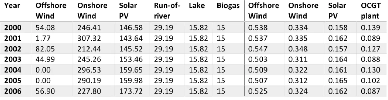
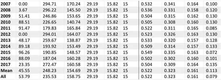
The results for each weather year can be seen in Tables A.1 and A.2, A.3. Table A.1 installed capacity of each power production technology in GWe and energy storage capacity of each storage technology during each optimization period Year Offsho re Wind Onshor

e Wind Solar PV Run-of-river Lake & reservoi r Bioga s Battery (GWh) PHS (GWh ) Methanatio n (TWh) 2000 11.46 84.14 105.74 7.50 13.00 18.24 60.17 180 5.52 2001 0.38 104.62 101.16 7.50 13.00 28.61 41.91 180 8.45 2002 17.12 69.66 105.55 7.50 13.00 19.16 74.70 180 4.60 2003 10.21 90.15 106.83 7.50 13.00 25.70 62.78 180 5.52 2004 0.00 105.29 113.38 7.50 13.00 21.88 70.32 180 15.30 2005 0.00 105.89 110.38 7.50 13.00 25.22 60.27 180 9.37 2006 12.36 80.08 122.17 7.50 13.00 32.89 74.62 180 12.90 2007 0.00 98.40 118.33 7.50 13.00 27.61 65.73 180 12.05 2008 0.78 101.95 105.20 7.50 13.00 21.76 52.03 180 12.05 2009 11.61 89.32 107.79 7.50 13.00 18.83 51.47 180 6.92 2010 20.00 83.64 100.50 7.50 13.00 22.88 40.53 180 15.81 2011 20.00 65.81 114.17 7.50 13.00 28.32 101.33 180 8.54 2012 0.00 103.38 114.49 7.50 13.00 20.36 62.43 180 11.32 2013 10.32 92.30 100.82 7.50 13.00 21.54 37.06 180 10.59 2014 20.00 70.23 111.40 7.50 13.00 18.57 80.03 180 7.69 2015 20.00 64.77 103.78 7.50 13.00 34.09 63.19 180 8.22 2016 20.00 69.77 114.07 7.50 13.00 23.96 81.68 180 8.66 2017 5.29 100.72 111.62 7.50 13.00 19.30 50.05 180 11.77 Mean 9.97 87.78 109.30 7.50 13.00 23.83 62.79 180 7.74 All 11.77 83.30 112.21 7.50 13.00 33.25 66.71 180 16 Table A.2 Yearly power production of each production technology (in TWh) and capacity factor of VRE resources Year Offshore

Wind Onshore Wind Solar PV Run-of-river Lake Biogas Offshore Wind Onshore Wind Solar PV OCGT plant

2000 54.08 246.41 146.58 29.19 15.82 15 0.538 0.334 0.158 0.139 2001 1.77 307.32 143.64 29.19 15.82 15 0.537 0.335 0.162 0.089 2002 82.05 212.44 145.52 29.19 15.82 15 0.547 0.348 0.157 0.127 2003 44.99 245.26 153.46 29.19 15.82 15 0.503 0.311 0.164 0.088 2004 0.00 296.53 159.65 29.19 15.82 15 0.509 0.322 0.161 0.130 2005 0.00 290.19 159.98 29.19 15.82 15 0.507 0.312 0.165 0.102 2006 56.90 227.80 173.72 29.19 15.82 15 0.525 0.324 0.162 0.087