Publisher’s version / Version de l'éditeur:
Vous avez des questions? Nous pouvons vous aider. Pour communiquer directement avec un auteur, consultez la
première page de la revue dans laquelle son article a été publié afin de trouver ses coordonnées. Si vous n’arrivez
Questions? Contact the NRC Publications Archive team at
PublicationsArchive-ArchivesPublications@nrc-cnrc.gc.ca. If you wish to email the authors directly, please see the first page of the publication for their contact information.
https://publications-cnrc.canada.ca/fra/droits
L’accès à ce site Web et l’utilisation de son contenu sont assujettis aux conditions présentées dans le site LISEZ CES CONDITIONS ATTENTIVEMENT AVANT D’UTILISER CE SITE WEB.
Indoor Air Quality Problems and Engineering Solutions 2003 [Proceedings], pp. 1-17, 2003-07-01
READ THESE TERMS AND CONDITIONS CAREFULLY BEFORE USING THIS WEBSITE. https://nrc-publications.canada.ca/eng/copyright
NRC Publications Archive Record / Notice des Archives des publications du CNRC :
https://nrc-publications.canada.ca/eng/view/object/?id=1bf7028c-b9c9-4058-a5b8-6199690dde32 https://publications-cnrc.canada.ca/fra/voir/objet/?id=1bf7028c-b9c9-4058-a5b8-6199690dde32
Archives des publications du CNRC
This publication could be one of several versions: author’s original, accepted manuscript or the publisher’s version. / La version de cette publication peut être l’une des suivantes : la version prépublication de l’auteur, la version acceptée du manuscrit ou la version de l’éditeur.
Access and use of this website and the material on it are subject to the Terms and Conditions set forth at
VOC emission from building materials - the impact of specimen variability - a case study
VOC emissions from building materials – the impact of specimen variability – a case study
Magee, R.J.; Won, D.; Shaw, C.Y.; Lusztyk, E.; Yang, W.
NRCC-47061
A version of this document is published in / Une version de ce document se trouve dans : Indoor Air Quality Problems and Engineering Solutions,
Research Triangle Park, N.C., July 21-23, 2003, pp. 1-17
VOC Emissions from building materials - the impact of
specimen variability - a case study.
RJ Magee, D Won, CY Shaw, E Lusztyk, W Yang
Indoor Environment Research Program, Institute for Research in Construction, National Research Council of Canada, 1200 Montreal Road, Ottawa, Ont. Canada K1A OR6 Phone: (613) 993-9631, Fax (613) 954-3733, Email: bob.magee@nrc.ca
ABSTRACT
Significant progress has been made in the development of standardized methods for the testing and analysis of volatile organic compound (VOC) emission characteristics of different building materials. These standardized techniques facilitate product-product comparisons with regard to VOC emissions, and also provide a basis with which to examine the impact of environmental conditions on VOC emissions. Variability of the test specimen itself is one factor that must be considered when evaluating such tests. In an attempt to gauge this effect, a series of samples of oriented strand board (OSB) were collected and subjected to chamber tests for VOC emissions under standardized conditions (23oC, 50% RH, 1 air change per hour, 0.4 m2/m3 loading). Specimens were collected directly from the mill sites of three different manufacturers. Repeat samples were also collected from the same retail outlet on three separate occasions (same manufacturer, 3 different production dates), from separate panels produced on the same production date, and from multiple locations within the same panel. Variability in the VOC emissions from these samples was found to exceed the analytical uncertainty by an order of magnitude in certain cases.
INTRODUCTION
Testing of chemical emissions from building materials is increasingly conducted to assist with the design, construction and renovation of buildings so as to provide optimal indoor
environments.1 The growing number of labeling schemes which attempt to rank products based on their VOC emissions,2,3,4 and of databases seeking to catalog emission test results,5,6,7,8 underscores the need for reliable, standardized testing protocols.9 Several detailed guidance documents are currently available to describe such tests,10,11 but by definition, their
recommendations are non-mandatory and consequently, many reported test results are neither repeatable nor comparable. Strict procedures for, and documentation of, specimen collection, handling, conditioning, and chamber characterization/operation are vital, as are precise control of VOC sampling and analysis techniques in maximizing uniformity and comparability of reported emissions data. Efforts to meet these challenges continue.12,13,14,15
Even if such tight control of testing procedures is achieved, some variability in the observed chemical emissions for a given building material is still to be expected.16 Material
in-homogeneity is at least partially blamed for some of the inconsistent results obtained in several recent round robin lab evaluations.17,18 Variability in the raw materials used in manufacture, and in the manufacturing processes themselves leads to non-uniformity in the emission
characteristics of many building materials. OSB, widely used in the construction industry, is one example of a product which is relatively in-homogeneous. OSB is a complex mixture of a
variety of wood species (typically aspen-poplar or yellow birch), phenol-formaldehyde resins (or equivalents) and waxes. A variety of mechanical techniques and processing conditions are employed in the manufacture of the panels. In a study on the impact of furnish drying
temperature, moisture content, panel pressing time, pressing temperature and resin content on VOC emissions from OSB panels, drying temperature in particular was found to have a significant impact on VOC emissions from the finished material.19
A series of tests of OSB were conducted, under carefully controlled conditions, to examine the degree of variability that can occur in the emissions of VOCs from a single building product. This comparison is material-dependent, but has general impact on the manner in which emission results are presented and on the way in which emissions databases and material labeling schemes rate their inventories.
EXPERIMENTAL METHODS
Specimen Selection and Handling
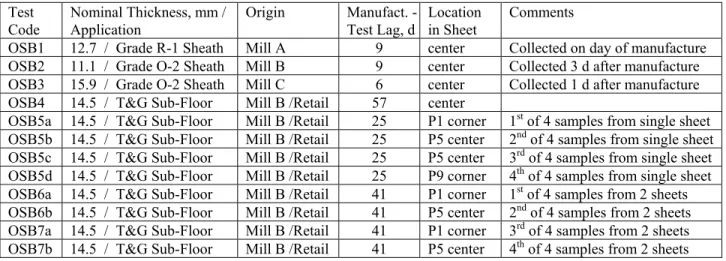
OSB specimens were obtained from a variety of sources (summarized in Table 1). Specimens 1, 2 and 3 were collected directly from mill production sites under strict quality control
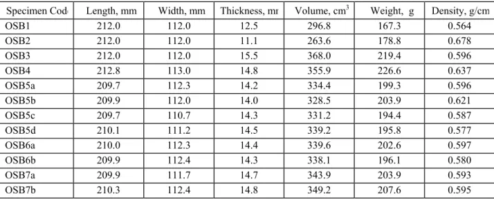
procedures.13 Specimens 4 through 7 were all purchased from a large retail outlet close to the testing lab. For each of these specimens, an OSB panel near the center of an undisturbed stack of panels was collected along with the two immediately adjacent panels (which were clamped together with the test panel to form a protective sandwich). On receipt at the lab, 112 by 212 mm test specimens were immediately cut from the panel with a clean saw (using the sandwich panels as work surfaces) and stored in clean sample bags; flushed with zero-grade air, and stored at 23oC for a minimum 48 hours prior to chamber testing. The cut dimensions of the specimens
are provided in Table 2. Immediately prior to chamber testing, the specimens were placed in an electropolished stainless steel holder.13 The holder served to restrict the emitting surface of the specimen to an area of 100 x 200 mm, and also prevented emissions from the side and bottom faces of the specimen. For samples 4 through 7, the “this side down” face of the panel was exposed to the chamber, since in typical residential construction; this would be the primary exposed surface (looking up at the exposed sub-floor from the basement).
Table 1. Specimen description. Test Code Nominal Thickness, mm / Application Origin Manufact. -Test Lag, d Location in Sheet Comments
OSB1 12.7 / Grade R-1 Sheath Mill A 9 center Collected on day of manufacture OSB2 11.1 / Grade O-2 Sheath Mill B 9 center Collected 3 d after manufacture OSB3 15.9 / Grade O-2 Sheath Mill C 6 center Collected 1 d after manufacture OSB4 14.5 / T&G Sub-Floor Mill B /Retail 57 center
OSB5a 14.5 / T&G Sub-Floor Mill B /Retail 25 P1 corner 1st of 4 samples from single sheet
OSB5b 14.5 / T&G Sub-Floor Mill B /Retail 25 P5 center 2nd of 4 samples from single sheet
OSB5c 14.5 / T&G Sub-Floor Mill B /Retail 25 P5 center 3rd of 4 samples from single sheet
OSB5d 14.5 / T&G Sub-Floor Mill B /Retail 25 P9 corner 4th of 4 samples from single sheet
OSB6a 14.5 / T&G Sub-Floor Mill B /Retail 41 P1 corner 1st of 4 samples from 2 sheets
OSB6b 14.5 / T&G Sub-Floor Mill B /Retail 41 P5 center 2nd of 4 samples from 2 sheets
OSB7a 14.5 / T&G Sub-Floor Mill B /Retail 41 P1 corner 3rd of 4 samples from 2 sheets
Chamber Testing
Four identical electropolished stainless steel chambers with internal volumes of 0.050 m3 were
used in this study according to the guidelines of ASTM D5116.10 Chamber conditions for all
tests were 23oC, 50% relative humidity and a nominal air change rate of 1.0 h-1 (~1.04 h-1 after correction for volume occupied by the specimen and specimen holder). Mass flow controllers regulated the chamber supply air from an Aadco pure air generator which was humidified to 50% RH with HPLC grade water. This system produced clean air with TVOC values below 20 µg/m3 and individual VOC levels below 0.5 µg/m3. Chamber differential pressure was continuously monitored to maintain a slight positive pressurization (approximately 10 Pa) throughout each test. Tests 5a,b,c and d were conducted simultaneously in these four chambers, as were Tests 6a, 6b, 7a, and 7b, to prevent any impact of sample age or storage conditions from affecting the specimen variability results.
Table 2. Dimensions of test specimens.
Specimen Code Length, mm Width, mm Thickness, mm Volume, cm3 Weight, g Density, g/cm3
OSB1 212.0 112.0 12.5 296.8 167.3 0.564 OSB2 212.0 112.0 11.1 263.6 178.8 0.678 OSB3 212.0 112.0 15.5 368.0 219.4 0.596 OSB4 212.8 113.0 14.8 355.9 226.6 0.637 OSB5a 209.7 112.3 14.2 334.4 199.3 0.596 OSB5b 209.9 112.0 14.0 328.5 203.9 0.621 OSB5c 209.7 110.7 14.3 331.2 194.4 0.587 OSB5d 210.1 111.2 14.5 339.2 195.8 0.577 OSB6a 210.0 112.3 14.4 339.6 202.6 0.597 OSB6b 209.9 112.4 14.3 338.1 196.1 0.580 OSB7a 209.9 111.7 14.7 343.9 203.9 0.593 OSB7b 210.3 112.4 14.8 349.2 207.6 0.595
VOC Sampling and Analysis
A detailed description of the analytical methodology used in this study has been previously reported.20 A summary of the methods is given below.
Chemical Analysis
VOCs from the chamber tests of the OSB specimens were monitored by two separate methodologies: GC/MS and HPLC.
GC/MS Analysis
Sample collection and analysis: Air samples were collected from the dynamic chamber on multilayer Carbotrap 300 tubes, and subsequently desorbed on a Perkin-Elmer ATD400 thermodesorber and analyzed by a Gas Chromatography/Mass Spectroscopy. DB-5 60 m capillary columns (0.25µm film thickness, 0.32 mm ID) were used for separation of VOCs. For tests 1, 2, 3, an HP 5989 MS Engine was used; desorption temperature was 320oC; GC oven
temperature program was from 100oC to 250oC. Tests 4, 5, 6, and 7 were analyzed by an Agilent Technologies MSD 5973; desorption temperature was 350oC; and GC oven temperature
program was from –20 to 280oC. For all tests, a three-point calibration using a standard mixture, which included toluene, was performed each time samples were analyzed.
GC/MS qualitative analysis: Identification of emitted compounds from all tests was done for samples taken after 24 h from the beginning of each test. Individual VOCs were identified by comparison of the peak’s MS spectrum with the NIST98 library coupled with ChemStation software. Peak retention times, published data and previous analytical experience helped to validate the identification. In some cases, full identification was not possible.
GC/MS quantitative analysis: Two levels of quantification were performed.
Relative concentrations of identified VOCs were determined as the percentage of individual peak counts vs. the total peaks counts. These results should be viewed as semi-quantitative only. In many cases, co-elution of peaks resulted in significant integration error.
For ten selected VOCs and TVOC, a more precise quantification was performed. Heptanal, hexanal and α-pinene concentrations were calculated using their extracted ion response factors. The toluene response factor was used for pentanal; formic acid, pentyl ester; 2-heptanone; furan, 2-pentyl; 2-octenal; acetic acid; and hexanoic acid. TVOC was also quantified using the toluene response factor, but with a separately conducted integration of all peaks together. HPLC Analysis
For determination of aldehydes and carbonyl compounds, samples from the chamber exhaust air were collected on DNPH-treated SPE cartridges (Waters SepPak XPoSure Aldehyde), extracted with acetonitrile and analyzed by HPLC (Varian 9012 Solvent Delivery System / 9050 Variable Wavelength UV-VIS Detector (at 360nm) / Prostar 410 Autosampler. Two Supelcosil LC-18 columns (25cm x 4.6mm, 5 µm) in series at 30oC were used to run a gradient of acetonitrile in water from 60% to 100%. Identification and quantification of target compounds was performed via injection of pure individual standards and calibration of the system using TO-11/IP-6A Aldehyde/Ketone reference standards (Supelco). HPLC analysis was performed for test 4-7.
Data Analysis/Modeling:
Previous work demonstrated that a power law model best describes the emission of VOCs from dry building materials.21,22,23,24 Regression analysis was therefore performed to determine a
power law fit of the concentration vs. time data (elapsed time > 24 h) for each compound/test according to the equation:
Ct = ac tb (1)
where:
Ct = chamber concentration of VOC (or TVOC) at time t, mg/m3
ac = empirical constant
Standard error values (R2) for each curve were calculated as indicators of agreement with the power law behavior, and also of analytical variability.
Several methods are possible for calculating VOC emission factors 10, but for dry materials, where concentration change over time is relatively small, the emission factor at time t can be directly calculated from concentration data 24 using the following equation:
Et = Ct N/L (2)
where:
Et = emission factor at time t, mg/m2h
N = chamber air change rate per hour, h-1
L = product loading ratio (exposed surface area / chamber volume), m2/m3 Plotting the values of Et vs. t and using non-linear regression to fit a power law function to the data yields the following general expression for the power law decay model:
Et = a t-k (3)
where:
a = empirical constant
k = decay constant, dimensionless
Comparison of equation 1, 2, and 3 shows that a = ac (N/L); and k = -b. Thus, for these
conditions, the power law decay coefficients can also be calculated directly from the concentration vs. time power law fit.
Experimental Uncertainty Analysis
In order to be able to evaluate emission variability on a specimen by specimen basis, it was first necessary to estimate the uncertainty in the measured VOC concentrations due either to sampling techniques and quantification (GC/MS or HPLC), or due to experimental uncertainties related to control of the chamber environmental conditions. These uncertainty determinations are
discussed below. GC/MS Measurements
The emission factor from a dynamic material emission chamber test with a steady state can be calculated based on Eq. (4):
ct t c s s RFR A V A Q V M A Q C A Q E= = = 1 (4)
where E is emission factor (mg/m2/h); Q is the chamber flow rate (m3/h); A is the surface area of a specimen (m2); C is the chamber air concentration (µg/m3); M is the mass in the air sample collected in a sorbent tube (µg); Vs is the sampling volume (m3). Ac is the area under the curve of a selected ion of a compound of interest (area); RFt91 is the response factor of the ion with a
ratio of the response factor of a selected ion of a chemical of interest against that of the ion with the mass-to-charge ratio of 91 of toluene.
The variance of E can be expressed in terms of the variances of the quantities calculated from experimental data associated with each term on the right side of Eq. (4):
2 2 2 2 2 2 2 2 2 2 2 2 2 ct t c s R ct RF t A c V s A Q E R E RF E A E V E A E Q E σ σ σ σ σ σ σ ∂ ∂ + ∂ ∂ + ∂ ∂ + ∂ ∂ + ∂ ∂ + ∂ ∂ = (5)
where σE2 is the variance of E (mg/m2h), σA2 is the variance of A (m2); σVs2 is the variance of Vs
(m3); σAc2 is the variance of Ac (m2); σRFt2 is the variance of RFt; σRct2 is the variance of Rct
(1/mg);
In general, the uncertainty of A and Vs is considered insignificant, i.e., σA ≈0 and σVS ≈0.
Therefore, the uncertainty (U) associated with E can be simplified as:
2 2 2 2 2 2 2 2 ct t c R ct RF t A c Q E R E RF E A E Q E U σ σ σ σ σ + + + = = (6)
The relative uncertainty (Ur) with the unit of % can be expressed as:
2 2 2 2 100 100 + + + = = CT R T RF c A Q E r R RF A Q E U σ σ σ c σ T σ CT (7)
According to the measurements, Q Q σ ≈ 0.1%, c A A C σ ≈ 1%, and T RF RF t σ ≈ 10%.
The term σQ was calculated from the flow rate data recorded during a chamber test. The term
σAc was obtained from 20 trials of manual integration of a chromatograph peak. The term σRFt
was determined from three sets of three-points calibration curves run for a set of chamber test. The term, σRct , was obtained from standard calibrations run over a period of one year.
Uncertainty Analysis for HPLC Measurements
The emission factor from a dynamic material emission chamber test with a steady state can be calculated based on Eq. (8) for the HPLC analysis.
c c s s RF A V A Q V M A Q C A Q E= = = 1 (8) where RFc is the response factor of the chemical of interest. The response factor for each
compound was obtained from an external calibration with five concentration levels.
With the same procedure for the uncertainty analysis for GC/MS measurements, the relative uncertainty for HPLC measurements can be expressed as:
2 2 2 100 100 + + = = c RF c A Q E r RF A Q E U σ σ σ c σ c (9) The uncertainties from chamber flow rates and the area counts under a chromatograph are the same for the GC/MS analysis, i.e., Q
Q σ ≈ 1E-3 and c A A C σ
≈ 1E-2. The standard deviation of the response factors from five-point calibration curves obtained at three different dates was used as the uncertainty from the response factor.
Uncertainty in Chamber Environmental Control
As previously described, the four chambers used in this study were carefully matched (dimensions, materials of construction) as were the four sample holders. For each chamber system, temperature, relative humidity of the exhaust air, chamber pressure, and inlet flow rate were continuously monitored and % standard deviations calculated.
RESULTS AND DISCUSSION
Before discussing specimen variability, the confounding issue of analytical uncertainty will first be addressed. Variability analysis will proceed from qualitative to quantitative.
Experimental Analytical Uncertainty
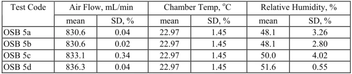
Uncertainty in Chamber Operation ConditionsSupply airflow rate, chamber temperature, and exhaust air humidity were carefully controlled and continuously monitored for all tests. The mean and % standard deviations of these
parameters observed for tests OSB5a, b, c, and d are summarized in Table 3. The highest observed environmental uncertainty was in the control of relative humidity with a relative standard deviation of 4%, equal to a deviation of only 2% RH units from the target value. Table 3: Chamber environmental conditions.
Air Flow, mL/min Chamber Temp, oC Relative Humidity, %
Test Code
mean SD, % mean SD, % mean SD, %
OSB 5a 830.6 0.04 22.97 1.45 48.1 3.26
OSB 5b 830.6 0.02 22.97 1.45 48.1 2.80
OSB 5c 833.1 0.34 22.97 1.45 50.0 4.02
OSB 5d 836.3 0.04 22.97 1.45 51.6 0.55
Uncertainty analysis for GC/MS measurements
Table 4 provides the calculated relative uncertainty (Ur) for several routinely calibrated VOCs.
The uncertainty from the relative response factor (Rct) dominates the overall uncertainty caused
by experimental error including analytical error with GC/MS. The uncertainty level is compound-specific, ranging from ~ 13 to 35%.
Table 4. Relative uncertainty for several target compounds analyzed by GC/MS. Class Compound ct R R ct σ (%) Ur (%) Class Compound ct R R ct σ (%) Ur (%) Hexane 15.38 18.38 Benzene 14.81 17.90
Heptane 7.89 12.78 Benzene, 1,4-dimethyl 10.42 14.47
Octane 16.35 19.19 Benzene, 1,2-dimethyl 17.89 20.52
Nonane 19.23 21.70 Ethyl benzene 11.21 15.05
Undecane 16.00 18.89 Styrene 8.86 13.40 Dodecane 13.98 17.22 Naphthalene 9.32 13.70 Alip ha tics Tetradecane 20.00 22.38 Aro m atics Benzene, 1,2,4-trimethyl 22.00 24.19 Butanal 17.65 20.31 α-Pinene 33.33 34.82 Pentanal 16.67 19.46 Camphene 19.23 21.70 Hexanal 20.00 22.38 3-Carene 15.22 18.24 Heptanal 14.29 17.47 Limonene 16.67 19.46 Nonanal 18.18 20.77 Al dehydes Decanal 19.05 21.54 Terpenes
Uncertainty analysis for HPLC measurements
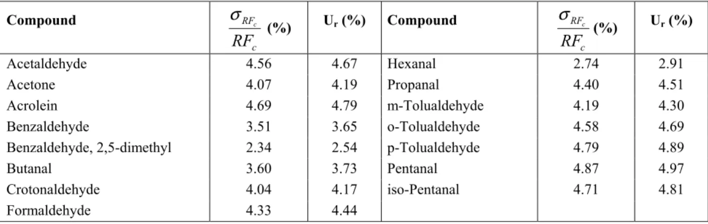
Table 5 summarizes the overall uncertainty associated with emission factors of compounds analyzed by HPLC. The uncertainty from the individual response factor (RFc) dominates the
uncertainty associated with experimental error with HPLC. In contrast to GC/MS analysis, which attempts to identify (and quantify) as broad a range of compounds as possible, the HPLC
analysis performed here targets carbonyl compounds only. This analytical focus is reflected in the relative improvement of the calculated uncertainties (ranging from about 2.5 to 5%) and highlights the importance of proper selection of analytical methods for the quantification of VOC emissions.
Table 5. Relative uncertainty for compounds analyzed by HPLC.
Compound c RF RF c σ (%) Ur (%) Compound c RF RF c σ (%) Ur (%) Acetaldehyde 4.56 4.67 Hexanal 2.74 2.91 Acetone 4.07 4.19 Propanal 4.40 4.51 Acrolein 4.69 4.79 m-Tolualdehyde 4.19 4.30 Benzaldehyde 3.51 3.65 o-Tolualdehyde 4.58 4.69
Benzaldehyde, 2,5-dimethyl 2.34 2.54 p-Tolualdehyde 4.79 4.89
Butanal 3.60 3.73 Pentanal 4.87 4.97
Crotonaldehyde 4.04 4.17 iso-Pentanal 4.71 4.81
Emission Variability: Qualitative Analysis (GC/MS)
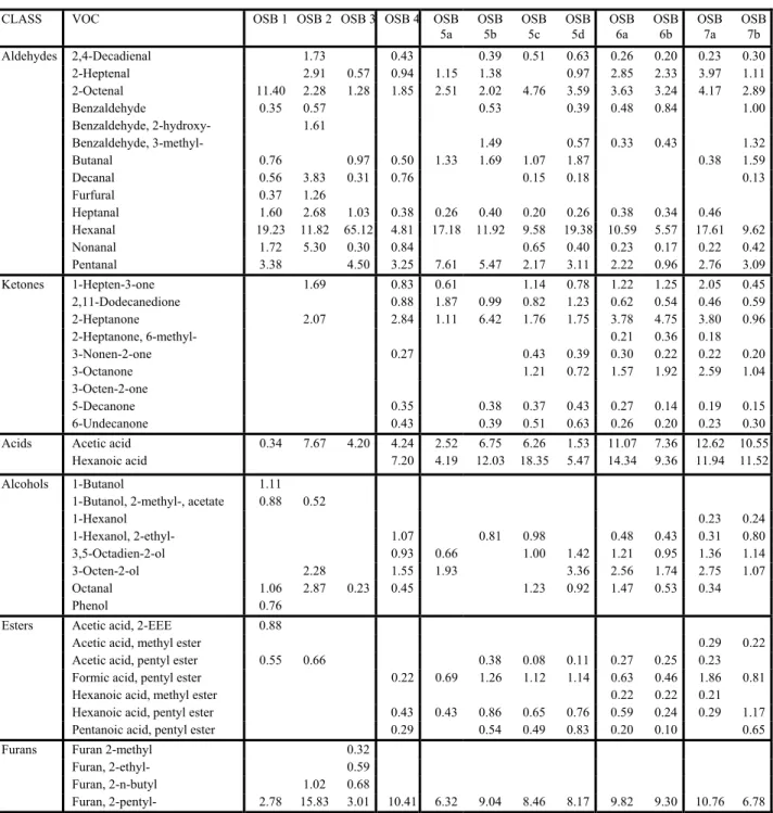
The results of the qualitative determination of all identifiable VOCs in the 24hr chamber samples are summarized by compound class in Table 6. Table 7 gives the complete analysis by
individual compounds. In general, the OSB specimens exhibited similarities in terms of the type of compounds emitted. Aldehydes, organic acids, 2-pentyl furan and α-pinene dominated the emission profiles. There are, however, some clear distinctions that can be made between the specimens based on this qualitative data.
Table 6. Summary of approximate VOC distributions (% of TVOC) at 24 hours by GC/MS.
VOC Class OSB 1 OSB 2 OSB 3 OSB 4 OSB 5a OSB 5b OSB 5c OSB 5d OSB6a OSB 6b OSB 7a OSB 7b Aldehydes 39.37 33.98 74.08 13.76 30.04 25.29 19.09 31.34 20.98 14.07 29.79 21.47 Ketones 3.75 5.59 3.59 8.19 6.25 5.93 8.23 9.37 9.72 3.70 Acids 0.34 7.67 4.20 11.44 6.71 18.78 24.61 6.99 25.41 16.73 24.56 22.07 Alcohols 3.82 5.68 0.23 4.00 2.59 0.81 3.22 5.69 5.71 3.65 4.99 3.25 Esters 1.43 0.66 0.93 1.12 3.05 2.33 2.84 1.90 1.27 2.88 2.85 Furans 2.78 16.84 4.60 10.41 6.32 9.04 8.46 8.17 9.82 9.30 10.76 6.78 Non-Aromatic Hydrocarbons 33.77 3.46 2.31 8.26 5.10 5.41 4.46 5.62 2.75 4.95 1.47 9.18 Aromatic Hydrocarbons 2.28 0.73 4.32 1.25 0.83 1.10 2.05 3.52 0.59 7.11 Chlorinated Hydrocarbons 0.78 1.80 1.18 0.49 0.14 7.74 0.20 5.04 Terpines 3.40 1.33 3.40 0.54 1.61 2.30 0.86 1.27 0.38 0.46 0.49 0.98 Total Identified VOCs (%): 87.96 73.36 89.56 61.06 57.09 74.10 71.29 69.44 77.38 71.04 85.43 82.42
Mill-mill variability is evident from review of the data from tests OSB1, 2, and 3. Non-aromatic hydrocarbons dominate OSB1 emission (many of these VOCs were only found with this
specimen). In contrast, the 2-pentyl furan content of OSB2 is relatively high, while aldehydes (particularly hexanal) dominate the emission from OSB3. OSB3 also exhibited a much broader range of furans than was observed with the other specimens. Ketones were not detected from OSB1 or OSB3, but were emitted in significant quantities from the remaining specimens (all from Mill B). The absence of detected hexanoic acid for tests 1, 2, and 3 may be due more to the switch to higher desorption and column temperatures in the later tests than to any compositional changes in the OSB specimens. The chlorinated hydrocarbon 1,4-dichloro benzene was detected in specimen OSB1 but not in OSB2 or 3. This compound showed interesting behavior in that significant quantities were detected in the emissions from specimens 6b and 7b, and lesser amounts from 5c, while the matched specimens for each of these tests (6a, 7a, and 5a,b,d) showed little or no emission of this VOC. Chamber background checks conducted prior to testing did not show the presence of this compound. Three separate chamber systems were used in tests 5c, 6b and 7a. It appears that this chemical in particular shows a high degree of
variability in emission level on a specimen-by-specimen basis even from the same test panel. Significant specimen-specimen variability was also observed in alcohol and organic acid
emissions in Tests 5a-d; and in hydrocarbon emission (both aromatic and non-aromatic) for tests 7a and 7b.
Table 7. Summary of approximate VOC concentrations (% of TVOC) at 24 hours by GC/MS.
CLASS VOC OSB 1 OSB 2 OSB 3 OSB 4 OSB
5a OSB 5b OSB 5c OSB 5d OSB 6a OSB 6b OSB 7a OSB 7b 2,4-Decadienal 1.73 0.43 0.39 0.51 0.63 0.26 0.20 0.23 0.30 2-Heptenal 2.91 0.57 0.94 1.15 1.38 0.97 2.85 2.33 3.97 1.11 2-Octenal 11.40 2.28 1.28 1.85 2.51 2.02 4.76 3.59 3.63 3.24 4.17 2.89 Benzaldehyde 0.35 0.57 0.53 0.39 0.48 0.84 1.00 Benzaldehyde, 2-hydroxy- 1.61 Benzaldehyde, 3-methyl- 1.49 0.57 0.33 0.43 1.32 Butanal 0.76 0.97 0.50 1.33 1.69 1.07 1.87 0.38 1.59 Decanal 0.56 3.83 0.31 0.76 0.15 0.18 0.13 Furfural 0.37 1.26 Heptanal 1.60 2.68 1.03 0.38 0.26 0.40 0.20 0.26 0.38 0.34 0.46 Hexanal 19.23 11.82 65.12 4.81 17.18 11.92 9.58 19.38 10.59 5.57 17.61 9.62 Nonanal 1.72 5.30 0.30 0.84 0.65 0.40 0.23 0.17 0.22 0.42 Aldehydes Pentanal 3.38 4.50 3.25 7.61 5.47 2.17 3.11 2.22 0.96 2.76 3.09 1-Hepten-3-one 1.69 0.83 0.61 1.14 0.78 1.22 1.25 2.05 0.45 2,11-Dodecanedione 0.88 1.87 0.99 0.82 1.23 0.62 0.54 0.46 0.59 2-Heptanone 2.07 2.84 1.11 6.42 1.76 1.75 3.78 4.75 3.80 0.96 2-Heptanone, 6-methyl- 0.21 0.36 0.18 3-Nonen-2-one 0.27 0.43 0.39 0.30 0.22 0.22 0.20 3-Octanone 1.21 0.72 1.57 1.92 2.59 1.04 3-Octen-2-one 5-Decanone 0.35 0.38 0.37 0.43 0.27 0.14 0.19 0.15 Ketones 6-Undecanone 0.43 0.39 0.51 0.63 0.26 0.20 0.23 0.30 Acetic acid 0.34 7.67 4.20 4.24 2.52 6.75 6.26 1.53 11.07 7.36 12.62 10.55 Acids Hexanoic acid 7.20 4.19 12.03 18.35 5.47 14.34 9.36 11.94 11.52 1-Butanol 1.11
1-Butanol, 2-methyl-, acetate 0.88 0.52
1-Hexanol 0.23 0.24 1-Hexanol, 2-ethyl- 1.07 0.81 0.98 0.48 0.43 0.31 0.80 3,5-Octadien-2-ol 0.93 0.66 1.00 1.42 1.21 0.95 1.36 1.14 3-Octen-2-ol 2.28 1.55 1.93 3.36 2.56 1.74 2.75 1.07 Octanal 1.06 2.87 0.23 0.45 1.23 0.92 1.47 0.53 0.34 Alcohols Phenol 0.76
Acetic acid, 2-EEE 0.88
Acetic acid, methyl ester 0.29 0.22
Acetic acid, pentyl ester 0.55 0.66 0.38 0.08 0.11 0.27 0.25 0.23
Formic acid, pentyl ester 0.22 0.69 1.26 1.12 1.14 0.63 0.46 1.86 0.81
Hexanoic acid, methyl ester 0.22 0.22 0.21
Hexanoic acid, pentyl ester 0.43 0.43 0.86 0.65 0.76 0.59 0.24 0.29 1.17
Esters
Pentanoic acid, pentyl ester 0.29 0.54 0.49 0.83 0.20 0.10 0.65
Furan 2-methyl 0.32
Furan, 2-ethyl- 0.59
Furan, 2-n-butyl 1.02 0.68
Furans
Table 7 (continued). Summary of approx. VOC concentrations (% of TVOC) at 24h by GC/MS.
CLASS VOC OSB
1 OSB 2 OSB 3 OSB 4 OSB 5a OSB 5b OSB 5c OSB 5d OSB 6a OSB 6b OSB 7a OSB 7b 1-Heptene 0.22 0.81 0.67 0.38 0.12 0.16 0.21 0.36 1-Hexene 0.40 1-Pentene 0.35 0.71 0.56 0.49 0.71 0.08 0.48 0.26 C10H22 1.74 C11H24 2.38 C12H26 0.34 C9H20 0.91 Cyclopentane, methyl- 0.68 Decane 0.61 0.68 0.24 1.46 0.53 1.14 0.97 0.76 1.46 2.69 0.43 5.70 Decane, 2,6-dimethyl 0.85 Dodecane 0.45 0.87 0.31 Heptane, 2,4-dimethyl- 3.74 Heptane, 2-methyl- 0.96 Heptane, 4-ethyl- 0.85 Hexane 1.07 0.59 Nonane 2.45 0.58 1.41 0.54 0.30 0.43 0.74 0.39 0.38 Nonane, 2,6-dimethyl- 1.28 Nonane, 2-methyl- 0.56 Octane, 4-methyl- 0.56 Octane, 4-methyl- 2.52 Pentadecane 0.82 0.14 Pentane 12.5 1.02 1.08 3.28 1.50 1.19 2.82 0.26 0.53 0.23 1.37 Pentane, 2-methyl- 1.78 Tetradecane 1.51 Non-Ar om atic Hydr ocar bons Undecane 0.88 0.55 0.58 0.61 0.66 0.25 0.35 0.20 1.11 Benzene 0.74 0.42 0.27 0.39 0.43 0.40 0.06 0.26 0.61 Benzene, 1,3,5-trimethyl- 0.94 1.44 0.39 2.55 Benzene, 1,3-dimethyl- 0.78 2.70 0.42 0.11 0.25 0.44 0.12 0.20 0.61 Benzene, 1-ethyl-3-methyl- 0.46 0.72 1.12 Benzene, 1-methyl-3-(1-ME) 0.31 Benzene, propyl- 0.38 Aromatic Hydr ocar bons Toluene 0.76 1.34 0.43 0.29 0.44 0.14 0.99 1.84 Cl-HCs Benzene, 1,4-dichloro- 0.78 1.80 1.18 0.49 0.14 7.74 0.20 5.04 3-Carene 0.39 α-Pinene 2.33 1.33 1.70 0.54 1.61 2.30 0.86 1.27 0.38 0.46 0.49 0.98 β-Pinene 0.92 Terp in es Limonene 1.07 0.39
Emission Variability: Quantitative Analysis
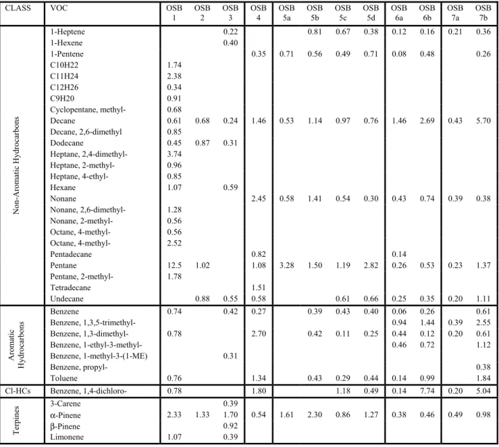
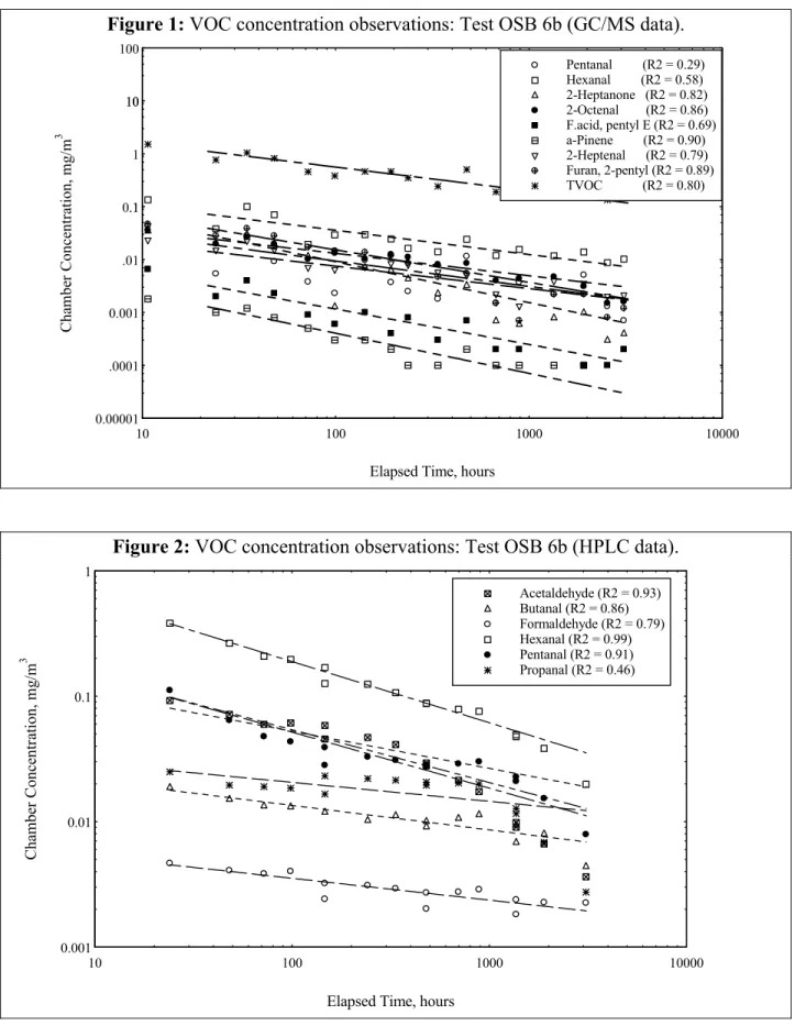
Examples of VOC chamber concentration data are given in Figure 1 (results from GC/MS samples) and Figure 2 (from HPLC analyses). The curves shown in these figures are the power law functions fitted to the experimental data. Correlation coefficients calculated for each VOC are indicated in the figure legends. The analytical variability as expressed by the correlation coefficients of the fitted curves was fairly typical in the example shown. VOCs quantified via GC/MS showed R2 values ranging from 0.29 (pentanal) to 0.90 for α-pinene. As described earlier, similar R2 values for HPLC analysis improved to between 0.46 (propanal) and 0.99 (hexanal). HPLC is obviously the method of choice for compounds such as hexanal and pentanal.
Figure 1: VOC concentration observations: Test OSB 6b (GC/MS data). 0.00001 0.001 0.1 10 .0001 .01 .1 1 10 100 10 100 1000 10000 Pentanal (R2 = 0.29) Hexanal (R2 = 0.58) 2-Heptanone (R2 = 0.82) 2-Octenal (R2 = 0.86) F.acid, pentyl E (R2 = 0.69) a-Pinene (R2 = 0.90) 2-Heptenal (R2 = 0.79) Furan, 2-pentyl (R2 = 0.89) TVOC (R2 = 0.80)
Elapsed Time, hours
Cha m be r C once ntra ti on, mg/m 3
Figure 2: VOC concentration observations: Test OSB 6b (HPLC data).
0.001 0.01 0.1 1 10 100 1000 10000 Acetaldehyde (R2 = 0.93) Butanal (R2 = 0.86) Formaldehyde (R2 = 0.79) Hexanal (R2 = 0.99) Pentanal (R2 = 0.91) Propanal (R2 = 0.46)
Elapsed Time, hours
Chamber Concen tr ation , m g/m 3
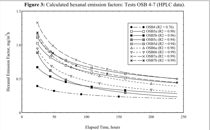
Examples of the modeled emission factors vs. time for hexanal (via HPLC) for tests 4 through 7 are shown in Figure 3 (the curve symbols in this plot are merely provided to assist with
identification and do not represent data points). Note the broad range of calculated emission factors for this single compound from the OSB specimens tested.
Figure 3: Calculated hexanal emission factors: Tests OSB 4-7 (HPLC data).
0 0.5 1.0 1.5 0 50 100 150 200 250 OSB4 (R2 = 0.76) OSB5a (R2 = 0.98) OSB5b (R2 = 0.96) OSB5c (R2 = 0.94) OSB5d (R2 = 0.94) OSB6a (R2 = 0.98) OSB6b (R2 = 0.99) OSB7a (R2 = 0.99) OSB7b (R2 = 0.99)
Elapsed Time, hours
H ex anal E m ission Facto r, mg/m 2 h
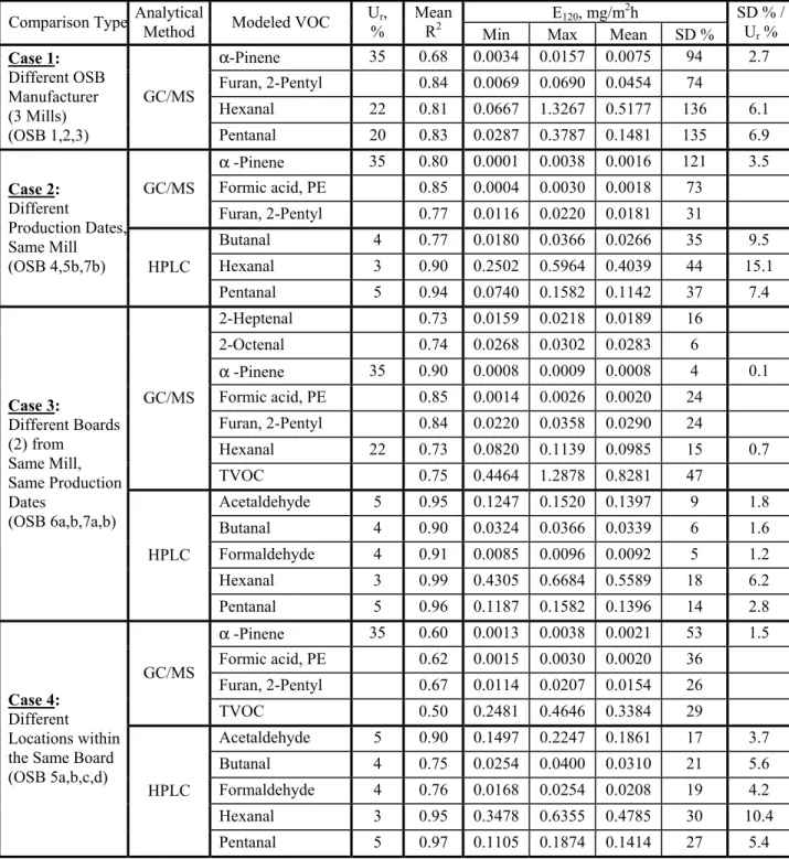
Table 8 summarizes the quantitative uncertainty analysis presented here. The test results are grouped vertically by the comparison made. For example, the first row in the table looks at mill-mill variability as revealed from tests OSB 1, 2 and 3. For each group of tests, representative VOCs were picked with relatively high R2 values from the concentration vs. time power fits. No point looking for specimen variability with noisy analytical data – this reflects the reality that not all compounds can be reliably quantified with the particular combination of sample tube,
desorption apparatus, GC column and operating conditions selected to give broad detection capabilities. For each VOC, the emission factor was calculated at 120 hours for each of the test specimens involved. For example, pentanal emission factors calculated for OSB 1, 2 and 3 had a mean value of 0.148 mg/m2h with a relative standard deviation of 135%. With an analytical uncertainty of approximately 20%, the pentanal emission variability at 120 hours thus exceeded the analytical uncertainty by a factor of about 7 to 1.
Table 8: Summary of VOC Emissions Variability.
E120, mg/m2h
Comparison Type Analytical Method Modeled VOC Ur,
%
Mean R2
Min Max Mean SD %
SD % / Ur % α-Pinene 35 0.68 0.0034 0.0157 0.0075 94 2.7 Furan, 2-Pentyl 0.84 0.0069 0.0690 0.0454 74 Hexanal 22 0.81 0.0667 1.3267 0.5177 136 6.1 Case 1: Different OSB Manufacturer (3 Mills) (OSB 1,2,3) GC/MS Pentanal 20 0.83 0.0287 0.3787 0.1481 135 6.9 α -Pinene 35 0.80 0.0001 0.0038 0.0016 121 3.5 Formic acid, PE 0.85 0.0004 0.0030 0.0018 73 GC/MS Furan, 2-Pentyl 0.77 0.0116 0.0220 0.0181 31 Butanal 4 0.77 0.0180 0.0366 0.0266 35 9.5 Hexanal 3 0.90 0.2502 0.5964 0.4039 44 15.1 Case 2: Different Production Dates, Same Mill (OSB 4,5b,7b) HPLC Pentanal 5 0.94 0.0740 0.1582 0.1142 37 7.4 2-Heptenal 0.73 0.0159 0.0218 0.0189 16 2-Octenal 0.74 0.0268 0.0302 0.0283 6 α -Pinene 35 0.90 0.0008 0.0009 0.0008 4 0.1 Formic acid, PE 0.85 0.0014 0.0026 0.0020 24 Furan, 2-Pentyl 0.84 0.0220 0.0358 0.0290 24 Hexanal 22 0.73 0.0820 0.1139 0.0985 15 0.7 GC/MS TVOC 0.75 0.4464 1.2878 0.8281 47 Acetaldehyde 5 0.95 0.1247 0.1520 0.1397 9 1.8 Butanal 4 0.90 0.0324 0.0366 0.0339 6 1.6 Formaldehyde 4 0.91 0.0085 0.0096 0.0092 5 1.2 Hexanal 3 0.99 0.4305 0.6684 0.5589 18 6.2 Case 3: Different Boards (2) from Same Mill, Same Production Dates (OSB 6a,b,7a,b) HPLC Pentanal 5 0.96 0.1187 0.1582 0.1396 14 2.8 α -Pinene 35 0.60 0.0013 0.0038 0.0021 53 1.5 Formic acid, PE 0.62 0.0015 0.0030 0.0020 36 Furan, 2-Pentyl 0.67 0.0114 0.0207 0.0154 26 GC/MS TVOC 0.50 0.2481 0.4646 0.3384 29 Acetaldehyde 5 0.90 0.1497 0.2247 0.1861 17 3.7 Butanal 4 0.75 0.0254 0.0400 0.0310 21 5.6 Formaldehyde 4 0.76 0.0168 0.0254 0.0208 19 4.2 Hexanal 3 0.95 0.3478 0.6355 0.4785 30 10.4 Case 4: Different Locations within the Same Board (OSB 5a,b,c,d)
HPLC
Pentanal 5 0.97 0.1105 0.1874 0.1414 27 5.4
Using the same comparative approach, Table 8 indicates a slightly higher degree of variability for Case 2 (same mill, different production dates): the ratio of uncertainties (SD %/ Ur %)for α
-pinene equals 3.5 vs. 2.7 for Case1. While formaldehyde emission from boards produced on the same date by the same mill (Case 3) was relatively consistent, hexanal and pentanal emission showed a greater degree of variability (HPLC data). This trend was not observed with the
GC/MS data for hexanal, however, likely due to its higher analytical uncertainty for this
compound. In Case 4 (multiple samples from the same board), hexanal emission exhibited even higher variability.
CONCLUSIONS
A series of tests of OSB were conducted to examine the degree of variability that can occur in the emissions of VOCs from a single building product. While the sample size is small, and limits detailed statistical analysis, some observations of interest were found.
Experimental uncertainty with the GC/MS was found to be strongly compound-specific, with a mean value of about 19% (ranging from ~12% to ~35%). HPLC uncertainty, for a much narrower spectrum of VOCs, and a system optimized for their collection and analysis, was not surprisingly much lower at about 4.2 % (2.5 to 5% range).
In the analysis of OSB emissions variability, mill-mill differences were evident (qualitatively and quantitatively), as were differences between production dates, between individual panels with the same production date, and even between specimens taken from a single panel.
In summary, variability inherent within the building material itself should be considered when comparing different building material options (as in labeling schemes) or in the development and validation through chamber testing of models for VOC emission. Variability assessment should be conducted while keeping in mind appropriate selection of target VOCs and analytical
methods so as to minimize analytical error that could otherwise mask variability. Round robin certification of test labs should consider these factors and design their comparisons accordingly. Precise definition and control of emission testing protocols is essential, but not the complete answer to emissions standardization.
ACKNOWLEDGMENTS
The authors would like to acknowledge Gang Nong, Institute for Research in Construction, National Research Council of Canada, and Sara Yonson, student: McMaster University for their technical assistance with the dynamic chamber tests. Financial support from the Consortium for Material Emission and IAQ Modeling, NRCC is gratefully acknowledged.
REFERENCES
1. Yu, C.; Crump, D., Building and Environment, 1998, 33 (6), 357-374.
2. Kukkonen, E.; Saarela, K.; Neuvonen, P. In Proc. Indoor Air 2002, 9th Int'l Conf. On IAQ and Climate, Monterey, Calif, June 30 - July 5, 2002, Vol.3, 588-592.
3. Oppl, R. In Proc. Indoor Air '99, 8th Int'l Conf. On IAQ and Climate, Edinburgh, Scotland, Aug.8-13, 1999, Vol.1, 543-548.
4. Witterseh, T. In Proc. Indoor Air 2002, 9th Int'l Conf. On IAQ and Climate, Monterey, Calif, June 30 - July 5, 2002 Vol.3 612-614.
5. Bluyssen, P.M.; Fernandes, E. de Oliveira , Molina, J.L. (2000), In Proc. Healthy Buildings, Vol.2, 385-390, 2000.
6. Canilli, C.; Johnston, P.; Koontz, M.D.; Girman, J.R.; Kennedy, P.W. (1993), in Proc. Indoor Air '93, Vol.2, 425-430.
7. Clausen, G, de Oliveira Fernandes, E, Fanger, PO, (1996), in Proc. Indoor Air '96, Vol.2, 639-644.
8. Zhang, J.S.; Shaw, C.Y.; Sander, D.; Zhu, J.P.; Huang, Y. MEDB-IAQ: A material emission database and single-zone IAQ simulation program - A tool for building designers, engineers and managers. Consortium for Material Emissions and Indoor Air Quality Modeling
(CMEIAQ), Final Report 4.2, Institute for Research in Construction, NRCC, 1999.
9. Levin, H.; Hodgson, A.T., In Characterizing sources of indoor air pollution and related sink effects, ASTM-Special-Technical-Publication. n 1287, 376-391, 1996.
10. ASTM, D5116 - Standard Guide for Small-Scale Environmental Chamber Determinations of Organic Emissions From Indoor Materials/Products, American Society for Testing and Materials, 1997.
11. CEN Building products - determination of the emission of volatile organic compounds. Part 1: Emission test chamber method; Part 2: Emission Cell Method; Part 3: Procedure for sampling, specimen preparation and preconditioning of materials and products. ENV Pr13419, 1998.
12. Larsen, A. Consensus meeting on chemical testing of emission from building products. Nordtest Report TR 506, 2002.
13. Magee, R.J.; Zhu, J.P.; Zhang, J.S.; Shaw, C.Y. A Small Chamber Test Method for Measuring Volatile Organic Compound Emissions from "Dry" Building Materials.
Consortium for Material Emissions and IAQ Modeling (CMEIAQ) Final Report 1.2, Institute for Research in Construction, NRCC, 1999
14. Saarela, K.; et al Emission classification of building materials: Protocol for chemical and sensory testing of building materials, The Building Information Foundation RTS (ISBN 951-682-673-3) 2002.
15. Wolkoff, P. The Science of the Total Environment, 1999, 227, 197-213.
16. Oppl, R.; Winkels, K., Proc. Indoor Air 2002, 9th Int'l Conf. On IAQ and Climate, 2002, Vol.2,902-907.
17. deBortoli, M; et al, Indoor Air, 1999, 9, 103-116.
18. Hansen V.; Larsen A.; Wolkoff, P., In Proc. Healthy Buildings '00, 2000, Vol.4, 99-101. 19. Barry, A.O.; Corneau, D., Holzforschung 1999, 53 (4), 441-446.
20. Zhu, J.P.; Lusztyk, E., Zhang, J.S., Shaw, C.Y. A Method for Sampling and Analysis of Volatile Organic Compounds in Emission Testing of Building. Consortium for Material Emission and IAQ Modeling (CMEIAQ), Final Report 1.1, 1999.
21. Yang, X.; Chen, Q.; Zhang, J.S.; Magee, R.J.; Zeng, J.; Shaw, C.Y. Building and Environment 2001, 36 (10), 1099 –1107.
22. Zhu, J.; Magee, R.J.; Zhang, J.S.; Lusztyk, E.; Shaw, C.Y., Air & Waste Management Association's 1999 Annual Meeting and Exhibition, 1999, 1-14.
23. Zhu, J.; Zhang, J.S.; Lusztyk, E.; Magee, R.J. Air & Waste Management Association 91st Annual Meeting & Exhibition, 1998, 1-16.
24. Zhu, J.; Zhang, J.S.; Shaw, C.Y., Chemosphere 2001, 44, 1253-1257.
Key Words
• material emissions
• oriented strand board
• chamber testing
• VOC
• Volatile organic compounds
• Variability