Analysis and design of wave scattering by weakly non-uniform waveguides

Analysis and Design of Wave Scattering by

Weakly Non-uniform Waveguides.

by

Karl Peter Burr

Submitted to the Department of Ocean Engineering

in partial fulfillment of the requirements for the degree of

Doctor of Philosophy in Hydrodynamics

at the

MASSACHUSETTS INSTITUTE OF TECHNOLOGY

September 2001

Karl Peter Burr, MMI. All rights reserved.

The author hereby grants to MIT permission to reproduce and

distribute publicly paper and electronic copies of this thesis document

in whole or in part.

A uthor ...

...

...

Department of Ocean Engineering

September 6, 2001

C ertified by ...

...

Dick K. P. Yue

Professor of Hydrodynamics and Ocean Engineering

A

The-.supervisor

Certified by...

Accepted by...

Michael S.

iantafyllou

Profe

an Engineering

'tdesis Supervisor

Henrik Schmidt

Professor of Ocean Engineering

Chairman, Department Committee on Graduate Students

MASSACHUSETTS IN TITUT OF TECHNOLOGY

NOV 2 7 2001

UIBRARIES

Analysis and Design of Wave Scattering by Weakly

Non-uniform Waveguides.

by

Karl Peter Burr

Submitted to the Department of Ocean Engineering on September 6, 2001, in partial fulfillment of the

requirements for the degree of Doctor of Philosophy in Hydrodynamics

Abstract

When waves propagate through a medium with small irregularities of the size of the order of many wavelengths, a number of interesting phenomena may happen such as wave localization and large sensitivity of the wave field behavior with respect to the medium irregularity variation. These phenomena occur due to the interaction of the incident wave field with the medium small irregularities, and open the possibility of designing the system irregularity to achieve a desired vibratory response. This has a variety of engineering applications, such as the the design of the sea bottom of coastal areas to provide protection against the incoming swells, or the design of the material and geometrical properties of the cross section of pipelines, risers and mooring lines such that vibration transmission is minimized.

The objective of this thesis is to understand how to tune the medium small irregu-larity such that the interaction of the incident wave field with the medium irreguirregu-larity generates a desired reflected wave field. A particular design problem of interest is the prediction of the minimum amount of changes in the medium irregularity needed to minimize wave transmission to a desired level for a given range of frequencies of interest.

As a model problem, we considered disordered chains of repetitive systems with the size of the order of many wavelengths of the incident wave. We applied an asymptotic theory for wave propagation along the non-uniform chain. For weak coupling between subsystems, the asymptotic theory predicted new results, such as exponential small transmission due to wave tunneling and explained localization phenomena as a turning point problem. For strong coupling, the asymptotic theory provided fundamental understanding of the effects of the irregularity on wave propagation.

Pipelines and risers can be modeled as slender beams under tensile force. To describe well the effects of small irregularity in beams vibration, we derived asymp-totically a simpler governing equation for the vibration problem. This new equation is asymptotic with respect to the beam irregularity steepness, but under the restriction of constant product of the flexural rigidity by the mass per unit length and constant tensile force, this new equation is an exact equation for the beam vibration and has

A -w ,

a Helmholtz-like form. Inverse scattering methods for the Helmholtz-like equations

can be applied to design the beam non-uniformity such that desired wave scattering

properties are achieved. We also constructed a high order asymptotic solution for

the scattering of mono-chromatic waves by the irregularity in slender beams. The

asymptotic method used is the WKB method, which is basically a wave refraction

theory, but we improved it such that wave reflection and wave mode conversion were

captured.

The asymptotic approach developed in the previous problems is extended and

applied to the interaction of linear surface gravity waves with a bottom topography

which varies slowly with respect to the length scale of the incident wave field. The

asymptotic theory captured wave reflection and transmission and wave mode

con-version, which leads to a more complete asymptotic representation of the wave field.

This asymptotic theory also reveals the dependence of the scattering coefficients with

respect to the bottom geometry, which is a fundamental step in the design of bottom

topographies in coastal areas to provide protection against the incoming swells.

Thesis Supervisor: Dick K. P. Yue

Title: Professor of Hydrodynamics and Ocean Engineering

Thesis Supervisor: Michael S. Triantafyllou

Title: Professor Ocean Engineering

Acknowledgments

I wish to express my sincere appreciation and gratitude to my advisors, Professor Yue and Professor Triantafyllou for their guidance, discussions and suggestions in all stages of my thesis work and for their financial support during part of my stay as student at MIT. I also wish to thank the members of my thesis committee, Professor Scalvounos, Professor Makris and Professor Akylas for their suggestions and patience in reviewing this thesis.

I wish to thank Professor Akylas for our discussions and his suggestions in the final stages of my thesis work, and for the opportunity to work with him as teaching assistant in the the Fall of 2000, and in the Spring and Summer of 2001.

I gratefully acknowlege the financial support for my initial three and a half years at MIT from CNPq-Conselho Nacional Cientifico e Tecnol6gico, of the Ministry for Science and Technology of Brazil under grant 201378/92-2(RN).

I also wish to express my appreciation to my friends Drausio Giacomelli, Leandro Farina, Luiz Lopez Souza, Antonio Makiyama and Michele Zanolin, for their friend-ship in the difficult moments during my stay at MIT. I also wish to thank my research group for their help, specially in the final stages of my thesis work.

Contents

2 Asymptotic Analysis of Wave Propagation along Weakly Non-uniform Repetitive Systems. ₄₅

2.1 PREVIOUS WORK. . . . .

47

2.2 _{ONE-DIMENSIONAL CHAIN OF COUPLED PENDULA. . . . . . 48}

2.3 _{THE WKB METHOD FOR SECOND ORDER DIFFERENCE} EQUA-TIO N S. .. . . . .. 51

2.3.1 LIOUVILLE-GREEN FUNCTIONS... 51

2.3.2 TURNING POINT CONDITIONS... 56

2.3.3 APPROXIMATE EQUATIONS. ... 59

2.3.4 CONNECTION FORMULAE... 62

2.3.5 ASYMPTOTIC FORM OF THE SYSTEM TRANSFER MA-TRIX.. ... 70

2.4 APPLICATION... .. ... 74

2.4.1 _{SYSTEM WITH ONE PAIR OF TURNING POINTS. ... 74}

2.4.2

SYSTEMS WITH TWO PAIRS OF TURNING POINTS.

78

2.5

DISCUSSION AND CONCLUSIONS. ...

82

3 Asymptotic Analysis and Design of Wave Propagation Along a Non-Uniform Euler-Bernoulli Beam. 85 3.1 Asymptotic Governing Equation for Wave Propagation along Weakly Non-uniform Euler-Bernoulli Beams. ... ... 87

3.1.1 Previous Work. ... 89

3.1.2 Bernoulli-Euler Beam Governing Equation. . . . 90

3.1.3 Second Order Governing Equation for the Bernoulli-Euler Beam. 93 3.1.4 Applications - The Analysis Problem. . . . 109

3.1.5 Applications - The Design Problem. . . . . 123

3.1.6 Discussion and Conclusions. . . . . 127

3.2 High Order WKB Method for the Euler-Bernoulli Beam. . . . . 130

3.2.1 Euler-Bernoulli Beam Governing Equation Revisited. . . . . . 133

3.2.2 High Order Liouville-Green Functions. . . . . 134

3.2.3 Turning Points of the Operator L . . . . 144

3.2.4 Approximate form of the Beam Equation for a Neighborhood of a First Order Turning Point. . . . . 167

3.2.5 Matching Process. . . . . 209

3.2.6 Global Reflection and Transmission Coefficients . . . . 243

3.2.7 Discussions and Conclusions . . . . 245

4 Interaction of Linear Surface Gravity Waves with a Weakly Non-uniform Bottom Topography. 250 4.1 _{Previous W ork. . . . . 252}

4.2 Chapter Overview. . . . . 254

4.3 Linear Surface Gravity Waves Boundary Value Problem. . . . . 257

4.4 Operator Method Approach for Linear Surface Gravity Waves. . . . . 261

4.5 Asymptotic Solution Through a High Order WKB Approach.. . . . . 266

4.5.1 The Eikonal Equation and the Transport Equation. . . . . 267

4.5.3 Approximate Equations for the Free Surface Potential. . . . . 300

4.5.4 Matching Process at a Turning Point. . . . . 327

4.5.5 Local Transfer Matrix. . . . . 359

4.6 Global Transfer Matrix. . . . . 366

4.7 Discussion and Conclusions. . . . . 368

5 Summary and Future Work. 371 A HIGH ORDER WKB METHOD FOR SYSTEMS OF FIRST OR-DER DIFFERENCE EQUATIONS. 382 A.1 Reduction of first order difference equations to a recurrence relation.. 383

A.2 High order Liouville-Green functions for a high order difference equation. 393 A.3 Turning Points. . . . . 397

A.4 Difference Equations as Pseudo Differential Equations. . . . . 401

B PROCEDURE TO OBTAIN THE TURNING POINTS OF

Q.

C.1 CONNECTION FORMULAE FOR A PAIR OF COMPLEX FIRST

C.1.1 Leading Term of the Asymptotic Expansion of the Functions Hg(?,v)... ... ... 407

C.1.2 LOCAL APPROXIMATION OF THE LIOUVILLE-GREEN FORM ULA... . 419

C.1.3 MATCHING PROCESS... 423

C.2 CONNECTION FORMULAE FOR A PAIR OF ALMOST

C.2.2 ASYMPTOTIC EXPANSION OF THE SOLUTION OF THE APPROXIMATE EQUATION. ... 429

C.2.3 MATCHING PROCESS FOR A PAIR OF ALMOST

COA-LESCING COMPLEX CONJUGATE FIRST ORDER

TURN-ING POINTS. ... 430

C.2.4 MATCHING PROCESS FOR A PAIR OF ALMOST

COA-LESCING REAL FIRST ORDER TURNING POINTS. . . . 431 D Governing Equation for Quantities A(s), B(s), C(s) and D(s) and

Ele-ments of the matrix M(s). 433

E Order of Magnitude of the Elements of Matrix M(s). 437 E.1 RegimeO +0..-+. ... 437 E.2 Regime 0> 1.... ... 440

F Decoupling of the Propagating and Evanescent Part of the

Wave-field. 443

G Second Order Equation with Analytic Solution. 445

H Reflection and Transmission Coefficients for The Bernoulli-Euler

Beam. 447

I Outline of the Steepest Descent Method. 451

1.1 Asymptotic Expansion of the Functions H1

(6,

J Recurrence Relations for the Symbols A" (x, p) and B (x, p). 455

K Expression for the Symbols L(x, p). 466

L Derivation of the Transport Equations. 469

M Local Form of the Liouville-Green functions. 490

M.1 Approximate Liouville-Green Functions for Turning Points where a Propagating and an Evanescent Wave Modes Couple. ... 492

M.2 Approximate Liouville-Green Functions for Turning Points where the two a Propagating Wave Modes Couple. . . . 498

List of Figures

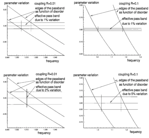
1-1 A two degree of freedom chain of coupled pendulums. . . . . 29 2-1 Examples of effective pass band for some values of the coupling

param-eter R and for some values of the range of the variation of the length of the pendula

(%)

j=1,..

Stokes lines ---

--

)

<j

(pair

j*i,,

j

and j*1,-2, details box (B)). TPP3: a 1 <

j

coalescent complex conjugate turning points J*2,e+1 and 1*2,1+1). TPP4

a 1 < j < a1+ 2 (pair of almost coalescent real turning points j,1,1+2

and J71,1+2). TPP5: a, 1 <

j

(second

2-3 Modulus of the Reflection coefficient for left incidence. We have a second order turning point at 30% of the uniform system passband. The turning points satisfy the first turning point condition. Amplitude A = 0.012. Coupling parameter is R = 0.01. The full line denotes the numerical results. The ... line denotes the usual WKB approximation.

The - - -- line denotes the reflection coefficient given by (2.61) and

(2.63).The - - - line denotes a composite approximation. For

frequencies close to the frequency for which we have a second order turning point, the reflection coefficient is given by (2.61) and (2.63).

Otherwise, it is given by (2.49) and (2.57). . . . . 76

2-4 Modulus of the transmission coefficient for left incidence. We have a second order turning point at 70% of the uniform system passband. The turning points satisfy the second turning point condition. Am-plitude A = 0.012. Coupling parameter is R = 0.01. The full line

denotes the numerical results. The . . . line denotes the usual WKB

approximation. The - - -- line denotes the transmission coefficient given by (2.64).The - - -- --- line denotes a composite approximation. For frequencies close to the frequency for which we have a second order turning point, the transmission coefficient is given by (2.64).

Other-wise, it is given by (2.52) and (2.60). . . . . 77 2-5 _{Modulus of the Reflection coefficient for left incidence. We have a}

second order turning point at 30% of the uniform system passband. The turning points satisfy the first turning point condition. Amplitude

A = 0.012. Coupling parameter is R = 0.01. The full line denotes the

numerical results. The - - - - _{line denotes the reflection coefficient} given by (2.61) and (2.63).The - - -- line denotes given by (2.49) and (2.57). . . . . 78

2-6

Modulus of the Reflection coefficient for left incidence. We have a

second order turning point at 25% and 75% of the uniform system

passband. Amplitude A

=

0.0098. Coupling parameter is R

= 0.01.

The full line denotes the numerical results. The - - -- line denotes

the reflection coefficient given by the transfer matrix method. We use

the local reflection/transmission coefficients given by the usual WKB

transmis-sion coefficients corrected by the approximation for almost coalescing

pairs of turning points problem. We use this correction when the wave

frequency is close to the frequency for which the turning point problem

is a second order real turning point. . . . .

80

2-7 Modulus of the Transmission coefficient for left incidence. We have

a second order turning point at 25% and 75% of the uniform system

passband. Amplitude A = 0.0098. Coupling parameter is R = 0.01.

de-notes the transmission coefficient given by the transfer matrix method.

We use the local reflection/transmission coefficients given by the usual

transmission coefficients corrected by the approximation for almost

co-alescing pairs of turning points. We use this correction when the wave

frequency is close to the frequency for which the turning point problem

is of second order... . ..

. . .

...

. . ...

81

3-1 Reflection coefficient as a function of wave frequency of the incident wave. JRI: modulus of the reflection coefficient. A RJ: difference between modulus of the reflection coefficient. Vertical arrows: Bragg scattering peaks. In parts

(a)

(c),

- - _{: numerical simulation of the full governing equation (3.6),} respectively, for A/ho = 0.2, 0.1 and 0.05, and lines..., ---

and

-.--- _{: numerical simulation of the second order governing equation} (3.49) for A/ho = 0.2, 0.1 and 0.05. In parts (b) and (d), lines

, - - - and - - -- : difference between modulus of the reflection coefficient, respectively, for A/ho = 0.2, 0.1 and 0.05. . . . . 115 3-2 Reflection coefficients as a function of wave frequency of the incident

wave. JRI: modulus of the reflection coefficient. A RI: difference between modulus of the reflection coefficient. Vertical arrows: Bragg scattering peaks. In parts

(a)

(c),

(3.6),

respectively, for A/ho = 0.1, 0.05 and 0.01, and lines...,

-and ---

:

equation (3.49), respectively, for A/ho = 0.1, 0.05 and 0.01. In parts

(b)

(d),

modulus of the reflection coefficient, respectively, for A/ho = 0.1, 0.05 and 0.01. . . . 116

3-3 Modulus of the reflection coefficient as a function of wave frequency of the incident wave. In parts

(a)

(b),

-- -- _{: numerical simulation of the full governing equation (3.6) with}

A/ho, respectively, 0.05 and 0.01, and lines-...and

numerical simulation of the second order governing equation (3.49) with A/ho, respectively, 0,05 and 0.01. Part (c) displays contour plots for Q(s) = 0. The letters P and N in part (c) stands for positive and negative values of Q(s). Line--- : AO = 10000N, k= 10, k9 = 2

and A/ho=0.05, and line--- : Ap = 10000N,kc=10, kg = 2 and A

/ho

of the incident wave. Non-dimensional flexural rigidity and mass per unit length defined by equations (3.77) and (F.3), with C = 1, r = 20, k9 = 27r, so = 10.25 and

y

full governing equation (3.6) with A, respectively, equals to 0.2, 0.1

and 0.05. Lines-..., --- and : numerical simulation of

the second order governing equation (3.49) with A, respectively, equals to 0.2, 0.1 and 0.05. . . . . 121

3-5 Modulus of the reflection coefficient as a function of wave frequency of the incident wave. Non-dimensional flexural rigidity and mass per unit

length defined by equations (3.78) and (F.3) with C = 1. Lines ---and-...: numerical simulation of the full governing equation (3.6).

Symbols LI and A: Closed form solution given by equations (3.78) and

(3.81). Line --- and symbol El: kg = 10. Line...and symbol A: k9 = 5. Values of the parameters S, N, M and so and the tensile

force P for parts (a), (b), (c) and (d) are listed in table 3.3. In part (e), lines and - - - -: non-dimensional flexural rigidity distribution used in parts (a) and (b) with kg, respectively, equals to 10 and 5 , and lines --- and...: non-dimensional flexural rigidity

distribution used in parts (c) and (d) with kg, respectively, equals to

10 and 5.. . . . ... 122 3-6 Modulus of the reflection and transmission coefficients as a function

of wave length of the incident wave for the designed Euler-Bernoulli beam. f-l from equation (3.93): - - - --. iT- = 1 - R -12:

...-.-.

Numerical simulation for the reflection coefficient (H.13): El. Numerical results for the transmission coefficient (H.13): A. Proper-ties of the designed beams for (a), (b), (c) and (d) are given in table

(3.5). . . . . 12 8 3-7 Turning points for non-uniformity in the flexural rigidity. Tensile load

equals to 1000 N. Wave frequency: (a) - 2 Hz, (b) - 10 Hz, (c) -20 Hz and (d) - 30 Hz. The symbols representing the position of the

turning points are associated with the non-uniformity non-dimensional

amplitude. Symbols: H - A = 0.01, A - A = 0.1, V - A = 0.2. . . . . 155 3-8 Turning points for non-uniformity in the flexural rigidity. Tensile load

equals to 10,000 N. Wave frequency: (a) - 2 Hz, (b) - 10 Hz, (c) -50 Hz and (d) - 90 Hz. The symbols representing the position of the

turning points are associated with the non-uniformity non-dimensional

3-9 Examples of the two types of contours in the z plane. Arrows indicates in which sense we travel along the contours. (a) - contour of the first type. (b) - _{contour of the second kind. Tensile load P = 10,000 N.}

The wave frequency for (a) is 2 Hz, which gives turning points further apart of each other. In (b) the wave frequency is 10 Hz. . . . 161 3-10 Continuum of numerical values that the wave numbers dS/dz assume

as the contour in part (a) of Figure (3-9) encircles chosen turning points. Arrows indicate in which sense the wave numbers evolve as we encircle a turning point. Tensile load P = 10,000 N and wave

fre-quency is 2 Hz. (a) - 1 st chosen turning point . (b) - 2 nd chosen turning point. (c) -3 rd chosen turning point. (d) - 4 th chosen turning point. Line - numerical value of dS1

/dz.

-numerical value of dS2

/dz.

/dz.

Line-... - numerical value of dS4

/dz.

3-11 Continuum of numerical values the wave numbers dSg/dz assume as

the contour in part (b) of Figure (3-9) encircles chosen pairs of turning points. Arrows indicates in which sense the wave numbers evolve as we encircle a pair of turning points. Tensile load P = 10,000 N and

wave frequency is 10 Hz. (a) - 1 st chosen pair of turning points .

(b)

/dz.

-numerical value of dS3

/dz.

/dz.

3-12 Continuum of numerical values assumed by the wave numbers dSI/dz (part (a)) and dS2

/dz

j

1,... , 3 and the rays r₁, r2 and r3 specified, respectively, by equations

(3.198), (3.199) and (3.197). The arrows in the integration contours

Aj indicate the way we travel along the contours as the integration is

3-14 Sketch of the sectors SRj in the complex z plane. The range of arg{z} for these sectors is given by equations (3.206) to (3.208) with n = 0. 173 3-15 A sketch in the complex t plane of the integration contours A,,

j

4, 5,6 and 1 = 1,2, 3, of the rays ri, r2 and r3 and of the rays R1, R2 and

R3 specified, respectively, by equations (3.203), (3.204) and (3.205). The arrows in the integration contours Aj1 indicate the way we travel

along the contours as the integration is performed. The half plane where the contour end point condition is satisfied as tI -+ oc is given

by the position of the shadow with respect to the line crossing the

origin. If the shadow is above (below) the line, the contour end point condition is satisfied for It|

<

3-16 A sketch in the complex t plane of the closed integration contours

used to continue the solution A1,, defined in the sector SR2 (SR3) for -wr </# < 0 (0 </3 <w-r) by the integration contour A422 (A43) to the sectors SR3 (SR2) and SR1. . . . 177

3-17 Stokes lines for the approximate equation (3.188) with

/2

quadrant (bounded by the bottom and right going lines DS1 3), region

Sio (S4) - 3rd quadrant (bounded by the bottom and left going lines

DS1 3) and region S9 (S3) - 2nd quadrant (bounded by the left going

line DS13 and the branch-cut). At the 2nd (4th) Riemann sheet (top (bottom) right figure): Region S3 (S9) - 1st quadrant, region S2 (S8)

-4th quadrant, region Si (S7) - 3rd quadrant and region So (S6) - 2nd

quadrant. Notice that for this Riemann sheet, regions are bounded by lines DS14 (DS14) and branch-cuts. . . . . 195

3-18 Stokes lines for the approximate equation (3.188) with / = -i. These

3.'

lines are defined according to equation (3.246). At the 1st (3rd) Rie-mann sheet (top (bottom) left figure): Region So (Se) - 1st quadrant (bounded by branch-cut and right line DS13), region S11 (S₅) - 4th quadrant (bounded by the bottom and right going lines DS13), region

Sio (S4) - 3rd quadrant (bounded by the bottom and left going lines

DS1 3) and region S9 (S3) - 2nd quadrant (bounded by the left going

line DS13 and the branch-cut). At the 2nd (4th) Riemann sheet (top

(bottom) right figure): Region S3 (59) - 1st quadrant, region S2 (S8) -4th quadrant, region Si

(S7)

lines are defined according to equation (3.246). At the 1st (3rd) Rie-mann sheet (top (bottom) left figure): Region So (Se) - 1st quadrant (bounded by the top and right going lines DS14), region S1 (S5) - 4th

quadrant (bounded by the branch-cut and the right going line DS14), region S2 (S8) - 3rd quadrant (bounded by the branch-cut and the left going lines DS14) and region Si (S7) - 2nd quadrant (bounded by the left and top going lines DS14). At the 2nd (4th) Riemann sheet (top (bottom) right figure): Region S3 (59) - 1st quadrant, region S2 (S8) -4th quadrant, region S5 (S11) - 3rd quadrant and region S4 (Sio) - 2nd quadrant. Notice that for this Riemann sheet, regions are bounded by lines DS13 (DS13) and branch-cuts. . . . 197

3-20 Stokes lines for the approximate equation (3.188) with = ,. _3. These lines are defined according to equation (3.246). At the 1st (3rd) Rie-mann sheet (top (bottom) left figure): Region So (Se) - 1st quadrant

(bounded by the top and right going lines DS13), region S11 (S5) - 4th

quadrant (bounded by the branch-cut and the right going line DS13),

region S2 (S8) - 3rd quadrant (bounded by the branch-cut and the left

going lines DS1 3) and region S1

(S7)

left and top going lines DS1 3). At the 2nd (4th) Riemann sheet (top (bottom) right figure): Region S3 ( S) - 1st quadrant, region S2 (S8)

-4th quadrant, region S5 (S11) - 3rd quadrant and region S4 (Sio) - 2nd quadrant. Notice that for this Riemann sheet, regions are bounded by lines DS14 (DS14) and branch-cuts. . . . . 198

3-21 Sketch of turning points problems and points A, B, and C, in the

complex z plane for the non-uniformity in the flexural rigidity only,

and specified by equation (3.178). . . . . 210 3-22 Sketch of the integration contours Fo, IF0 1, F0 2, I, IF, and F1 2 in the

complex z plane for the non-uniformity in the flexural rigidity only,

and specified by equation (3.178). . . . . 232

4-1 Example of a one-dimensional non-uniform bottom topography. . . . 258

4-2 Enumerated branch points in the complex h plane. Branch point at

the origin not displayed. . . . . 275

4-3 Saddle points in the complex wavenumber k plane, which are images of the enumerated branch points in the complex h plane. . . . . 276

4-4 Some contour given by equation (4.86) in the complex h plane. . . . . 280

4-5 Trajectory of the wave numbers that coalesce at the two saddles, image of the first branch point, as we go along contour (4.86) with hb as the first branch point (m = 1). . . . . 282

4-6 Trajectory of the wave numbers that coalesce at the two saddles, image of the second branch point, as we go along contour (4.86) with h₆ as the second branch point (m = 1). . . . . 283

4-7 _{Trajectory of the wave numbers that coalesce at the two saddles, image} of the third branch point, as we go along contour (4.86) with h6 as the third branch point (m = 2). . . . . 284

4-8 _{Trajectory of the wave numbers that coalesce at the two saddles, image} of the fourth branch point, as we go along contour (4.86) with hb as

the fourth branch point (m = _{2). . . . 285} 4-9 Trajectory of the wave numbers that coalesce at the two saddles, image

of the fifth branch point, as we go along contour (4.86) with h, the fifth

branch point (m = _{3). . . . . 286} 4-10 Trajectory of the wave numbers that coalesce at the two saddles, image

of the sixth branch point, as we go along contour (4.86) with hb the sixth branch point (m = 3). . . . . 287

4-11 Contour in the complex h plane used to study the wavenumber coa-lescence with respect to the branch point located at the origin of the

complex h plane. . . . . 288

4-12 Trajectory of the wave numbers kO in the complex k as we travel

along the contour in the complex h plane illustrated in figure 4-11. . . 289

4-13 Trajectory of the wave numbers

+kj

4-14 For this figure h6 is the first branch point in the complex h plane. . 294

4-15 For this figure hb is the second branch point in the complex h plane. 295

4-16 For this figure h₆ is the third branch point in the complex h plane.. 296

4-17 For this figure h6 is the fourth branch point in the complex h plane. 297

4-18 For this figure hb is the fifth branch point in the complex h plane. For this case the right bottom figure is a zoom of the neighborhood of the set of saddle points that accumulate at k = -1. . . . . 298

4-19 For this figure hb is the sixth branch point in the complex h plane. For this case the right bottom figure is a zoom of the neighborhood of the set of saddle points that accumulate at k = -1. . . . . 299 4-20 For this figure h6 = 0. The term positive (negative) branch is related

to the positive (negative) sign in the explicit form of the approximate dispersion relation, given by equation (4.95). . . . . 301 4-21 Contours Cj in the complex t plane used to define the contour integrals

given by equation (4.137). The sets indicate the sense we travel along the contours as the integration is performed. . . . . 313 4-22 Contour C, in the complex t plane used to define one of the contour

integrals given by equation (4.162). The sets indicate the sense we travel along the contours as the integration is performed. . . . . 318 4-23 Contours C2i,

j

the contour integrals given by equation (4.162). The sets indicate the sense we travel along the contours as the integration is performed. . . 319 4-24 Contours C3j,

J

the contour integrals given by equation (4.162). The sets indicate the sense we travel along the contours as the integration is performed. . . 320

4-25 Image of the branch points in the complex h plane given in figure 4-2 through the depth function given by equation (4.201) in the complex x plane. The numbering for the branch points above corresponds to the numbering in figure 4-2. The branch points image of the branch point

4-26 Sketch in the complex x plane of the branch points considered in the asymptotic analysis for the depth function given by equation (4.201) and given previously in figure 4-25. The branch points considered in the asymptotic analysis are numbered. Their enumeration is given according to the interval (An, An+) that contains the crossing of the branch-cut (Stokes line) emanating from them and crossing the real axis of the complex x plane. The - - - lines represents the branch cuts. . . . .. . 333 4-27 Sketch in the complex x plane of the contour used to continue the

Liouville-Green functions from the real axis (point Bn) to point Cn and D, neighbors to the turning point 2n with n = 2 and n =

4.

(n

evalu-ate the contour integral in the expression for the scattering coefficients at the second turning point problem. The direction of integration is indicated by the arrows. The line - - - represent branch cuts. . . 353 4-29 Sketch in the complex x plane of the contour Pn3 (n = 4) used to

evalu-ate the contour integral in the expression for the scattering coefficients at the fourth turning point problem. The direction of integration is indicated by the arrows. The lines - - - represent branch cuts. . 358

List of Tables

3.1 Description of the Examples. . . ..111

3.2 Description of the Figures. . . . . 114 3.3 Parameters for the non-dimensional flexural rigidity and tensile force

values. . . . . 120 3.4 Design Problem Steps. . . . . 126 3.5 Parameters of the designed Bernoulli-Euler beam. . . . . 127 3.6 Functions Aj,,(J, A, e, oa)(-7r <

4

Rie-mann sheets RS,. The contour A123 stands for the contour A,1UA2UA3.

The index

j

sheets RS. The contour A123 stands for the contour A1 U A2 U A3. The

Chapter 1

Introduction

Waves generated by storms causing property damage in coastal areas is common. Harbours also suffer with incoming waves, specially when they are an open body of water linked to the ocean by a channel. In this case, one of the vibratory modes of the surface of the harbor water body can resonate with the incident wave, resulting in large wave motion inside the harbor. Rivers flowing to the sea also provide harbours that are subjected to wave effects. Incident waves can propagate upstream through the river, jeopardizing the harbor operation. Therefore, ways of minimizing the ac-tion of ocean waves on coastal areas and harbours is a subject of primary societally importance. Usual ways to protect coastal areas are very expensive and sometimes with non-desirable collateral effects, such as negative environment impact and erosion of adjacent areas. So, other means of coastal protection are on demand.

For coastal areas with gradually increasing water depth and channels, the bottom may be designed to work as a wave filter, minimizing wave transmission for a desired range of wave frequencies. _{This can be accomplished by tuning the bottom} non-uniformity to maximize the wave localization phenomenon effects in the interaction of water waves with variable bottom topographies.

Localization phenomenon was initially discovered in the study of electric conduc-tivity of disordered solids. Anderson [2] explained many of the transport properties of disordered solids. The theory of localization deals with linear waves, described by a Schrddinger equation, a Helmholtz equation or a similar wave equation,

propagat-ing in a static disordered medium. The wave undergo many partial reflections and transmissions from the scattering centers in the disordered medium and the various transmitted and reflected waves, which have a random de-phasing, interfere with each other. The theory of localization predicts the resulting behavior from all these inter-ferences. The basic result is that, if the disorder is strong enough, the incident wave will be completely reflected as it tries to propagate through the medium. The ampli-tude of the wave disturbance along the medium shows an exponential decay, and the rate of decay is defined as the length scale of the localization phenomenon. Since the localization phenomenon is not specific to electrons but is a genuine wave interference effect, several applications of localization ideas have been proposed for classical waves propagating in one-dimensional disordered media: structural vibration (Hodges [29] and Hodges & Woodhouse [30]), electromagnetic waves in plasma (Escande &

Souil-lard (1984)), light waves (Bouchaud & Daoud (1986) and Flesia, Johnston & Kunz

(1984)), electrical waves in a chain of random impedances (Akkermans & Maynard

(1984)).

In the context of water waves, localization phenomenon has been observed experi-mentally by Belzons et all [3]. They considered the interaction of linear gravity waves with a static one-dimensional random bottom. Parallel to their work, Devillard et all [19] performed theoretical calculations for the same kind of bottom used in the experiments in order to enable comparison between measured and predicted localiza-tion lengths (the exponential decay rate of the wave disturbance amplitude). The two principal experimental limitations for the observation of the localization phenomenon were the dissipation and finite size effects which were outside the scope of the the-oretical calculations. The localization length depends on the wave frequency and disorder; localization could be unobservable if the localization length is too large, e.

g. much larger than the exponential decay rate due to dissipation (length scale of the

dissipation) or much larger than the size of the disordered bottom. Besides these limi-tation, theoretical calculations in Devillard et all (1987) for the random bottoms used in the experiment predicted a range of wave frequencies where the localization length should be smaller than the estimated dissipation and random bottom lengths and

ob-servable experimentally. For this range of wave frequencies, good agreement between the experiments and the theoretical prediction was observed. In these experiments, its size was of the same order as the localization length in the range of frequencies were localization were observable. This resulted in fluctuations in the transmission (reflection) coefficient which are not present in very large systems. These fluctuations are due to the occurrence of resonances. For very large systems (order of many wave lengths) the eigenmodes are localized, but for a finite system they are turned into resonances. Since these resonant modes are trapped along the non-uniform medium, the incident wave could pass by tunneling and thus transmission is enhanced for the corresponding resonant frequency. This implies a sample-to-sample dependence of the transmission (reflection). In other words, the system vibratory response shows a large sensitivity with respect to the non-uniformity variation, which opens the pos-sibility of designing the non-uniformity to achieve a desired vibratory response, like minimizing wave transmission.

The objective of this thesis is to predict how to tune the medium non-uniformity such that the interaction of a given incident wave field with the medium non-uniformity generates a desired scattered wave field. A particular design problem of interest would be to predict the minimum amount possible of changes to the non-uniformity of the medium needed to minimize wave transmission to a desired level for a given range of wave frequencies. We have special interest in this design problem for water waves interacting with a variable bottom, as mentioned in the beginning of the introduction. The key issue for the design problem related to localization phenomenon is the system vibratory response sensitivity to disorder variation. To discuss this issue we consider repetitive systems, which are chains of systems coupled with each other.

A simple example is a chain of pendulums. Each pendulum is coupled through a spring with the pendulums after and before it in the chain. Thus, a chain of identical pendulums, one of which is forced to move, will respond with vibration extending to the whole chain. A repetitive system whose parameters deviate from a reference value randomly or in some prescribed manner is called a disordered repetitive system. Under certain conditions, such a disordered repetitive system exhibits localization of

the response, i.e., the forced response decays exponentially away from the driving point. In this situation, the normal modes are localized, i.e., the vibration is confined to a portion of the overall system, in contrast with the modes of a perfectly uniform system, which are extended, i.e., all parts of the system participate in the vibratory response.

Triantafyllou and Triantafyllou [65] showed that localization in disordered repeti-tive systems is associated with large sensitivity of both natural frequencies and natural modes with respect to small parametric change (disorder change). By allowing the disorder parameter to become complex, the eigenvalue equation for the system can be seen as a complex mapping from the complex parameter space to the complex frequency plane. They showed that frequency veering phenomena and high modal sensitivity, which characterize localization, is in fact caused by the presence of a branch point of this mapping in the complex parameter space. At the image of a branch point in the complex frequency plane, a saddle point, two or more natural frequencies coalesce. A real system, with parameters close to a branch point of the eigenvalue equation, should have to a large or small degree a large modal sensitivity. The closer the branch point lies to the real axis, the larger is the sensitivity of the vibratory response of the real system. We are going to illustrate these facts through a simple example, a two degree of freedom chain of coupled pendulums.

1

12

m

m

Figure 1-1: A two degree of freedom chain of coupled pendulums.

Both pendulums in figure 1-1 have the same mass m and the spring has stiffness

k. g illustrated in figure 1-1 is the acceleration of gravity. The disorder in the system

is characterized by the difference in length of the pendulums.

u

s

the length of the

first pendulum, and the length of the second pendulum is

3,where S is the

disorder parameter.

Qy

is the angular displacement of the

j-th

pendulum. We consider

the case of free vibration. The non-dimensional equations of motion in matrix form

are

(1 +ft-

w

₎

_-ftz

[

-ft

(1.1)

where ft

is denoted as the coupling parameter,

and

The

frequency of oscillation

(

W2 = 1+ R + j

12

+ 4R(21/2.(1.2)

2 2

The mapping between the disorder parameter 6 and the non-dimensional frequency given by equation (1.2) has branch points in the complex parameter space at 6 = i2R. At these values of 6 the square root in equation (1.2) vanishes and we have a

single value for the square of the natural frequency. This means that at 6 = i2R the natural frequencies coalesce. The sensitivity S, of the natural frequencies with respect to disorder is

S-d

(1.3)

d6 2 2 V/624+4R2

For values of the disorder parameter close to the branch points i2R, we can write

6 = i2R + A, and the natural frequency sensitivity is

1 1 i2R + A A 1/2 (1.4)

22 2 /i4R + A

From equation (1.4) we already see large sensitivity of the natural frequency with respect to the disorder variation characterized now by the parameter A. As A -+0, the natural frequency sensitivity becomes infinite. If R

<

the branch points +i2R are close to the real axis in the 6 complex plane. For this case the sensitivity of real systems (real disorder) is large since for real disorder we need Al > 12R1, but it is still Al < 1. As the coupling increases the branch points ti2R

move away from the real axis and the minimum value of A which gives a real disorder increases. This implies in a decrease in the natural frequency sensitivity. The large

sensitivity with respect to disorder is not restricted to the natural frequencies. The natural modes

1(1

{VlV2}={ -2+ 4R2) _+ 624R2)

(1.5)

expressions have the same square root branch points at J = +i2R, as illustrated by equation (1.5). Notice that close to the branch points i2R, we see a large variation in the amplitudes of the normal modes along the system. For the uniform system

(6 = 0), the normal modes are

IV1 V21

{V1 V2}={ (1.6)

At the first mode ({v1}), the two pendulums oscillate at the larger natural frequency

with the same amplitude but out of phase, and at the second mode ({v2}) the two pendulums oscillate at the smaller natural frequency with the same amplitude and in phase. Now, when 6 - +i2R the amplitudes of each mode changes drastically. Form

the equation (1.5) we see that for each mode, one of its amplitude becomes much smaller than the other, so the normal modes are localized. In this condition, if we excite, for example, the first pendulum, we observe the first pendulum oscillating at a larger amplitude than the second pendulum. So the system vibration stays localized in the first pendulum.

For more general systems, described by autonomous linear ordinary differential equations, or a set of linear partial differential equations with space-dependent coef-ficients subjected to a number of boundary conditions, the same qualitative results shown above apply, as discussed in Triantafyllou & Triantafyllou [65]. The natural fre-quencies of vibration (complex for damped or unstable systems) can be determined by the eigenvalue problem A(w, 6j) = 0, where w is the frequency and 6, j = 1, 2, .. . , N

fre-quencies w, _{of the system as a function of the parameters 6. If we allow one of the}

parameters 6j, let say 6, to become complex, the eigenvalue equation can be seen as a mapping between the complex 6 plane and the complex w frequency plane. This mapping has branch points Jo with saddle points wo as images. For two natural fre-quencies to coalesce to wo as we approach JO in the complex 6 plane, the points Wo and 60 have to satisfy the equations

A(wo, Jo) = 0 and (o 0,

6o)

By virtue of equation (1.7), near the point wo, 6_{o, the eigenvalue equation can be} expanded to lowest order as

A (w, 6) ~ A(w - wo) 2

+

6o)

0,

where A and B are complex constants. It is clear from equation (1.8) that the points wo is a saddle point in the complex w plane, and the point 60 is a branch point in the complex 6 plane. The presence of a branch point requires the definition of a branch cut, the choice of which can be arbitrary, provided that the 6-real axis lies in the same Riemann sheet; otherwise we would have discontinuous variations of the natural frequencies with respect to the parameters. The approximate eigenvalue equation (1.8) can be written in the explicit form

W- w=a/j-6;, _(1.9)

where a is a complex constant. Hence the frequency variation is of order V6 -J

for a variation in the governing equation of order 6 - Jo: i. e., it is infinitely more sensitive as 6 - 6J.

frequency coalescence, the point (Wo, JO) is defined as the solution of the simultaneous equations

A(wo, 6o) = 0 and aw(wo, 6o) = 0,n = 1,2,... ,m - 1. (1.10)

In the vicinity of the point (Wo, oO) where the m-th order frequency coalescence hap-pens, the eigenvalue equation A(w, 6) = 0 has the form

A(w - wo)' + B(6 -

6o)

where A and B are complex constants, provided B is non-zero. It follows that we obtain an m-th order saddle point in the w plane and an associated branch point in the 6 plane. Consequently, close to wo, 60 we have

w - wo -a{6-6o}',

(1.12)

demonstrating, again, infinite sensitivity to small parametric changes: i.e., as 6 -4 60.

In fact, the higher the order of the frequency coalescence, the higher the sensitivity. If the branch point 60 is close enough to the 6-real axis, the vibratory response of the

real systems with 6 -

{o}

If we allow a larger number of parameters to vary, the number of branch points of

the system eigenvalue equation A (w,6) = 0 (now 6 is a vector of parameters which

are allowed to be complex numbers) increases. For system with equations of motion given as a set of ordinary differential equations, the number of natural frequencies is equal to the number of degrees of freedom of the system. If the system equations of motion are linear partial differential equations, we have an infinite set of natural frequencies, enumerable or may be even continuous. The higher the number of natural frequencies, the higher the possibility of branch points where a large number of natural

frequencies coalesce, which implies in a larger system response sensitivity to variations in the system parameters. The number of normal modes that localized as we approach a branch point in the parameters space of the natural frequency eigenvalue equation is equal to the number of natural frequencies that coalesce.

From the design point of view of minimizing wave transmission to a desired degree (vibration propagation) for a given range of vibration frequencies, we would like to have the larger number possible of normal modes localized, and the localized modes should correspond to the natural frequencies laying inside the desired range of frequencies for which we want to minimize wave transmission. To succeed in this design problem we need to look for the branch point of the natural frequency eigenvalue equation A(w, 6) = 0 closest to the real part of the system parameters

complex space (6 is a complex vector) where the larger number possible of natural frequencies coalesce. It is important also that the coalescing frequencies corresponds to the natural frequencies lying in the desired range of vibration frequencies. Once we find this branch point we project it into the real part of the system complex parameter space, and this should give the system with real parameters, or at least it should be close to the system with real parameter which gives the best vibration isolation possible.

As mentioned in the beginning of this section, we would like to be able to design the minimum amount of changes in a given sea bottom topography to minimize wave transmission to a desired range of wave frequencies. For finite size systems described

by a set of differential equations or a set of linear partial differential equation under

various boundary conditions, this design problem can be achieved by analyzing the system eigenvalue equation A(w, 6) = 0 as described above, but for water waves

interacting with a non-uniform bottom we have a semi-infinite (a beach) or infinite domain (a channel, for example), and instead of only boundary conditions we have also radiation conditions. We have a more complex eigenvalue spectrum. For this class of problems (infinite and semi-infinite domains), the eigenvalue spectrum is a continuum and may have also a discrete set, which corresponds to trapped modes (localized standing wave) due to the bottom non-uniformity in the case of water

waves. So, the methodology previously described to handle the design problem of tuning the system parameters non-uniformity to minimizing wave transmission is very complex to use in the problem of surface waves propagating over non-uniform bottoms. Another approach for this design problem is welcome.

In chapter 2 we considered chains of repetitive systems with size of the order of many wavelengths of the incident wave. We applied an asymptotic theory for wave propagation along the non-uniform chain. For weak coupling between subsystems, the asymptotic theory predicted exponential small transmission due to wave tunneling and explained localization phenomena as a turning point problem. For not weak coupling, the asymptotic theory provided qualitative understanding of the effects of non-uniformity on wave propagation.

In chapter 3 we considered the vibration problem for a non-uniform beam under tensile force. To describe well the effects of the non-uniformity in the beam vibration, we derived asymptotically a simpler governing equation for the vibration problem. This equation is asymptotic with respect to the beam non-uniformity steepness. As the non-uniformity steepness decreases, this simple equation recovers the behavior of the original governing equation. Under the restriction of constant product of the flexural rigidity by the mass per unit length and constant tensile force, the simple equation is an exact governing equation for the beam vibration and has a Helmholtz-like form. These beams are not usually met in practice, but they can be designed and built. Inverse scattering method for the Helmholtz-like equation can be applied to design the beam non-uniformity such that desired wave scattering properties are

achieved.

In chapter 4 we assume that the bottom varies slowly with respect to the wave disturbance length scale. We develop an asymptotic theory in the slowness of the bottom variation to predict the scattering coefficients for the wave interaction with a non-uniform bottom. This asymptotic theory reveals the dependence of the scattering coefficient with respect to the bottom geometry, what is a useful tool for the design problem in mind.

1.1

Background

The objective of this section is to outline the previous work done in wave propagation along non-uniform media, with special emphasis to wave localization phenomenon. The range of fields where wave localization has been studied is broad. We restrict the outline of the previous work on wave localization and wave propagation in non-uniform media to fields related to this thesis, namely, structural vibration and water waves. We also give a short account on the work related to wave localization done in solid state physics where this phenomenon was first discovered.

The phenomenon of localization has been known in the context of solid state physics for more than forty years. Anderson [2] explained many of the transport properties of disorder solids. The motion of electron in solids are governed by the Scrddinger wave equation. _{In the context of solid state physics, there is a large} literature on the subject. Just to mention a few, we have Herbert & Jones (1971) who obtained improved conditions for localization in the Anderson's model, Thouless

(1973) who related localization to backscattering on a continuously disordered one

dimensional continuum, and the review by Erdos & Herdon (1982).

1.1.1

Structural Dynamics.

In the context of structural dynamics only recently localization phenomena had re-ceived attention. Hodges [29] was the first to recognize the relevance of localization theory to the context of structural dynamics, and in Hodges & Woodhouse [30] nu-merical and experimental evidence of localization were provided. Pierre [54] used an statistical approach to evaluate the localization factor. Kissel [34] used the transfer matrix method. The transfer matrices are considered random quantities with uniform distribution. He applied Furstenberg's theorem on the limiting behavior of products of random matrices to evaluate the localization factor. Castanier & Pierre [14] used perturbation technique to evaluate the Lyapunov exponent (localization factor) of the wave transfer matrix for multi-coupled disordered periodic linear systems. Bouzit & Pierre [8] used a wave transfer matrix approach and statistical perturbation methods