Design and Implementation of a Full Bandwidth ATM
Firewall
O. PAUL1, M. LAURENT, S. GOMBAULT ENST de Bretagne
2 rue de la chataigneraie, 35510 Cesson-Sévigné, FRANCE
C. DURET, H. GUESDON, V. LASPRESES, J. LATTMAN, J. LE MOAL, P. ROLIN, J-L. SIMON France Telecom R&D
38/40 rue Général Leclerc, 92794 ISSY MOULINEAUX CEDEX 9, FRANCE ABSTRACT.
The ATM technology has been specified to provide users with the ability to request quality of service (QoS) for their applicatio ns and to enable high speed communications. However, access-control tools such as firewalls when used with ATM networks can destroy these properties. In this paper we describe a new architecture providing a high speed access-control service for ATM and IP over ATM networks. While most of the alternatives to our proposal focus on the efficiency of the access-control process and provide no assurance of the quality of service, our solution delineates bounds to the minimal throughput and maximal delay that can be reached. These bounds can be insured, thanks to a new cell classification algorithm used in combination with an efficient hardware part called IFT. Moreover, whereas existing proposals focus on the IP access-control service, our proposal gives the security officer the ability to filter ATM traffics through new control parameters such as QoS or service descriptors. The complete architecture provides an access-control service at the ATM, IP and transport levels.
1. INTRODUCTION
The ATM technology has been specified to transport various kinds of flows and allows users to specify the QoS (quality of service) applying to these flows. Communications are connection-oriented and a signalling protocol is used to set up, control and release connections. In this article we show that the classical approach supplying the access-control service at the packet level (commonly called firewall or packet filter) is cur-rently unable to preserve the QoS. More precisely, we show that packet filters, when put under specific con-ditions can modify ATM quality of service parameters such as cells rates, transit delays or cell loss ratio. We also show that this modification cannot currently be controlled. Another limitation of existing access-control devices is their inability to handle ATM-level access-control parameters such as ATM addresses or applica-tion identifiers. Several proposals have been made to solve these problems; however, we demonstrate that not a single one is able to cope with every problem. In order to address this issues, we describe a new access-control architecture for ATM and IP-over-ATM networks. This architecture, called CARAT, does not alter the negotiated QoS.
The next section analyzes current solutions providing the access-control service in the ATM and IP-over-ATM networks. The rest of the article describes the CARAT architecture. Section 3 presents the hardware component, called IFT (Internet Fast Translator) used by our architecture. We then exhibit a new classifica-tion algorithm allowing ATM cells to be classified in a small and bounded delay. Secclassifica-tion 5 describes how the classification algorithm and hardware component can be merged in order to provide an efficient access-control architecture. We then demonstrate through several tests with fictitious and real access-access-control poli-cies the ability of our architecture to provide a high speed access-control service with negligible quality of service modifications. As a conclusion, we provide a comparison between our solution and other proposed approaches showing the advantages and drawbacks of our approach. We finally show how CARAT could be extended.
2. RELATEDWORK
Several solutions have been proposed in order to provide some kind of access-control in ATM and IP-over-ATM networks. This section is divided into five parts. In the first two parts we consider the adaptation of "classical" Internet access control architectures such as PC based firewalls or filtering routers to ATM net-works. In the third part we describe the solution proposed by the ATM Forum. In the fourth part we describe various solutions proposed to improve the "classical" firewall solution. Finally, the last part compares exist-ing solutions and highlights remainexist-ing problems.
2.1. The classical firewall
The most simple solution [1] is to use a classical firewall located between the internal and public networks in order to provide the access-control service. Although firewalls can provide an access-control service at the packet, circuit, and application levels, we will here focus on the packet-filtering process. Packet filters are usually implemented using a regular PC running an off-the-shelf operating system such as Linux, FreeBSD or OpenBSD. The packet-filtering process in these systems is performed either in the IP layer or in a layer between the AAL (ATM Adaptation Layer) layer and the IP layer. As such, the ATM network is considered as a level 2 layer offering point-to-point connections. As a result, access-control at the ATM-level is not pos-sible.
In any case, the packet-filtering process is performed on AAL frames or IP packets which means that AAL frames are first copied in memory from the network interface card and then analyzed. This leads us to the first limitation of this type of implementation. The throughput of current PCI buses ranges from 1064Mb/s (32 bits, 33Mhz) to 4256Mb/s (64 bits, 66Mhz) which means that the maximum theoretical throughput that can be handled by classical firewalls is 1064Mb/s, since flows are bidirectional. However, the architecture of the PCI bus implies that this bandwidth is shared with other devices and is used to transport addresses. Another problem with PC based firewalls is that current packet classification algorithms usually provide a worst-case analysis time in O(n) where n is the number of access-control rules [32, 33, 34]. As a result, it is not reasonable to expect a 64 bit 2Ghz processor to be able to handle more than 100 rules at 620Mb/s (or x*100 rules at 620/x Mb/s) in the case where every rule and packet field can be accessed without delay and no other operation is performed by the processor. Experimental results [2, 4] published three years ago as well as more recent results [3, 5] confirm this limitation. Packets that cannot be treated on the fly have to be queued in memory, which means that the CTD (Cell Transit Delay) and CTVD (Cell Transit Variation Delay) ATM QoS parameters can change. Moreover, a too-large number of classification rules can lead to buffer overflow, loss of packets, and consequently increase the Cell Loss Ratio QoS parameter. Finally Since the time spent to classify a packet depends on the content of this packet, Minimum and Sustainable Cell Rate QoS parameters may be altered.
Finally, Benecke [5] has shown that load balancing techniques between several firewalls could solve the whole performance problem, but at a very high cost since the speed-up/cost ratio generated by this technique is far from being linear. Moreover, the load balancing technique can only be used if the throughput to treat is not generated by a single ATM connection since packets originating from a single connection have to be handled by a single firewall.
2.2. Filtering routers
Routers have often been an alternative to PC-based packet filters. Similarly to PC-based firewalls, router can be equipped with ATM interfaces. However, similarly to PC-based packet filters, most routers are not able to perform ATM-level access-control operations. Regarding packet filtering operations, two main
approaches have been popular so far [20, 22]. The first one is based on a memory cache; this approach is similar to the one discussed in detail in sections 2.4 and 2.5, but at a packet level. We show in the following
sections that cache-based proposals are subject to Denial of Service attacks and are therefore not very attrac-tive.
The second type of solution is based on TCAM (Ternary Content Addressable Memory) memories. CAM is a particular type of memory that is able to provide a pointer or address when being presented a specific con-tent. As a result, lookup operations can be performed in O(1). The word Ternary word means that contents that can be looked up in memory can be stored using joker bits allowing look-up rules to include bitmasks. State-of-the-art TCAMs can currently store up to 2Mbits [36] and allow 144 and 288 bit chunks to be ana-lyzed. This leads us to a maximum of 14000 rules. However, packet filtering rules cannot usually be directly converted to TCAM rules since TCAM rules do not allow ranges to be represented. For example, the follow-ing rule:
((1.1.1.2<SA<1.1.1.18)&(1.1.1.28<DA<1.1.1.34)&(62<SP<67)&(DP<1023) DENY) would be translated into 72 TCAM rules. This kind of translation can reduce drastically the number of filter-ing rules that can be stored in memory. Finally, TCAM and routers usfilter-ing TCAMs are rather expensive, usu-ally two order of magnitude over the price of a PC based firewall.
2.3. The access control service as considered by the ATM Forum
The control service as defined in the ATM Forum security specifications [6] is based on the access-control service provided in the A and B orange book classified systems. In this approach, one sensitivity level per object and one authorization level per subject are defined. These levels include a hierarchical level (e.g. public, secret, top secret, etc.) and a set of domains modeling the domains associated with the informa-tion (e.g. management, research, educainforma-tion, etc.). A subject may access an object if the level of the subject is greater than the level of the object and one of the domains associated with the subject includes one of the domains associated with the object.
In the ATM Forum specifications, the sensitivity and authorization levels are coded according to the NIST [7] specification as a label, which is associated with the data being transmitted. This label may be sent embedded into the signalling, or as user data prior to any user data exchanges. The access-control is operated by the network equipment which verifies that the sensitivity level of the data complies with the authorization level assigned to the links and interfaces over which the data are transmitted.
The main advantage of this solution is its scalability since the access-control decision is made at the connec-tion set-up and does not interfere with the user data. However, it suffers from the following drawbacks: - The network equipment is assumed to manage sensitivity and authorization levels. This is not provided in current network equipment.
- A connection should be set up for each sensitivity level.
- The access-control service as considered in traditional firewalls (i.e. access-control to hosts, services) is voluntarily left outside the scope of the specification.
2.4. Specific solutions
The above limitations have been identified and many proposals have been made in order to supply the "tra-ditional" access-control service in ATM networks. These solutions may be divided into two classes: indus-trial and academic solutions.
INDUSTRIALSOLUTIONS
The first industrial solution (Cisco [8], Celotek [35], GTE, Fore [27]) uses a classical ATM switch that is modified to filter ATM connection set-up requests based on the content of the signalling messages. The problem with this approach is that the access-control is not powerful since access-control parameters are, except in the case of the Fore product, only carrying on the ATM addresses.
The second solution (Storagetek [9]) is also based on an ATM switch. However, this switch has been modi-fied to supply access-control at the IP level. Instead of reassembling cells for packet headers examination like in traditional firewalls, this approach is expected to find IP and TCP/UDP information directly in the first ATM cell being transmitted over the connection. This approach prevents delays being introduced during cell switching. Storagetek also uses a CAM (Content Addressable Memory) memory to speed up the research in the access-control policy. This proposal is the first one taking into account the limitations intro-duced by the classical firewall approach. However, some problems have not yet been solved:
- Access-control is limited to the network and transport levels. ATM and application levels are not consid-ered.
- IP packets including options are not filtered since options may shift the UDP/TCP information in the sec-ond cell.
- The performance of the device is currently 155Mb/s. ACADEMIC SOLUTIONS
The two first academic solutions being proposed are based on the Storagetek architecture, but they introduce some improvements to cope with Storagetek problems.
Mc Henry et al. [10] suggest to use a FPGA specialized circuit associated to a modified switch architecture. At the ATM-level, the access-control at connection establishment is improved by providing filtering capa-bilities based on the source and destination addresses. This approach also allows ATM-level PNNI (Private Network to Network Interface) routing information to be filtered. At the IP and transport levels the access-control service is similar to that provided by the Storagetek product.
This solution is interesting; however, it suffers from many limitations:
- The authors don't provide information about how the filtering process for ATM signalling and IP packets should be implemented. The implementation description only details how to filter cells according to their connection identifiers.
- Only a small part of the information supplied by the signalling (i.e. source and destination addresses) is used.
The approach proposed by Xu et al. [11] is the most complete architecture being currently proposed. This solution provides many improvements in comparison with the Storagetek architecture. The most interesting idea is the classification of the traffic. The traffic is classified into four classes depending on the ATM con-nection QoS descriptors and on the processing allowed to be done over it. Class A provides a basic ATM access-control. ATM connections are filtered according to the information provided by the signalling (i.e. source and destination addresses). Class B provides traffic monitoring. The analysis of the traffic is made on a copy of the flow. When a packet is prohibited, the reply to this packet is blocked. Class C is associated with packet filtering. IP and transport packet headers are reassembled from the ATM cells and analyzed. During this analysis the last cell belonging to the packet called LCH (Last Cell Hostage) is kept in memory by the switch. The analysis should be faster, at least, than the time spent by the whole packet crossing the switch. When the packet is allowed, the LCH is released, but when the packet is prohibited the LCH is mod-ified so that a CRC error occurs and the packet is rejected. For class D, the access-control processing is sim-ilar to that of the firewall proxy.
TABLE 1. ACCESS CONTROL CLASSES.
This classification expects the switch to separate traffic with QoS requirements from traffic without QoS requirements. As such the traffic with QoS requirements is allowed to cross the switch without being
Level/ Application With QoS requirements Without QoS requirements
Application No Access control Class D
Transport Class B Class C
delayed. Table 1 gives the filtering operations depending on the level implementing the access-control and the traffic QoS requirements.
This approach is very interesting since it introduces many improvements (traffic classification, LCH) over all the other proposals. However, some problems remain:
- Few parameters are used to supply the access-control service at the ATM-level.
- Traffic monitoring only applies to connection-oriented communications, and UDP packets cannot be fil-tered using this technique.
- The LCH technique is useless against information leakage since an internal user can decide to bypass the integrity checks on two end systems on both sides of the firewall.
- This architecture is complex. No implementation has been exhibited.
Finally, we have recently proposed in [12] to solve the problem of access-control in ATM networks by using an asynchronous and distributed architecture. In this proposal, the access-control service is provided by a static software agent located on each network device that has to be protected. These agents are supposed to watch ongoing communications through the information located in the devices’ protocol stacks. Agents are also supposed to interact with the network device in order to stop prohibited communications. The asynchro-nicity of the agents’ operations insures that the quality of service negotiated at the ATM-level cannot be modified since the communications are not blocked. We have furthermore demonstrated in [13] how most of the useful access-control parameters could be retrieved from existing management information bases (MIB). We also show how our agents could be managed automatically and efficiently. However, this approach also includes several drawbacks:
- Connectionless communications cannot be efficiently filtered because of the agents’ asynchronicity. - The performance improvement brought by the distribution of access-control operations is difficult to esti-mate.
- The architecture has not yet been implemented.
2.5. Conclusion
As a conclusion, Table 2 compares all the competing approaches designed to provide access-control on both ATM and IP over ATM networks. The ATM Forum proposal has not been included in this comparison since this solution requires extensive changes in the existing equipment.
TABLE 2. COMPARISONOFCOMPETINGAPPROACHES.
A comparison between the remaining proposals shows that several problems remain unsolved. For example, if we except the last academic solution, existing solutions only allow the security officer to filter ATM con-nections on addresses. One of the goals of CARAT is to solve this problem by using an improved signalling analyzer which allows the security officer to control almost all the parameters that can be used to describe an ATM connection. Property/Approach PC Firewall [1, 30, 31] Filtering Router Filtering Switch [8] ATM Firewall [9] McHenry & al. [10] Xu & al. [11] Paul & al. [12] CARAT
ATM level access control No No Poor No Poor Poor Good Good
TCP/IP access control Stateful Stateless No Stateless Stateless Stateless Stateless Stateless
Impact on the QoS Large Large Low Low Low Low No Low
Sensitivity to DoS Yes Yes Yes Yes Yes Yes No No
Implementation Yes Yes Yes Yes Partly No No Yes
Number of rules that can be treated at wire speed
Small Small Large Small Small Small Small Large
Another point is the balance between performance, impact on the QoS, and quality of the access-control. Most of the current solutions either provide a good security level while offering poor performance and large QoS modifications, or provide a lower security level while offering good performance and small impact on the QoS. The goal of CARAT in this field is to reach a security level similar to the one provided by a tradi-tional stateless packet filter while offering better performance than the existing cell-based proposals. Simi-larly to [11], CARAT can be easily extended to provide application level access-control for applications without QoS requirements. As a consequence, the security level provided by CARAT is at least as good a the Xu et al. proposal which has not been implemented.
The last point is that current cell-based proposals rely on the caching of access-control decisions in order to speed-up the cell classification process. This cache is filled through a slow cell classification process (less than 100k cells classification per second) that analyzes cells that cannot be classified through the informa-tion located in the cache. However, as demonstrated in [14], this kind of architecture is subject to denial of service attacks because hackers can produce a traffic that will always generate cache misses, thus forcing the cell classification process to work at the speed of the slow software classification scheme. These attacks can dramatically reduce the performance of cache-based proposals. On the other hand, as demonstrated in sec-tion 6, CARAT generally succeeds in storing the complete access-control policy by using a policy compres-sion technique and a patented storage method. Consequently, CARAT is generally not subject to similar DoS attacks.
3. IFT CARDS
The IFT (Internet Fast Translator) cards have been developed by France Telecom R&D in order to prototype a high-speed router [15]. The analysis of IP headers is guided through the content of a trie memory that ha been extended to produce a generic analysis scheme, which is able to analyze any fields in any order. The behavior of the IFT is determined by the trie memory content, a state machine to keep track of layer changes and initiate protocol-specific actions and dedicated hardware resources to speed up these actions. The trie memory can be accessed through two distinct interfaces. The first one, called configuration interface, is used to define the trie memory content. The second one, called analysis interface, is used by the state machine to direct the analysis process by using the content of the trie memory.
3.1. Trie Memory
Trie memory principles had been proposed at the beginning of the sixties [16]. Trie memory is a means of storing and retrieving information. The main advantages of Trie memory over other kinds of memory are shorter access time, greater ease of addition and updating, greater convenience in handling arguments of diverse lengths, and the ability to take advantage of redundancies in the information stored.
FIGURE 1. TRIE MEMORY EXAMPLE.
The lookup process in a trie memory is based on successive indexation-indirection operations in a two dimensional array. As depicted in Figure 1, each line of the array constitutes a register of 2c memory cells in
Register/
Value 0x0 0x1 0x2 0x3 0x4 0x5 0x6 0x7 0x8 0x9 0xA 0xB 0xC 0xD 0xE 0xF
R0 R1 R2 R4 R1 R4 R2 R2 S2 R3 S1 R3 S3 S3 R4 S4 S5 R5
which c is the length of the bit slice of the processed header field.
Let us consider first the example of trie memory given in Figure 1. Each cell in the memory may contain three kinds of values, later referred to as statuses. The first kind of status (depicted as Rx in Figure 1), called intermediate status is used to direct the analysis process by addressing the next register in the lookup pro-cess. The second kind of status (depicted as Sx in Figure 1), called final status is used to terminate the anal-ysis and provide the analanal-ysis result.
FIGURE 2. STRUCTUREOFA STATUS.
Figure 2 presents the structure of a status as used by IFTs. This one is made of five main fields. The first part, called control part, indicates the type of the status. The second field, called counters, will not be used in our application. The third part, called address type, indicates the kind of displacement that has to be done in the ATM cell to analyze the next field. The fourth field provides the size of the jump that has to be executed to analyze this next field. Finally, the last part indicates the address of the next register in the memory. The structure of statuses allows us to distinguish two kinds of registers. The first kind, latter referred to a gatekeeper, is accessed through a non-sequential jump whereas other registers, called intermediate registers, are accessed through a sequential displacement.
3.2. Analysis example
We now consider the case in which we analyze the value 0x1568 through the content of the trie memory described in Figure 1. The analysis starts in line R0 where a status called R1 is found. This status indicates a jump to the line R1 in the memory and a sequential displacement inside the string to analyze. The analysis of the next value (0x5) generates a jump to R3. The analysis terminates when a final status (S3) is found.
FIGURE 3. ANALYSIS GRAPH. 00 01 10 11 Relative Differential Absolute Sequential Control Displacement
Next Address Type
Counter
18 25
27
31 0
Next Register Address (Intermediate Status) Pointer (Final Status)
R0 R2 R4 R1 R3 S1 S4 S2 S5 S3 0x1 0x7 0xB 0x5 0x3 0x2 0x6 0x9 0x8,0xD 0x4 0xC
Figure 3 presents a representation of the possible analysis processes described by the content of the trie memory given in Figure 1. Plain lines represent the analysis process that is actually performed when analyz-ing the value 0x1568. In this structure, nodes describe statuses, whereas links are used to describe the values that have to be recognized during the analysis process. The root node of this oriented graph describe the sta-tus addressed by the gatekeeper register. This presentation is later referred to as analysis graph. Analysis graphs can obviously be linked together in order to represent a non-sequential analysis process. Finally, we define the default status as the status that is attributed when an unspecified value is recognized during the analysis process. A default status can be attributed to each analysis graph.
Analysis graphs are generally created during a two-step process. Gatekeepers are first generated. Gatekeep-ers are then linked together by filling the analysis graph with the appropriate values. As a result, the opera-tions that can be performed on the trie memory include the creation and deletion of gatekeepers and the creation and deletion of values or intervals. The create or delete operations have a w/c temporal complexity where w is the number of bits used to describe the value or interval to be accessed and c is the length of the bit slice processed during each memory cycle.
3.3. Access Control Parameters.
IFT cards have been mainly designed to treat IP headers in a multi-gigabit router prototype. As a result, IFTs are currently limited to the analysis of the first ATM cell of AAL5 frames. Since AAL5 frames generally include a whole IP packet, the first ATM cell usually includes the IP and transport headers. Figure 4 describes the fields that can usually be found within the first ATM cell when Classical IP over ATM [17] is used (CLIP1 provides the content of the cell for SNAP/LLC encapsulation, whereas CLIP2 provides the content of the cell when NULL encapsulation is used).
FIGURE 4. FIRST ATM CELL ANALYSIS.
As described in Figure 4, most of the information generally used by traditional packet filters can be found in the first ATM cell. Note that although not represented in Figure 4, the first ATM cell, when using LAN emu-lation or MPOA (Multi Protocol Over ATM) also includes every interesting field if we except the TCP Flag field in the case of LAN emulation with SNAP/LLC encapsulation. However, optional fields such as IP options have not been indicated and may shift TCP or UDP-related information in a second ATM cell. Our policy for these kind of cells is currently to drop all the packets including IP options. One may consider this policy to be a severe limitation; however, similar access-control policies are usually implemented on
tradi-Byte 1 2 3 4 5 6 7 8 9 10 11 12
CLIP1 ATM Header AA AA 03 00 00 00 08
CLIP2 45 Length
Byte 13 14 15 16 17 18 19 20 21 22 23 24
CLIP1 XX 45 Length Proto.
CLIP2 Proto. IP Src Addr IP Dst
Byte 25 26 27 28 29 30 31 32 33 34 35 36
CLIP1 IP Src Addr IP Dst Addr Src Port Dst
CLIP2 Addr Src Port Dst Port
Byte 37 38 39 40 41 42 43 44 45 46 47 48
CLIP1 Port Flags
CLIP2 Flags
Byte 49 50 51 52 53
CLIP1 CLIP2
tional firewalls since these options are often used by hackers to generate DoS attacks or bypass existing rout-ing mechanisms. We additionally undertook a short study on the packets exchanged on an American backbone where we were able to find less than twenty-five packets including IP options on several traces provided by the NLANR (National Laboratory for Applied Network Research), including more than 1.5 107 packets [37]. These optional fields may nevertheless be valuable from a security point of view when used to provide confidentiality and authentication services [18]. However, it would be necessary in any case to implement these services before the access-control service in order to provide the access-control service with clear text data. This means that rejecting packets with optional fields when the access-control service takes place after the confidentiality and authentication services has a limited impact on the network service provided to users.
Another problem usually faced by packet filters is IP fragmentation since IP fragmented packets generally do not include TCP, UDP or ICMP information. However, according to traces provided by the NLANR, fragmented packets account for less than 0.08% in the total packet number. As a result we have decided that these packets should be handled by an external firewall.
The actions that can be described through the final statuses are currently very basic and allow the IFT to modify the virtual channel identifiers of the cells.
4. CLASSIFICATION ALGORITHM
The problem of packet classification has recently raised a lot of interest among researchers and several pro-posals have been made in order to speed-up packet classification techniques. The problem of packet classifi-cation can be summarized as follows. We define a packet P as a k-tuples of points (C1,...,Ci,...,Ck) and a classifier with n rules (R1,...,Ri,...,Rn) where each rule R consists of three entities E(R), P(R) and A(R). E(R) is a k-tuples of ranges defined as E(R) = ([l1;r1],...,[li;ri],...,[lk;rk]). P(R) is a number indicating the priority of the rule R. Finally A(R) describes an action. The packet classification problem is to find a rule R matching P. We state that R matches P if for each R', P(R) > P(R') and for each Ci, li < Ci < ri where [li;ri] ∈ E(R). Current packet classification proposals may be divided into two main classes. The first one is dedicated to the classification of packets according to static policies [19], [20], [21]. Static classification policies are pol-icies where the rule set describing the classification policy almost never changes. Static polpol-icies can be opposed to dynamic policies where rules can be added or removed frequently. Both static and dynamic clas-sification algorithms [14], [22], [23] rely on the notion of clasclas-sification structure which describes the analy-sis process to be performed for each packet.
Classification algorithms for static policies are generally much faster than dynamic algorithms since they succeed in taking advantage of the structure of classification policies to minimize the size of the classifica-tion structure. However, since this operaclassifica-tion requires a precomputaclassifica-tion that usually takes a lot of time, these algorithms are not really able to handle frequent changes. In practice, the gap between dynamic and static algorithms is not so large since every classification algorithm requires some precomputation. Depending on the amount of precomputation needed to build the classification structure, some algorithms may be consid-ered as dynamic for some applications while being considconsid-ered as static for others. As a result, we will con-sider that the main difference between current static and dynamic classification algorithms is that static algorithms don't provide bounds on their spatial and temporal complexities since their efficiency depends on the content of classification policies. This property makes it impossible to give a bound to the delay that can be introduced by the classification process. As a result, current static classification algorithms don't really seem to satisfy our needs.
On the other hand, dynamic algorithms generally succeed to bound their temporal and spatial complexities as well as the complexity to add and remove new rules. However, the current best dynamic algorithm in terms of temporal and spatial complexities [23] has a O(logk n) temporal complexity. This can be slow Consequently our goal in this section is to develop a new classification algorithm with the following proper-ties:
1. The algorithm has to be simple enough to be implemented on a trie memory. 2. The spatial and temporal complexities of our algorithm have to be bounded.
3. The algorithm has to be faster than the current dynamic algorithms proposals and at least as fast as the current static algorithm proposals.
4. The temporal complexity has to be independent of the content of the access-control policy or of the packet content.
4.1. Basic Algorithm
In order to facilitate the understanding of our classification algorithm, we first provide a simple example of a packet classification policy that will be used in this section. This classification policy is made of three rules: R1: (1000 < X < 1200) AND (300 < Y < 900) THEN PERMIT
R2: (300 < X < 1400) AND (300 < Y < 600) THEN DENY R3: (500 < X < 900) AND (300 < Y < 900) THEN PERMIT
FIGURE 5. BASIC CLASSIFICATION STRUCTURE CONSTRUCTION ALGORITHM.
We shown in section 3 how the trie memory could be used to analyze a single field by generating the associ-ated analysis graph. The goal of this section is to show how a classification structure leading to a classifica-tion algorithm with properties (1), (2), (3) and (4) can be constructed. In order to express the combinaclassifica-tions of values described by packet classification rules, analysis graphs have to be linked properly. Given the whole classification structure, the classification algorithm consists of walking through the trie memory by following the indexation-indirection operations specified by the analysis graphs as described in section 3. The last analysis graph specifies a final status that describes the action to be performed.
The classification structure is constructed recursively by using the algorithm specified in Figure 5. This algorithm uses the following functions:
- Sort(Rules, type): Creates a list of rules sorted according to the type parameters from the set of Rules. - New_gatekeeper(Default): Creates a new gatekeeper with the Default status.
- Compute_intervals(Rules,Dimension,Intervals): Computes the Intervals generated by the projection of the rules Rules in the dimension Dimension. Figure 6 presents the basic intervals resulting from the projection of R1, R2 and R3 in a two-dimensional space. As described in [14], a maximum of 2n+1 non-overlapping intervals can be constructed for each dimension. We say that a rule R is attributed to a non-overlapping interval I = [l'i, r'i] if I ∈ [li, ri] and E(R) = ([l1;r1],...,[li;ri],...,[lk;rk]).
- Write_range(Father,Min,Max,Son): Writes the interval I = [Min, Max] in the Father gatekeeper. The final nodes describing I in the analysis graph include an intermediate status pointing to the Son gatekeeper.
Build_cs( Cs, Father, Rules, Dimension, Levels) { if (Dimension + 1 > DimensionMax) {
foreach R ∈ Sort(Rules, ByIncreasingPriority) { if (R.action == PERMIT) {
Write_range(Cs.val[Father], R.min, R.max, PERMIT); /* C1 */ }
if (R.action == DENY) {
Write_range(Cs.val[Father], R.min, R.max, DENY); /* C1 */ }
} return; }
Compute_intervals(Rules, Dimension, Intervals); /* C0 */ Cs.index = Cs.index + 1;
Cs.val[Cs.index] = New_gatekeeper(DENY); /* C2 */
Write_range(Cs.val[Father], I.min, I.max, Cs.val[Cs.index]); /* C4 */ Build_cs( Cs, Cs.index, I.rules, Dimension + 1, Levels); /* C5 */ }
FIGURE 6. PROJECTIONOFRULESINTWODIMENSIONS.
The algorithm works as follows. Similarly to [14], we first generate the set of non-overlapping Intervals (C0). We then create a gatekeeper for each basic interval in Intervals (C2). All the gatekeepers are stored in a classification structure Cs. Each gatekeeper is created with a default status called DENY. When found dur-ing the analysis process, the DENY status causes the rejection of the corresponddur-ing AAL5 frame. We then link the gatekeeper with its father in the analysis process by writing the corresponding interval in the Father gatekeeper (C4). We then treat the next dimension by calling the classification construction function recur-sively (C5). When the last dimension of the classification structure is reached, we configure the last analysis graph with a final status describing the action to be executed. Since several rules can still be applicable, we have to treat the set of colliding rules by looking at their priority. In order to respect the priority of the classi-fication rules, the intervals of the rules are written in an increasing priority order so that values of less prior-itized rules are covered by values of more priorprior-itized rules in the analysis graph.
FIGURE 7. CLASSIFICATIONSTRUCTUREINDIMENSION X.
Figures 7 and 8 provide the analysis graphs generated by our algorithm for dimensions X and Y for the sim-ple examsim-ple provided at the beginning of this section. However, in order to simplify the representation, Fig-ure 8 only presents the distinct analysis graphs in dimension 2. As a result, the whole classification structFig-ure consists of 6 analysis graphs linked together.
R2 R3 R1 Y1 Y2 X1 X2 X3 X4 X5 X A nalysis X 1 X 2 X 3 X 4 X 5 (R 1 , R 2, R 3) Y A na lysis (R 2) Y A nalysis (R 2, R 3 ) Y A nalysis (R 2) Y A nalysis (R 1, R 2) Y A na lysis (R 2)
FIGURE 8. CLASSIFICATION STRUCTUREINDIMENSION Y.
4.2. Compression of the classification structure
Figures 7 and 8 show that our classification structure includes several similar parts since, that given a certain dimension, some analysis graphs describe the same set of rules. These duplications increase the size of the classification structure and can make it impossible to store the complete structure in the trie memory. This is the reason why we propose to compress the classification structure in order to store a similar analysis graph a single time in the trie memory. This compression allows us to speed-up the construction of the classifica-tion structure while decreasing the size needed to store a complete access-control policy.
FIGURE 9. CLASSIFICATIONSTRUCTUREGENERATIONALGORITHM (WITHCOMPRESSION).
Figure 9 describes how our previous classification algorithm can be extended to include the compression operations. Operations noted C1 on the first algorithm have not been reproduced since they remain the same for both algorithms.
The modifications of our previous algorithm (denoted C3) work as follows. A structure called Levels includes all the distinct analysis graphs for each dimension. When creating each Son, we first look in the
Y A na lysis R 2 (R 2) Y A nalysis R 2 R 3 (R 2, R 3) Y A na lysis R 1 (R 1, R 2) D E N Y D E N Y P E R M IT P E R M IT
Build_cs( Cs, Father, Rules, Dimension, Levels) { /* C1 */
Compute_intervals(Rules, Dimension, Intervals); /* C0 */ foreach I ∈ Intervals {
Found = False;
for (i = 0;i < Levels.index[Dimension + 1]; i = i + 1) {
if (Cs.info[Levels.val[Dimension][i]].rules == I.rules) { /* C3.1 */ Found = TRUE; /* C3 */ Where = Levels.val[Dimension][i] ; /* C3.2 */ } } if (Found != TRUE) { Cs.index = Cs.index + 1; Cs.val[Cs.index] = New_gatekeeper(DENY); /* C2 */ Cs.info[Cs.index] = I; /* C3 */ Levels.val[Dimension][Levels.index[Dimension] = Cs.index; /* C3 */ Levels.index[Dimension] = Levels.index[Dimension] + 1; /* C3 */ Write_range(Cs.val[Father], I.min, I.max, Cs.val[Cs.index]); /* C4 */ Build_cs( Cs, Cs.index, I.rules, Dimension + 1, Levels); /* C5 */ }
else {
Write_range(Cs.val[Father], I.min, I.max, Cs.val[Where]); /* C3.3 */ }
} }
Levels structure to find if a similar analysis graph has been constructed in the same dimension (C3.1). W say that two analysis graphs are similar if:
- They belong to the same dimension and - They are used to describe the same set of rules.
Consequently, two analysis graphs may be considered as similar without describing the same interval. When two similar graphs can be found, we retrieve the corresponding gatekeeper (C3.2) and link it to the current father gatekeeper (C3.3). When no similar graph can be found, we follow the original construction scheme (C4, C5) and update the Levels structure (C3).
FIGURE 10. COMPRESSED CLASSIFICATION STRUCTURE.
Figure 10 describes the whole classification structure generated by the algorithm when using our compres-sion scheme. This example shows that the comprescompres-sion technique can reduce the size of the classification structure drastically.
4.3. Changing Fields Order
Despite the tree compression technique described in section 4.2, the size of the whole classification structure generated by our algorithm may exceed the capacity of the trie memory when very large access-control pol-icies are used. As a result, new reduction schemes have to be investigated. The basic idea of this second pro-posal is to take advantage of the ability of the IFTs to analyze any field in any order to reorder the analysis process and reduce the size of the classification structure.
FIGURE 11. COMPRESSED CLASSIFICATION STRUCTURE WITH FIELDS REORDERED.
In order to understand how this reordering technique works, we will look again at our example. Let’s con-sider the case where we analyze the Y field before analyzing the X field. Our new classification structure, depicted in Figure 11, is now significantly smaller. The main reason for this change lies is the fact that the
Y A na ly sis (R 2 , R 3) Y A na lysis (R 1, R 2) Y A nalysis (R 2) X A nalysis (R 1,R 2,R 3) P E R M IT D E N Y X A na ly sis (R 1 , R 3) X A na lysis (R 1,R 2,R 3) Y A nalysis (R 1,R 2,R 3) P E R M IT D E N Y
number of basic intervals generated in X is much bigger than the number of basic intervals generated in Y. In our example, this property is used to associate the analysis of the X field with the leaves of the classification structure, thus reducing the width of the tree. As a consequence, sorting the fields according to the number of basic intervals generated in each dimension can be an interesting idea in order to reduce the size of a clas-sification structure.
The classification structure generation algorithm provided in Figure 9 can be easily modified in order to include this last optimization by replacing each “Dimension + 1” with a function providing the next dimen-sion to analyze. Some extra operations must also be done before calling the recursive function in order to reorder dimensions. The number of basic intervals generated in each dimension has first to be computed. Dimensions are then sorted according to the number of basic intervals generated. Finally the Build_cs func-tion is called with the dimension associated with the smallest number of basic intervals.
4.4. Classification Algorithm Complexities
Expressing the spatial and temporal complexities of the classification algorithm that can be generated by using the classification structure constructed by the algorithms described in the previous section is a rela-tively simple operation. The temporal complexity of the classification algorithm is represented by the depth of the classification structure which only depends on the number of fields. As explained in section 3, each field is represented by an analysis graph, and the temporal complexity to read the value of a single field is O(w/c) where w is the bit slice to analyze and c is the size of the field in bits. As a consequence, the com-plete temporal complexity to analyze d fields can be expressed as:
To our knowledge, TC is currently the best temporal complexity ever proposed for a flow classification algorithm when the corresponding spatial complexity is not exponential.
The spatial complexity (SC) depends on the depth of the classification structure, but also on the number of analysis graphs (N) generated for each dimension. The value of N can be bounded by the number of non-overlapping intervals that can be created from the intervals existing in the previous dimension. Since the maximum number of non-overlapping intervals that can be created from n rules is (2n+1) [14], the value of N in dimension i can be bounded by (2n+1)i. Consequently, the complete spatial complexity can be bounde dby:
Where w is the bit slice analyzed during one memory cycle and s and c are respectively the size of a status and the size of the fields in bits.
This spatial complexity is obviously not very satisfying, since it suggests that the size of our classification structure could be very big, even for a small number of rules or a small number of fields. However, on the other hand, this classification structure doesn't take the compression and reordering schemes into account. Evaluating the gain brought by the compression scheme is difficult since this gain depends on the content of the access-control policies. On the other hand, evaluating the gain brought by the reordering scheme is also difficult when the compression scheme is used. However evaluating this gain without the compression scheme is much easier. The gain (G) in this case is:
TC Ow d⋅ c ---( ) = SC s 2⋅ c w c ---- (2 n⋅ +1)i i=1 d
∑
⋅ ⋅ O s 2⋅ c w c ---- (2 n⋅ +1)d ⋅ ⋅ ( ) = =Where I(i) is the number of non-overlapping intervals generated from values of the ith field, O(i) is the ith element of the ordered set O made from values in I and max(i=1,i=n,I(i)) is the maximal value of I(i) for i going from 1 to n. Finally, n is the number of fields.
As a result, we show in section 6 that N is generally far lower than (2n+1)i. As a consequence, our classifica-tion scheme succeeds in dealing with relatively large policies with a reasonable number of fields.
Another problem with our classification scheme is that new rules cannot be easily inserted in the classifica-tion structure without re-computing the whole structure. Since the computaclassifica-tion of our structure can take a lot of time (several minutes for large policies), our classification scheme is mostly dedicated to the analysis of static policies. This is the reason why we separate the access-control policies into two main parts in the next section. The first one is dedicated to ATM connection identifiers and is made of a dynamic information clas-sification structure that can be modified quickly and easily. On the other hand, the second part includes static information about IP-based protocols and requires no modification during the whole access-control process.
5. ARCHITECTURE
As depicted in Figure 12, CARAT is based on two main components. The first one is dedicated to the ATM signalling analysis (signalling analyzer on the Solaris Workstation). The result of this analysis is then used to build a dynamic configuration which is used by our second component (IFT cards on the Solaris PC) to con-trol the ATM cells flow. This second component is able to retrieve the ATM, IP and transport level informa-tion in order to decide whether a communicainforma-tion has to be allowed or not. The configurainforma-tion of the whole controller is made through a single language. The policy expressed through this language as well as the interactions between the two filtering components are managed by an additional component called manager. This last component is currently implemented on the SUN Solaris.
FIGURE 12. ACCESS CONTROL ARCHITECTURE. G I i( ) i=1 i=n–1
∏
O i( ) i=1 i=n–1∏
---I i( ) i=1 i=n–1∏
⋅max i( =1 i, =n I i, ( )) I i( ) i=1 i=n∏
--- max i( =1 i, =n I i, ( )) I n( ) ---= = =ATM ATM IFT IFT
Signalling Analyzer Manager SUN Solaris IFT Driver Daemon ATM Switch Solaris PC Internal Network External Network Controller
5.1. Access Control Policy Definition Language
In order to express the access-control policy, we define an access-control Policy Description Language (ACPDL). This language is based on a draft proposal for a policy description language [24] which had been defined in 1998 by the IETF policy working group. In this language, an access-control policy is described by a set of rules. Each rule consists of a set of conditions, and one action which has to be executed when condi-tions are met. Each rule is identified by a number providing the priority of the rule in the access-control pol-icy. The following BNF (Backus-Naur Formalism) expression describes the rule syntax.
RULE ::= <RULEID> : IF <CONDITIONS> THEN <ACTION> All the conditions have the same generic structure (BNF notation):
CONDITION ::= <ACCESS CONTROL PARAMETER> <RELATIONAL OPERATOR> < ALUE> Depending on the level in the protocol stack, various access-control parameters may be used:
- At the ATM-level useful access-control parameters have been described in [25], and include the traffic type, connection identifiers, addressing information, QoS descriptors and service identifiers.
- At the TCP/IP level most of the included parameters are commonly used to provide access-control in fire-walls (e.g. addressing information, ports, TCP flags, ICMP codes, etc.).
Thanks to relational operators, each rule can describe a point (a single condition using the equal operator), ranges (one or several conditions using a relational operator other than equal) and wildcards (several condi-tions using relational operators or no condition at all).
Finally, actions also have a generic structure and can be used to permit or to deny the communication.
FIGURE 13. ACCESS CONTROL POLICY EXAMPLE
Figure 13 provides an example of ACPDL policy. The first rule allows ATM connection establishments between two ATM devices.The second rule is used to deny telnet connections to internal devices. The third rule allows internal computers to access external web servers. Finally, the policy includes a rule (rule num-ber five) allowing any communication using a virtual channel identifier equal to 55.
Although our language does not allow rules to be associated to interfaces, address spoofing can be avoided at the ATM and IP levels by rejecting communications between devices in the same networks since we assume that our ATM firewall will be located at the border of the network it is protecting. This ability is expressed by the fourth rule in our policy example.
5.2. The Manager
We now consider the case depicted in Figure 14 where a user connected to an internal ATM workstation wants to establish a telnet connection with device B. We will suppose that both workstations use the Classi-cal IP over ATM protocol with a SNAP/LLC encapsulation. We will also suppose that the controller is con-figured with the access-control policy given in Figure 13.
1 : IF ( SRC ADDRESS = 47.007300000000000000002402.08002074E457.00 ) AND ( DST ADDRESS = 47.007300000000000000002404.0800200D6AD3.00 ) THEN PERMIT.
2 : IF ( IP DST ADDR > 193.252.108.0 ) AND ( IP DST ADDR < 193.252.108.255 ) AND ( TCP DST PORT = 23 ) THEN DENY.
3 : IF ( IP SRC ADDR > 193.252.108.0 ) AND ( IP SRC ADDR < 193.252.108.255 ) AND ( TCP DST PORT = 80 ) THEN PERMIT.
4 : IF ( IP SRC ADDR > 193.252.108.0 ) AND ( IP SRC ADDR < 193.252.108.255 ) AND ( IP DST ADDR > 193.252.108.0 ) AND ( IP DST ADDR < 193.252.108.255 ) THEN DENY 5 : IF ( VCI = 55 ) THEN PERMIT.
FIGURE 14. EXAMPLECONFIGURATION
The policy is used to configure the two parts of our access-controller. Since the policy cannot be used directly, the manager has to translate the access-control policy in relevant access-control configurations for both our components. The whole translation process is described in Figure 15.
FIGURE 15. CONFIGURATION GENERATION PROCESS.
This translation process can be divided into two main parts. The first one translates the policy into three static sets of configuration data.
- At the ATM signalling level (Rule 1 in our example), this configuration includes a description of the com-munications that have to be controlled. Each communication is described by a set of Information Elements (IEs) and an action (DENY or ALLOW). This configuration is sent to the signalling analyzer.
- At the IP level (Rules 2, 3 and 4 in our example), the configuration includes a description of packets that have to be controlled. This part of the policy is generic, which means that this configuration is not dedicated to a specific ATM connection. This information is translated into a classification structure as described in section 4.
- At the cell level (Rule 5 in our example), the configuration includes a description of the cells that have to be controlled. The information currently used to describe cells only includes virtual channel identifiers. The values that each field can take are described through a single analysis graph.
Both IP and cell levels information is sent to the cell analysis module at the beginning of the access-control ATM Switch ATM Address 47.007300000000000 000002402.08002074E457.00 IP Address 193.252.108.14 Controller
A
B
ATM Address 47.007300000000000 000002404.0800200D6AD3.00 IP Address 202.153.123.5 Signaling Acce Control Policy Signaling Information Dynamic cell-level information Static Cell-Level Access Control Policy Access Control Policy Cell-Level Acces Control Policy IP generic Acces Control Policy Dynamic Cell-Level Acces Control Policyprocess. The result of the translation process in our example and when no reordering is performed is given in Figure 16. In order to simplify the figure, default actions (denying the communication) have been omitted. The second part of the configuration process occurs when a connection request is received by the signalling analyzer. Once the access-control process is completed, the signalling analyzer sends to the manager the pieces of information needed to complete the dynamic configuration of the IFTs. This dynamic configura-tion is used to create the links described with dotted lines in Figure 16 in the dynamic part.
In order to communicate with B, A must either use an existing permanent ATM connection or must establish such a connection dynamically. This connection is established by exchanging a set of signalling messages. These messages are transported through the ATM network between the source and the destination. Before leaving the internal ATM network, these messages are treated by the signalling analyzer.
FIGURE 16. RIE MEMORYCONFIGURATION.
5.3. The Signalling Analyzer
The signalling analyzer process relies on two capabilities. The first one is to redirect all the signalling mes-sages coming from our external and internal networks to a message filter located on a SUN workstation. The second one is the ability to decompose these messages according to the UNI 3.1 specification [26] and to forward or drop them according to the access-control policy description provided by the manager.
In order to redirect the signalling, the ATM switch has to be reconfigured to redirect signalling messages to the SUN workstation as described in Figure 17. This configuration can be achieved by disabling the signal-ling protocol on interfaces 1, 2, 3 and 6. A virtual channel has then to be defined between each pair of inter-faces for each possible signalling virtual channel. These virtual channels are identified by the vci connection identifier 5. V C I A nalysis (R 2,R 3,R 4,R 5 ) P E R M IT D E N Y E nc aps A nalysis (R 2 , R 3, R 4)
Versio n A n aly sis (R 2, R 3, R 4) H ead er L eng th (R 2, R 3 , R 4 ) A nalysis S ource A ddre ss (R 2, R 3 , R 4) D est A dd ress (R 2, R 3 , R 4) D e st A ddress (R 2) S ource P ort (R 3) S ourc e P ort (R 2,R 3,R 4) S ource P ort (R 2) D e st. P ort (R 3) D e st. P ort (R 2,R 3,R 4 ) D est. P ort (R 2) T C P F lag (R 3) T C P F lag (R 3,R 4 ) T C P F lag (R 2) T C P F lag (R 4) Dynamic Part Static Part T C P F la g (R 2 ,R 4)
FIGURE 17. CONFIGURATIONOFTHE ATM SWITCHFOR SIGNALLING MESSAGES.
With the previous configuration, signalling messages coming from the external network reach the ATM interface 1 on the SUN workstation, whereas messages coming from the internal network reach the AT interface 0. As described in Figure 18, all signalling messages are usually multiplexed by the Q93B module whose goal is to establish, manage, and release ATM connections. In order to prevent signalling messages from being rejected by the Q93B module, we modified this module to forward all the signalling messages to the filter application located in the user space without further analysis. In order to differentiate the filtering process for incoming and outgoing messages, signalling messages are associated with their originating ATM interface. This information is provided to the signalling filter by the Q93B module.
FIGURE 18. SIGNALLING ANALYZER.
When signalling messages are received by the signalling analyzer, these messages are parsed by the message parsing module into Information Elements (IEs) according to the UNI 3.1 specification. IEs are then parsed into basic connection descriptors such as addresses, connection identifiers, call reference, QoS descriptors, and service identifiers. The analyzer then checks whether the message can be associated with an existing connection through the type of the message and the call reference information. If the connection is new, a connection description structure is constructed. If the connection already exists, the structure is updated according to the new connection description parameters. The resulting set of parameters is associated with the connection state, the originating interface, and identified by a connection identifier. The whole structure is then sent to the filter for analysis.
When the filter receives a new connection descriptor, it compares the connection parameters with the set of communications described by the access-control policy. If a match is found, the filter applies the action
ATM Switch 1 2 3 6 0 1 SUN Workstation Internal Network External Network Q 93B M odule S S C O P M od u le Filter K ernel S pace U ser S pace Signaling m essage parsing Signaling m essage construction A T M interface 0 A T M interface 1 S U N W orkstation S S C O P M odule
described by the access-control policy. When the action is to deny the communication, the filter destroys the corresponding connection description structure. Otherwise the connection identifier is sent to the message construction module.
For CONNECT signalling messages, a subset of the connection parameters is sent to the manager as described in the previous section so that the dynamic part of the cell-level access-control policy can be gen-erated:
- Vci and Vpi (respectively 32 and 0 in our example) are retrieved from the Connection Identifier IE. - The service descriptors can be retrieved from the Broadband Higher Layer Identifier (BHLI) and Broad-band Lower Layer Identifier (BLLI) IEs. In our case, the BLLI IE service descriptor will indicate a SNAP/ LLC encapsulation since the layer immediately adjacent to the AAL5 layer is SNAP/LLC.
- The direction is provided by the interface name associated with the connection identifier.
When the message construction module receives a connection identifier from the filter, a new signalling message is constructed according to the information included in the connection description structure. The message is then associated with the outgoing interface and sent to the Q93B module.
Another functionality provided by the message construction module is the ability to modify the ATM source address when the communication comes from the internal network to hide the structure of the network. This functionality is provided by changing the source address into the ATM address of the workstation external ATM interface.
Once established, the ATM connection can be used to transport user information. This information follows the path generated by the ATM signalling messages. This information is analyzed by the cell analysis mod-ule.
5.4. Cell analysis module
The first part of the cell-level access-control process is to direct all the traffic coming from the external and internal networks to the IFT cards. However the configuration of the switch needs to preserve the configura-tion used by the signalling analysis process. As a result, the switch has to be configured to create a virtual channel for each value of vci different from 5 and 31 between each pair of interfaces (1,4 and 5,6). Virtual channels identified by a 31 vci value and later called trash VCs are voluntarily left unconfigured to allow the switch to drop cells belonging to a communication that has to be denied. The type of virtual channel cur-rently used is UBR (Unspecified Bit Rate) which means that no quality of service is provided between inter-nal and exterinter-nal ports. However we expect these UBR channels to impact the QoS very slightly since almost all the cells are switched between the internal port and the external port. As a consequence, buffering of ATM cells inside the switch should happen very scarcely. However, we have planned to modify our signal-ling analyzer to configure the switch dynamically with the QoS parameters retrieved from the signalsignal-ling messages. This configuration could be done through the console text interface or through the GSMP proto-col.
FIGURE 19. CONFIGURATIONOFTHE ATM SWITCHFORUSERTRAFFIC.
ATM Switch 1 6 IFT 0 IFT 1 Solaris PC 4 5 Internal Network External Network
IFT cards allow only unidirectional flows to be controlled. This means that incoming and outgoing flows have to be separated. This operation is particularly simple when dealing with an optical fiber physical sup-port since emission and reception fibers are physically separated. Figure 19 shows how emission and recep-tion fibers have to be connected between IFTs and switch ports on both sides of the switch.
The second part is the configuration of the IFTs to provide the access-control service. This configuration is done by the manager. IFTs have been originally designed to be managed remotely by concurrent managers. As a result an RPC daemon has been developed to serialize configuration requests to the IFT driver. On the manager side, a library gives access to configuration functions. This library translates local calls to remote calls on the Solaris PC. The communications between the SUN workstation and the PC are done through a dedicated external Ethernet network.
If we suppose that A sends a Telnet connection request to B, the packet will be fragmented into cells and transported over the connection. Once received by the IFT, the analysis of the first cell will follow the con-tent of the trie memory provided in Figure 16. The analysis will first start with the VCI and encapsulation values configured dynamically. The analysis will then follow the static part of the configuration. The ver-sion, header length, and source address fields will be analyzed. Since the source address is located in the [193.252.108.0, 193.252.108.255] interval, the analysis will take the left part of the analysis tree
(R2,R3,R4). The destination address is not the internal network. As a result the analysis will then take the left-most part of the analysis graph (R3) and follow it down to the destination port. In this case, the destina-tion port in our cell does not equal 53. As a result, the analysis will find a default final status directing the whole AAL5 frame to our trash virtual channel.
6. IMPLEMENTATIONRESULTS
We implemented architecture previously described in section 5. This implementation allowed us to test the various components of our architecture. These components were tested individually in order to measure their performance as well as combined in order to check that the whole architecture was functioning prop-erly. During the tests, two Linux Pentium 3 workstations were used to represent the internal and external networks. The signalling analyzer and the manager were implemented on a SUN Sparc 5 workstation and the IFTs were installed in another Pentium 3 PC running Solaris 2.8. All these devices were connected to a Fore ASX 200BX switch through OC3 (between Linux PCs and the switch) and OC12 (between the IFTs and the switch) links
6.1. Test of the signalling analyser
The analyzer was tested through a program simulating a whole communication between the two Linux PCs by setting up and closing a connection. As a result, the program generates the exchange of 5 signalling mes-sages (SETUP, CALL PROCEEDING, CONNECT, CONNECT ACK and RELEASE COMPLETE) between the two signalling protocol stacks. Measures were made on a series of 500 simulations. We first measured the intrinsic delay generated by the PCs’ signalling protocol stacks by running the two PCs back-to-back without using the switch or signalling analyzer. This test is depicted in Table 3 as "without filter". Tests using the signalling analyzer were finally performed with various filtering configurations.
TABLE 3. ANALYSIS DELAYS.
Number of rules Average Time Maximal Time Minimal Time
Without filter 47 ms 198 ms 24 ms
10 67 ms 192 ms 34 ms
100 78 ms 177 ms 38 ms
Table 3 shows that our signalling analyzer introduces a small delay on connections simulations. This delay increases with the number of rules used by the analyzer. However, the main delay comes from the signalling protocol stack used on the two PCs. Delays introduced by the analyzer are bounded in our experiment between 23 and 77 ms which means that the average delay introduced for a single signalling message lies in the 4 to 15 ms interval. These values are very far from the delays authorized by the ATM-Forum specifica-tions [26] which range from several seconds to several minutes.
Table 3 shows that our signalling analyzer is able to handle between 75 to 250 signalling messages per sec-ond. This result, when related to the performance of today's ATM switches which are able to handle hun-dreds of connections per second [27], is obviously not very impressive. The performance of our current proposal could be improved in two ways. The most obvious one would be to use a more powerful worksta-tion. Today's SUN workstations are able to run up to 10 times faster than our Sparc 5. An up-to-date work-station would also allow us to use more recent drivers that could deliver better performance. The second improvement would be to balance the load generated by our filtering process between several workstations. Each of these workstations would be connected to a port of the switch and receive a share of the signalling messages depending on the incoming virtual path identifier. This solution is very interesting since the con-sistency of the information retrieved by each workstation is insured by the fact that each workstation oper-ates a set of signalling virtual channels. This means that each workstation has to handle all the signalling messages that can be generated on these virtual paths.
Both these performance improvement schemes make it possible to handle all the signalling messages that can be generated by a complete network since the throughput generated by all the signalling channels is gen-erally limited to 1% of the physical layer bandwidth [26], or 5.9Mb/s in our case. If we assume an average signalling message size of 300 bytes, such a bandwidth would have to be treated by at least an up-to-date workstation.
6.2. Test of the cell-level analyser
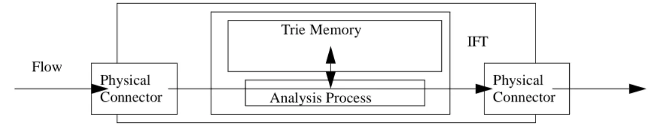
The performance of the cell-level analyzer is bounded by two parameters depicted in Figure 20. The first one is the physical connector linking the IFTs to the cell analysis automaton. The type of this physical con-nector is currently OC12. As a result, the maximum throughput supported by this concon-nector is 620Mb/s at the physical level. However, this physical throughput includes the overhead generated by the physical layer. Consequently the maximum throughput provided by the physical layer to the analysis process located in the ATM layer is 599Mb/s [28].
FIGURE 20. BASIC IFT INTERNAL DESCRIPTION.
The performance of the analysis process is also bounded by the capacity of the classification algorithm pre-sented in section 4. As demonstrated in section 4, the temporal complexity of our algorithm only depends on the number and sizes of the fields to be analyzed and on the size of the bit slice analyzed at each memory cycle. The current size of the bit slice is 4 bits. As depicted in Table 4, we currently need to analyze 9 fields. Table 4 describes the number of cycles needed to analyze each field, given the size of the field and the type of jump needed to move from one field to the next one in the analysis process. The type of jump is impor-tant, since non sequential jumps require more time than sequential ones. As a result, the maximal number of memory cycles needed to analyze a whole ATM cell is 51 memory cycles when the reordering scheme is not
IFT Physical Connector Physical Connector Analysis Process Trie Memory Flow
used, and 67 memory cycles when the reordering scheme is used. The difference between these two numbers is explained by the fact that jumps between fields are always supposed to be relatives when the reordering scheme is used.
TABLE 4. ANALYSIS PROCESS TIMING MODEL.
The value of a memory cycle is currently based on two FPGA (Field Programmable Gate Arrays) compo-nents and a single ZBT (Zero Bus Turnaround) memory chip allowing a bit slice to be analyzed in 15ns. However, we plan to use faster components in the future, allowing a 12ns memory cycle to be provided [29]. Table 5 provides the maximal analysis delay, the minimal classification speed (in million cells per second - Mc/s), and minimal classification throughput (in million bits per second - Mb/s) for each one of these mem-ory cycles when the minimal size to analyze equals an ATM cell (53 bytes). Note that this case can only hap-pen when no SNAP/LLC is used, since the minimal frame size with a SNAP/LLC encapsulation in any other case is 52 bytes.
TABLE 5. CLASSIFICATION CAPACITIES.
In the case of a 12ns memory cycle, without the reordering scheme, our classification algorithm cannot be considered as the blocking element of our access-control architecture since the minimal classification throughput is bigger than the maximal throughput that can be provided by the physical connector. As a result the maximal delay that can be introduced by our access-control architecture in this case is at most 612ns. In the case of a 15ns memory cycle or when the reordering technique is used, the previous property is no longer true since the throughput provided by the physical connector can be bigger than the throughput the analysis process is able to treat. As a consequence, it is interesting to examine in which conditions our anal-ysis process can be overwhelmed by classification requests. Table 5 describes the part of the traffic that has to be generated by an attacker in order to generate a denial of service attack on our classification scheme. This traffic is supposed to meet the most stringent conditions (One packet per cell requiring the analysis of 9
Field Size (bits) Type of jump Memory cycles (Wo. Reordering)
Memory cycles (W. Reordering)
Process start overhead 2 2
VCI 16 Relative 8 8
Encapsulation 4 Relative 5 5
Version 4 Sequential 1 5
Header Length 4 Relative 5 5
Source Addres 32 Sequential 8 12
Destination Address 32 Sequential 8 12
Source Port 16 Sequential 4 8
Destination Port 16 Relative 8 8
TCP Flags 8 / 2 2
TOTAL 51 67
Memory cycle Reorder
. Analysis delay Classification speed Min. Classification throughput Avg. Classification throughput DoS 12 ns No 612 ns 1.634 Mc/s 692.8 Mb/s 5224 Mb/s >100% Yes 804 ns 1.243 Mc/s 527.4 Mb/s 3977 Mb/s 98% 15 ns No 765 ns 1.307 Mc/s 554.6 Mb/s 4182 Mb/s 99% Yes 1005 ns 0.995 Mc/s 421.9 Mb/s 3184 Mb/s 94%