Algorithms for Passive Dynamical Modeling and
Passive Circuit Realizations
by
Zohaib Mahmood
B.Sc., University of Engineering and Technology, Lahore, Pakistan
(2007)
S.M., Massachusetts Institute of Technology (2010)
Submitted to the Department of Electrical Engineering and Computer
Science
in partial fulfillment of the requirements for the degree of
Doctor of Philosophy in Electrical Engineering and Computer Science
at the
MASSACHUSETTS INSTITUTE OF TECHNOLOGY
February 2015
c
⃝ Massachusetts Institute of Technology 2015. All rights reserved.
Author . . . .
Department of Electrical Engineering and Computer Science
January 08, 2015
Certified by . . . .
Luca Daniel
Emanuel E. Landsman Associate Professor of Electrical Engineering
Thesis Supervisor
Accepted by . . . .
Leslie A. Kolodziejski
Chairman, Department Committee on Graduate Theses
Algorithms for Passive Dynamical Modeling and Passive
Circuit Realizations
by
Zohaib Mahmood
Submitted to the Department of Electrical Engineering and Computer Science on January 08, 2015, in partial fulfillment of the
requirements for the degree of
Doctor of Philosophy in Electrical Engineering and Computer Science
Abstract
The design of modern electronic systems is based on extensive numerical simulations, aimed at predicting the overall system performance and compliance since early de-sign stages. Such simulations rely on accurate dynamical models. Linear passive components are described by their frequency response in the form of admittance, impedance or scattering parameters which are obtained by physical measurements or electromagnetic field simulations. Numerical dynamical models for these components are constructed by a fitting to frequency response samples. In order to guarantee sta-ble system level simulations, the dynamical models of the passive components need to preserve the passivity property (or inability to generate power), in addition to being causal and stable. A direct formulation results into a non-convex nonlinear optimization problem which is difficult to solve.
In this thesis, we propose multiple algorithms that fit linear passive multiport dynamical models to given frequency response samples. The algorithms are based on convex relaxations of the original non-convex problem. The proposed techniques improve accuracy and computational complexity compared to the existing approaches. Compared to sub-optimal schemes based on singular value or Hamiltonian eigenvalue perturbation, we are able to guarantee convergence to the optimal solution within the given relaxation. Compared to convex formulations based on direct Bounded-Real (or Positive-Real) Lemma constraints, we are able to reduce both memory and time requirements by orders of magnitude. We show how these models can be extended to include geometrical and design parameters.
We have applied our passive modeling algorithms and developed new strategies to realize passive multiport circuits to decouple multichannel radio frequency (RF) arrays, specifically for magnetic resonance imaging (MRI) applications. In a coupled parallel transmit array, because of the coupling, the power delivered to a channel is partially distributed to other channels and is dissipated in the circulators. This dissipated power causes a significant reduction in the power efficiency of the overall system. In this work, we propose an automated eigen-decomposition based approach to designing a passive decoupling matrix interfaced between the RF amplifiers and the
coils. The decoupling matrix, implemented via hybrid couplers and reactive elements, is optimized to ensure that all forward power is delivered to the load. The results show that our decoupling matrix achieves nearly ideal decoupling. The methods presented in this work scale to any arbitrary number of channels and can be readily applied to other coupled systems such as antenna arrays.
Thesis Supervisor: Luca Daniel
Acknowledgments
I would like to thank Professor Luca Daniel for his constant support and guidance
over the last several years. I am grateful to him for all the creative discussions we have had which inspired several new ideas presented in this research. It would not
have been possible for me to complete this research without his advice and constant mentoring.
I am grateful to Professor Jacob White and Professor Elfar Adalsteinsson for being on my PhD Committee. In addition to my thesis supervisor and committee
members I would like to thank my mentors including Professor Lawrence L Wald, Professor Roberto Suaya, Professor Stefano Grivet-Talica and Professor Giuseppe
Carlo Calafiore. I am obliged to all of them for their time and feedback on my research.
I am greatly indebted to Brad Bond for getting me started with this new field.
Our first interaction started when he was a Teaching Assistant for the course 6.336 Introduction to Numerical Simulation. I never missed his office hours. I am thankful
to Prof. Luca and Dr. Brad for making 6.336 such an exciting experience. Later we continued to collaborate very closely on different topics including nonlinear system
identification and some of the research presented in this thesis. I am grateful to him for always welcoming technical discussions. He has been a great source of learning
and inspiration for me.
Working with the Computational Prototyping Group has been a great pleasure.
I would like to thank all current and past members of our group for very useful discussions.
I would like to thank the MIT Office of the Provost for awarding me the Irwin
Mark Jacobs and Joan Klein Jacobs Presidential Fellowship, which supported my research during my first year at MIT. I am grateful to all the funding sources that
funded various projects during my PhD.
Last, but definitely not the least, I am wholeheartedly thankful to my family for
Contents
1 Introduction 13
1.1 Motivation . . . 13
1.2 Overview and Contributions of this Thesis . . . 15
1.3 Organization of this Thesis . . . 16
2 Background 17 2.0.1 Notations . . . 17
2.1 Linear Time Invariant (LTI) systems . . . 17
2.2 Passivity . . . 18
2.2.1 Manifestation of Passivity for a Simple RLC Network . . . 20
2.3 Tests for Certifying Passivity . . . 20
2.3.1 Tests Based on Solving a Feasibility Problem . . . 20
2.3.2 Tests Based on Hamiltonian Matrix . . . 21
2.3.3 Sampling Based Tests - Only Necessary . . . 22
2.4 Convex Optimization Problems . . . 22
2.4.1 Convex and Non-Convex Functions . . . 22
2.4.2 Convex Optimization Problems . . . 23
2.4.3 Semidefinite Programs . . . 24
3 Existing Techniques 25 3.1 Traditional Approaches . . . 25
3.2 Automated Approaches . . . 27
3.3.1 The Traditional Projection Framework . . . 27
3.3.2 Stable Projection for Linear Systems . . . 28
3.3.3 Parameterization of Projection Methods . . . 29
3.4 Rational Fitting of Transfer Functions . . . 30
3.4.1 One-step Procedures . . . 32
3.4.2 Two-steps Procedures . . . 32
3.4.3 Parameterized Rational Fitting . . . 34
4 Passive Fitting for Multiport Systems - Method I 37 4.1 Rational Transfer Matrix Fitting in Pole Residue Form . . . 38
4.2 Passive Fitting for Multiport LTI Systems . . . 39
4.2.1 Problem Formulation . . . 39
4.2.2 Conjugate Symmetry . . . 39
4.2.3 Stability . . . 40
4.2.4 Positivity . . . 41
4.2.5 The Constrained Minimization Problem . . . 43
4.3 Implementation . . . 44
4.3.1 Step 1: Identification of Stable Poles . . . 44
4.3.2 Step 2: Identification of Residue Matrices . . . 45
4.3.3 Equivalent Circuit Synthesis . . . 48
4.3.4 The Complete Algorithm . . . 49
4.4 Proposed Unconstrained Minimization Setup . . . 50
4.4.1 Notations . . . 50
4.4.2 Computing The Equivalent Function . . . 51
4.4.3 Computing The Jacobian Matrix . . . 53
4.5 Results . . . 55
4.5.1 Wilkinson Combiner in a LINC Amplifier . . . 55
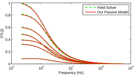
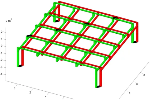
4.5.2 Power & Ground Distribution Grid . . . 58
4.5.3 On-Chip RF Inductors . . . 60
4.5.5 4-Port Structure . . . 63
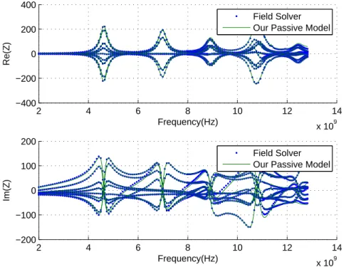
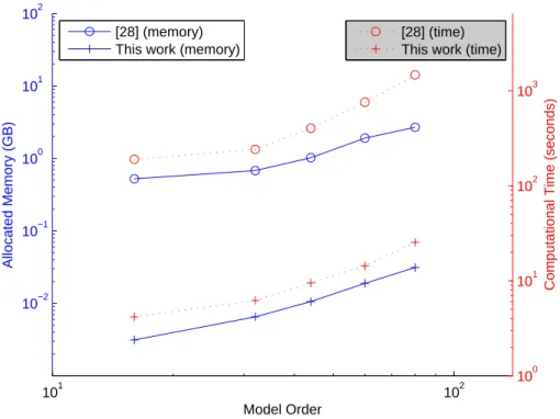
4.5.6 16-Port Structure . . . 65
4.5.7 60-Port Structure . . . 66
4.5.8 General Discussion . . . 68
5 Passive Fitting for Multiport Systems - Method II 71 5.1 Background . . . 72
5.1.1 Problem Description . . . 73
5.1.2 Computation of theH∞ Norm . . . 75
5.1.3 Localization Methods . . . 76
5.2 Passivity Enforcement using Localization Methods . . . 81
5.2.1 Initialization . . . 81
5.2.2 Passivity Enforcement Using The Ellipsoid Algorithm . . . 84
5.2.3 Passivity Enforcement Using The Cutting Plane Method . . . 86
5.2.4 Piecewise Linear Lower Bound on the Global Optimum . . . . 88
5.3 Results . . . 90
5.3.1 Example 1: A 4-Port PCB Interconnect Structure . . . 90
5.3.2 Example 2: A 4-Port Transformer . . . 92
5.3.3 Example 3: Handling Large Passivity Violations . . . 93
5.3.4 Example 4: Wide Bandwidth Passivity Violation . . . 97
5.3.5 Example 5: A packaging interconnect . . . 99
5.3.6 Example 6: A SAW Filter . . . 100
5.3.7 General Discussion . . . 102
6 Globally Passive Parameterized Model Identification 105 6.1 Motivation . . . 105
6.2 Background . . . 106
6.2.1 Interpolatory Transfer Matrix Parameterization . . . 106
6.2.2 Positivity of Functions . . . 108
6.3 Optimal Parameterized Fitting . . . 109
6.3.2 Rational Least Squares Fitting . . . 111
6.3.3 Linear Least Squares . . . 112
6.3.4 Polynomial Basis Example . . . 113
6.3.5 Complexity of Identification . . . 113
6.4 Constrained Fitting for Stability . . . 114
6.4.1 Stable Pole Fitting . . . 114
6.5 Constrained Fitting For Passivity . . . 116
6.5.1 Parameterized Residue Matrices . . . 116
6.5.2 Positive Definite Direct Matrix . . . 117
6.6 Implementation . . . 117
6.6.1 Individual Model Identification and Preprocessing . . . 117
6.6.2 Parameterized Identification Procedure . . . 118
6.6.3 Post-processing Realization . . . 119
6.7 Results . . . 120
6.7.1 Single port - Single parameter: Microstrip Patch Antenna . . 120
6.7.2 Multi port - Single parameter: Wilkinson Power Divider . . . 122
6.7.3 Multi port - Multi parameter: T-Type Attenuator . . . 125
7 Design of Decoupling Matrices for Parallel Transmission Arrays 131 7.1 Introduction . . . 131
7.2 Background . . . 134
7.2.1 Decoupling Conditions . . . 134
7.2.2 Interconnection of Circuit Blocks . . . 135
7.3 Design of a Decoupling Matrix . . . 136
7.3.1 The Four Stages of decoupling . . . 137
7.3.2 A Full Rank Transformation . . . 139
7.3.3 Realization of the SA/B . . . 139
7.3.4 Robustness Analysis . . . 141
7.3.5 Required Components . . . 142
7.4 Results . . . 143
7.4.1 A 2-channel example with hardware implementation . . . 143
7.4.2 A 4-channel example (simulations only) . . . 146
7.5 Discussion . . . 146
8 Conclusion 149 A Semidefintie Programming 151 A.1 Minimizing Quadratic Function . . . 151
A.2 Implementing Linear Matrix Inequalities . . . 153
B Definitions 155 B.0.1 Gradients and Subgradients . . . 155
B.0.2 Hyperplanes . . . 156
B.0.3 Ellipsoids . . . 156
B.0.4 Polyhedra . . . 157
C Derivations 159 C.1 Derivation of the weighted objective function . . . 159
C.2 Derivation of (5.16) . . . 159
Chapter 1
Introduction
1.1
Motivation
Generation of accurate and passive dynamical models for linear multiport analog
circuit blocks is a crucial part of the design and optimization process for complex integrated circuit systems. Quite often, these models also need to capture
depen-dence of the system on design and geometrical parameters while providing apriori passivity and stability certificates for the entire parameter range of interest. These
identified models are interfaced with commercial circuit simulators where they are
used to perform transient simulations being interconnected with other circuit blocks. In order to guarantee robust and stable numerical simulations, these models must sat-isfy physical properties such as causality, stability and passivity [119, 126]. Causality
and stability can be easily enforced during the model fitting [33, 34, 59, 63]. Passivity
enforcement is instead more challenging and requires special care. In this thesis we focus on generating guaranteed passive linear dynamical models.
Let us consider the typical design flow for an analog circuit block, say a distributed
power amplifier, containing on-chip multiport passive interconnect structures, such as multi-primary transformers for power combining. The full system design is
com-pleted in two steps. As the first step, the interconnect passive structures are laid out in an electromagnetic field solver and then simulated for frequency response in
based on the frequency samples or system matrices extracted by the solver which can
be incorporated into a circuit simulator (e.g. Spice or Spectre).
Equivalent Multiport Model
Figure 1-1: The model of a multiprimary transformer interfaced with circuit simulator to perform full distributed power amplifier simulations
Once the models are generated, they are interfaced with the circuit simulators
using either equivalent netlists or behavioral descriptions. The final network in Figure 1-1 shows the interconnection of the generated model with other building blocks of
the amplifier such as transistors and capacitors. Transient simulations are performed in order to get performance metrics of the complete nonlinear power amplifier. If the
generated model encounters a violation of any basic physical property of the structure,
such as passivity, it can cause huge errors in the response of the overall system, and the results may become completely nonphysical.
In addition, the designers would greatly benefit from these models if they are parameterized in some of the design parameters, such as width and spacing for an
inductor or characteristic impedance in the case of distributed transmission line struc-tures. These parameterized models will greatly reduce the design cycle by allowing the
designer to instantiate the structure with various design parameters without perform-ing another full-wave electromagnetic simulation. However these models are useful
only if the final parameterized models come with apriori passivity certificates in the entire parameter range of interest.
These models can also be used to realize passive networks. Although this is a well studied problem for single and two port networks. The problem of synthesizing a
devices. In this thesis we propose strategies to automatically design realizable
net-works from the given response. We have explored applications including the design and practical realization of decoupling matrices (or multiport matching networks) to
decouple Radio Frequency (RF) phased arrays for Magnetic Resonant Imaging (MRI) applications.
1.2
Overview and Contributions of this Thesis
In this thesis we propose various algorithms to automatically generate both individual
non-parameterized and parameterized passive multiport models, and passive circuit realizations. In particular the main contributions of this thesis are summarized as
follows:
• We have proposed an algorithm to identify individual passive dynamical models. The proposed algorithm identifies the unknown system in two steps. The first
step is to identify a common set of stable poles for the multiport structure. The second step is to identify residue matrices which conform to passivity conditions.
These passivity conditions are enforced as Linear Matrix Inequalities (LMIs) [82,
90].
• We have proposed another passive model identification algorithm which is based on a parameterization of general state-space scattering models with fixed poles.
We formulate the passivity constraints as a unitary boundedness condition on theH∞norm of the system transfer function. We solve the resulting convex non-smooth optimization problem via computationally efficient localization based algorithms, such as the ellipsoid and the cutting plane methods [85, 86, 89].
• We have proposed a new strategy to develop globally stable and passive pa-rameterized models. In this approach a collection of individual passive models is approximated by a single closed form model which conforms to passivity
• We have extended our passive modeling algorithms and proposed automated strategies to design a robust decoupling matrix (or multiport matching net-work) interfaced between the RF amplifiers and the coils in a multi channel
transmission array. Our decoupling matrix mixes the input signals and is opti-mized to ensure all forward power is delivered to the load [83, 84].
The matlab implementations of various algorithms proposed in this thesis is posted on public domain as free open source software at http://www.rle.mit.edu/cpg/ and [1].
1.3
Organization of this Thesis
This thesis is organized as follows: Chapter 2 covers the relevant background on
linear systems and passivity. Chapter 3 describes a brief overview of the existing techniques along with their advantages and shortcomings. Chapter 4 explains our
convex formulation identifying passive system models in pole residue form. Chapter 5 presents our algorithm identifying passive linear system models using localization
methods. Chapter 6 presents details on how the proposed algorithm can be extended to identify globally passive parameterized models with apriori passivity certificates.
Chapter 7 describes how our passive modeling algorithms can be extended to design decoupling matrices for coupled arrays. Chapter 8 summarizes the thesis. Appendix A
describes how some of the convex problems can be cast as semidefinte programs. All the theoretical developments are supported by examples which are provided at the
Chapter 2
Background
2.0.1
Notations
We shall use the following notations in this section.
np = Number of ports of the given system (2.1)
κ = Number of poles (2.2)
q = Number of states of the compact model (2.3)
F = Number of frequency points (2.4)
2.1
Linear Time Invariant (LTI) systems
Dynamical systems are an extremely useful tool for the time-domain analysis of
physi-cal systems, as they provide a relationship between an input signal u(t) and an output signal y(t) for the system. In state-space models, the evolution of the system is
de-scribed by a state vector x(t), which is controlled by input u(t) and from which output y(t) is determined. In the general form, a Linear Time Invariant (LTI) state-space model can be expressed as
d(x)
dt = Ax(t) + Bu(t) (2.5)
y(t) = Cx(t) + Du(t)
where A ∈ Rq×q, B ∈ Rq×np, C ∈ Rnp×q, and D ∈ Rnp×np. Here q and n p are the number of states and ports respectively. Linear systems can also be expressed in
terms of a transfer matrix, by applying Laplace transform of (2.5), as
H(s) = Y (s) U (s) , C(sI − A) −1B + D = H11(s) · · · H1p(s) .. . . .. ... Hp1(s) · · · Hpp(s) (2.6)
Here Hij(s) indicates the transfer function from P ort j to P ort i.
2.2
Passivity
Passivity is one of the most important properties of dynamical systems. Passivity,
which is often referred to as dissipativity in other scientific communities, intuitively refers to the inability of a dynamical system to generate energy in addition to the
one already provided by external connections. As discussed in [119], passive models not only are physically consistent, but also guarantee numerically stable system-level
simulations. Non-passive models may instead lead to instability even when their terminations or loads are passive [51].
Consider a system described by input ( say current) u and output (say voltage)
y. Then ⟨u, y⟩τ describes the total energy of the system up to time τ , where
⟨u, y⟩τ = ∫ τ
−∞
Then the system is passive if
⟨u, y⟩τ ≥ 0, ∀τ ∈ R+ (2.8)
Linear systems are usually described as a transfer matrix or as a state space model. Let us consider the passivity of impedance or admittance systems specified by
a transfer matrix H(s). Passivity for an impedance or admittance system corresponds to ‘positive realness’ of the transfer matrix. To be positive real, the transfer matrix
ˆ
H(s) must satisfy the following constraints
H(¯s) = H(s) (2.9a)
H(s) is analytic in ℜ s > 0 (2.9b)
H(jω) + H(jω)†≽ 0 ∀ω (2.9c)
Where ℜ denotes the real part and † indicates the conjugate transpose.
The first condition (2.9a), commonly known as conjugate symmetry, ensures that
the impulse response corresponding to H(s) is real. The second condition (2.9b) implies stability of the transfer function. A causal linear system in the transfer
matrix form is stable if all of its poles are in the left half of the complex plane, i.e. all the poles have negative real part. The system is marginally stable if it has simple
poles (i.e. poles with multiplicity one) on the imaginary axis. The third and final condition (2.9c), which is the positivity condition, implies positive realness of the
2.2.1
Manifestation of Passivity for a Simple RLC Network
We consider a simple RLC network as shown in Figure 2-1. In this simple schematic we can analytically compute the equivalent of passivity conditions as follows
Zeq(ω) = R + jXeq(ω)
= R + j ωL
1− ω2LC (2.10)
Here ℜZeq = R. The passivity condition translates into R being non-negative, i.e. R≥ 0 in addition to L and C being non-negative.
Figure 2-1: Manifestation of passivity for a simple RLC network where Zeq(ω) = R + jXeq(ω). Passivity implies that R, L, C ≥ 0
2.3
Tests for Certifying Passivity
There are several tests, all based on positive real lemma, by which a model can be
certified to be passive. Section 2.3.1 and 2.3.2 describe conditions which are both necessary and sufficient for passivity [16]. Section 2.3.3 describes a necessary condition
for passivity.
2.3.1
Tests Based on Solving a Feasibility Problem
Ed(x)
dt = Ax + Bu
y = Cx + Du
with minimal realization (i.e. every eigenvalue of A is a pole of H(s)), passivity is implied by the positive real lemma. The positive real lemma states that if there
exists a positive definite matrix P = PT ≻ 0 and P ∈ Rq×q such that the following matrix is negative semidefinite
ETP A + ATP E ETP B− CT BTP E− C −D − DT
≼ 0 (2.11)
then H(s) is positive real and hence the system is passive. In order to certify if a system is passive, the feasibility problem for the existence of a positive definite matrix
P = PT ≻ 0 can be solved. However such a formulation will result into a non-linear non-convex problem which may not be solved efficiently.
2.3.2
Tests Based on Hamiltonian Matrix
We can solve a condition equivalent to (2.11) based on Riccati equations and Hamil-tonian Matrices. If we assume that D + DT ≻ 0, then the inequality (2.11) is feasible if and only if there exists a real matrix P = PT ≻ 0 satisfying the Algebraic Riccati Equation
ATP + P A + (P B− CT)(D + DT)−1(P B− CT)T = 0 (2.12)
Hamiltonian matrix M as follows A− B(D + DT)−1C B(D + DT)−1BT −CT(D + DT)−1C −AT + CT(D + DT)−1BT . (2.13)
Then the system (2.5) is passive, or equivalently, the LMI (2.11) is feasible, if and only if M has no pure imaginary eigenvalues [16].
2.3.3
Sampling Based Tests - Only Necessary
Another class of passivity tests are based on checking the passivity conditions (2.9) at discrete frequency samples. Since passivity requires condition (2.9) to hold for all
ω, a reduced model is non-passive if λmin(ℜ{H(jωi)}) < 0 only for some ωi. Here
λ denotes the eigen values. Note that this test is based on a necessary condition and can only be used to check data samples or samples from the model for passivity violations and cannot be used to certify the passivity of a model.
2.4
Convex Optimization Problems
In this section we describe general convex optimization problems. Before discussing the optimization problems, we first describe the notion of convexity and convex
func-tions in the following section. For detailed description we refer the readers to [19].
2.4.1
Convex and Non-Convex Functions
A function f (x) is convex if the domain of f (x) is convex and if for all x, y ∈ domain f (x) and θ∈ [0, 1], it satisfies
f (θx + (1− θ)y) ≤ θf(x) + (1 − θ)f(y) (2.14)
Geometrically, this inequality means that the line segment between (x, f (x)) and
Convex function
(finding global minimum is easy)
(x,f(x))
(y,f(y))
Figure 2-2: Shows a convex function. In general finding global minimum for convex functions is easy
One of the nice properties of a convex function is that they have only global minimum which is relatively easier to compute compared to non-convex functions, as
shown in Figure 2-3, which may have local minima and hence making the computation of global minimum an extremely difficult task.
Non-convex function
(finding global minimum is extremely difficult)
Figure 2-3: Shows a convex function. In general finding global minimum for convex functions is extremely difficult
2.4.2
Convex Optimization Problems
minimize f0(x)
subject to fi(x)≤ 0, i = 1, . . . , m aTi x = bi, i = 1, . . . , p
(2.15)
where the objective function f0(x) is convex, the inequality constraint functions
fi(x) are convex and the equality constraint functions hi(x) = aTi x− bi are affine. Hence in a convex optimization problem we minimize a convex objective or cost function over a convex set. Convex optimization problems are particularly attractive
since finding global minimum for the cost function is a relatively easy.
2.4.3
Semidefinite Programs
Semidefinte Programs or simply SDPs belong to a special type of convex optimization
problems where a linear cost function is minimized subject to linear matrix inequali-ties.
minimize cTx
subject to F1x1+ F2x2+· · · + Fnxn− F0 ≽ 0
(2.16)
where all of the matrices F0, F1, . . . Fn ∈ Sk, here Sk indicates set of symmetric matrices of order k× k. Semidefinite Programs are particularly important since most of the convex optimization problems can be cast as an SDP (described in Appendix A) and can be solved efficiently using public domain solvers such as [2, 100].
Chapter 3
Existing Techniques
System level analysis of modern electronic systems are based on extensive numerical
simulations, aimed at predicting the overall system performance and compliance since early design stages. Such simulations rely on accurate component dynamical models
that prove efficient when used in standard circuit simulators. Over the last few years many techniques [15,22,23,28,31,33,34,36,46,48,50,52,53,57,59–64,68,74,79,80,86,87,
90,102–104,107,108,112,119,120,126] have been developed for the generation of linear dynamical models. In this chapter we summarize various existing techniques for
non-parameterized and non-parameterized model generation of multiport passive structures.
3.1
Traditional Approaches
Traditionally, the critical task of generating a model is completed manually that is the circuit designer or system architect approximates the unknown system with
emprirical or semi empirical formulas. These models rely on the designers’ experience and intuition accumulated after a lifetime of simulations with electromagnetic field
solvers and circuit simulators. In these approaches, normally the designer would either approximate the structure with lumped RC and RL networks characterized at
the operating frequency as shown in Figure 3-1 or generate a simple schematic from intuition consisting of RLC elements having frequency response ‘close’ to the original
Figure 3-1: Approximation at operating frequency
Figure 3-2: Approximation from intuition or basic physics
Unfortunately, these intuitive approaches have limited applications and may not
capture all the important features in a given frequency response. Additionally, in order to generate a complete multiport transfer matrix, quite often these approaches
approximate the individual transfer functions separately. Hence, these models may be completely nonphysical, violating important physical properties of the original
system such as passivity, since passivity is a property of the entire transfer matrix and cannot be enforced if transfer functions are identified individually. Also, these
techniques are not scalable, hence generating a model for a system with more than a few ports may become challenging. Furthermore, the modeling task becomes even
more difficult when attempting to generate by hand closed form compact models of the frequency response parameterized by design or geometrical parameters.
In order to make this process more efficient and robust, it is desirable to replace
hand-generated macromodels by automatically-generated compact dynamical mod-els that come with guarantees of accuracy, and passivity. In the following sections
dynamical models.
3.2
Automated Approaches
In the recent years, considerable effort has been put into automating the procedure to generate compact parameterized models. There are two commonly used techniques to
generate models for linear structures. The first ones are projection based approaches and the second ones are rational fitting approaches. A detailed survey of these
ap-proaches is presented in [14]. We describe these techniques one by one in the following sections.
3.3
Projection Based Approaches
3.3.1
The Traditional Projection Framework
Most of the model order reduction techniques can be interpreted within a projection framework. In such a framework the solution to a given large linear multiport system
E ˙x = Ax + Bu, y = CTx, (3.1)
is approximated in a low-dimensional space x ≈ V ˆx, where V ∈ Rq×qr is the right projection matrix, ˆx is the reduced state vector, and q >> qr. A reduced set of equations is then obtained by forcing the residual, r(V ˆx) = EV ˙ˆx− AV ˆx − Bu, to be orthogonal to the subspace defined by a left projection matrix U , i.e. UTr(V ˆx) = 0. The resulting state space model has the form
ˆ
E ˙ˆx = ˆAˆx + ˆBu, y = ˆCTx,ˆ (3.2)
the reduced model created via projection is completely determined by the choice
of projection matrices U and V . The most common approaches for selecting the vectors are methods based on balanced truncation, moment matching, and singular
value decomposition (e.g. proper orthogonal decomposition, principle components analysis, or Karhunen-Loeve expansion). For more details on generating projection
vectors see [11, 56].
3.3.2
Stable Projection for Linear Systems
Traditionally it is assumed that the original large system (3.1) possesses an extremely special structure viz. E = ET ≽ 0, A ≼ 0, and B = C. In such cases selecting U = V (known as congruence transform or Galerkin projection) will preserve stability and passivity in the reduced system for any choice of V . While all digital RLC type
inter-connect networks possess the required semidefinite structure, for analog modeling it is, unfortunately, completely unrealistic to restrict consideration to only semidefinite
systems. Therefore for the vast majority of analog systems, the congruence trans-form cannot guarantee stability and passivity of the generated model. One possible
computationally cheap solution is to use as a first step any of the available tradi-tional projection based methods (including congruence transforms) and then attempt
to perturb the generated model to enforce stability and passivity. One semidefinite formulation of this problem is
minimize ∆ ˆE,∆ ˆA,∆ ˆC ||∆ ˆ E|| + ||∆ ˆA|| + ||∆ ˆC|| subject to Eˆ ≽ 0, ˆ A + ˆAT ≼ 0, ˆ B = ˆC (3.3)
where ˆE = UTEV + ∆ ˆE, ˆA = UTAV + ∆ ˆA, ˆB = UTB, and ˆC = VTC + ∆ ˆC. Here
stability and passivity are enforced in the reduced model by forcing it to be described by semidefinite system matrices, which introduced no loss of generality even if the
Unfortunately, in most cases any such perturbation could completely destroy the
accuracy of the reduced model. Instead of perturbing the reduced model , a better approach that can guarantee accuracy in the reduced model is to perturb one of the
projection matrices. That is, given U and V , search for a ‘small’ ∆U such that the system (3.2), defined by reduced matrices ˆE = (U +∆U )TEV, ˆA = (U +∆U )TAV, ˆB =
(U +∆U )TB, and ˆC = VTC+∆ ˆC is passive. This problem can similarly be formulated as a semidefinite program minimize ∆U ||∆U|| subject to Eˆ ≽ 0, ˆ A + ˆAT ≼ 0, ˆ B = ˆC (3.4)
It can be shown that if the original model (3.1) is stable and passive, then for any projection matrix V there exist projection matrices U such that the resulting reduced
model is stable and passive [13].
3.3.3
Parameterization of Projection Methods
Generating a parameterized reduced model, such as
ˆ
E(λ) ˙ˆx = ˆA(λ)ˆx + ˆB(λ)u (3.5)
for a linear system where λ is a vector of design parameters, is of critical impor-tance if the models are to be used for system level design trade-off explorations. Two
modifications to the previously described projection procedures must be made when constructing parameterized models. First the subspace defined by V must capture
the solution response to changes in parameter values. Expanding the subspace is typically achieved for linear systems by generating projection vectors that match the
frequency [29, 125]. Alternative approaches for handling variability resulting from a
large number of parameters are based on sampling and statistical analysis [38, 133].
The second issue involves specifically the case of nonlinear parameter dependence, where the system matrix or vector field must be able to cheaply capture changes in
λ. One way to make a parameterized system matrix A(λ) projectable with respect to the parameters is to represent them as a sum on non-parameterized functions
that are linear in scalar functions of the original parameters. For instance, for the parameterized linear system
˙x = A(λ)x (3.6)
we seek to approximate and project as follows:
A(λ)≈ κ ∑ i=0 ˜ Aigi(λ)→ ˆA(λ)≈ κ ∑ i=0 (UTAiV )gi(λ) (3.7)
such that ˆAi = UTAiV are constant matrices and can be precomputed. Here
gi(λ) are scalar functions of the original parameter set λ. The matrix approximation in (3.7) can be achieved using a polynomial expansion if A(p) is known analytically,
or via fitting in the case when only samples of the matrix Ak = A(λk) are known [29].
3.4
Rational Fitting of Transfer Functions
Projection methods have been successful for certain classes of linear systems, but in
many applications, such as when modeling analog passive components affected by full-wave effects or substrate effects, the resulting system matrices include delays, or
frequency dependency. To capture such effects in a finite-order state-space model, one must approximate this frequency dependence, using for instance polynomial
challenging. Furthermore, often times only transfer function samples are available,
obtained possibly from measurements of a fabricated device or from a commercial electromagnetic field solver. In such a scenario, since original matrices are not
avail-able, projection based approaches cannot be used.
An alternative class of methods are based on transfer matrix fitting. There exist
different approaches to generate rational transfer function matrices from frequency response data [34, 59, 68, 79, 107]. The problem of finding a passive multiport model
from complex frequency response data is highly nonlinear and non convex. Given a set of frequency response samples {Hi, ωi}, where Hi = H(jωi) are the transfer matrix samples of some unknown multiport linear system, the compact modeling task is to construct a low-order rational transfer matrix ˆH(s) such that ˆH(jωi)≈ Hi. Formulated as an L2 minimization problem of the sum of squared errors, it can be written as minimize ˆ H ∑ i Hi− ˆH(jωi) 2 subject to H(jω)ˆ passive (3.8)
Even after ignoring the passivity constraint in (3.8), the unconstrained minimiza-tion problem is non-convex and is therefore very difficult to solve. Direct soluminimiza-tion
using nonlinear least squares have been proposed, such as Levenberg-Marquardt [93]. However, there is no guarantee that such approach will converge to the global
mini-mum, and quite often the algorithm will yield only a locally optimal result. Rather than solving non-convex minimization problem, many methods apply a relaxation to
the objective function in (3.8) resulting in an optimization problem that can be solved efficiently. These methods differ in the way the cost function and the passivity
con-straints are formulated, and in the way the resulting optimization problem is solved. All of these approaches represent different points in a trade-off between
computa-tional cost and optimality of the solution. We consider a solution as optimal when it represents the most accurate passive model in the considered parameterization class,
clas-sified into one-step and two-steps procedures. One-step procedures simultaneously
enforce passivity during the fitting process by using a convex or quasi-convex re-laxation [80, 112]. Two-steps procedures first generate a stable (but not necessarily
passive) model. Passivity is enforced during the second step [23, 28, 31, 36, 87, 90].
3.4.1
One-step Procedures
Over the past years considerable effort has been put into finding a convex relaxation to the original problem including the passivity constraint (3.8) such as [80, 112].
These techniques lie on the more optimal but less efficient side of the trade-off. The technique in [112] (available for download at [4]) presents a quasi-convex relaxation,
with the advantage of simultaneous optimization of both model poles and residues including passivity constraints. This approach has also been extended in [112] to
the generation of parameterized passive models. Although optimal, this formulations may require possibly large computational costs both in terms of memory and CPU
time for systems with a large number of parameters.
3.4.2
Two-steps Procedures
A suboptimal but potentially more efficient class of methods uses a ‘two-steps’ pro-cedure. In the first step, poles and residues are fitted extremely efficiently without
considering passivity constraints [59]. In a second step the poles are kept fixed and the residues are then optimized based on a variety of cost functions, passivity constraints
and optimization techniques.
Passivity via Perturbation
Many of the ‘two-steps’ methods employ a perturbation framework in the second step [15, 46, 50, 52, 57, 64, 102, 103, 108], where passivity violations are corrected iteratively.
These techniques are computationally very efficient. However their main drawback is that the underlying formulation does not guarantee convergence of the algorithm
non-optimal in terms of accuracy. Some of these methods are based on iterative
perturbation of the frequency dependent energy gain of the model ( [60, 62, 102, 103]) through the solution of approximated local problems. Variants of the above schemes
have been presented in [53, 61, 74, 104, 120]. A comprehensive comparison of such passive linear dynamical modeling techniques is available in [48]. In the following
sections, we describe two approaches relevant to this thesis.
Passivity Enforcement Using Linear Matrix Inequalities
Within these ‘two-steps’ methods, some approaches guarantee optimality in the sec-ond step exploiting convex or quasi-convex formulations ( [23, 28, 31, 36, 87, 90]). Such
algorithms enforce passivity by defining constraints based on the positive real lemma or the bounded real lemma [18, 98].
For example, passivity of a linear dynamical system described by scattering
rep-resentation can be directly enforced by the bounded real lemma (or by the positive real lemma for hybrid representation) [28]. Passivity enforcement via bounded real
lemma can be directly formulated as a semidefinite program (SDP) and solved using standard SDP solvers such as [117] to compute the global optimal solution.
minimize B,C,D,W ∑ i Hi − ˆH(jωi) 2 (3.9) subject to ATW + W A W B CT BTW −I DT C D −I ≼ 0 (3.10) W = WT ≽ 0
Problem (3.10) generates a passive model with optimal accuracy with in the class of
two-steps based methods (in these methods the poles and residues are calculated in two steps). The main drawback of these methods, however, is the excessive
This limits the scalability of SDP based passive model generation algorithms. Hence
the application of such algorithms is restricted to relatively smaller examples.
Passivity via Passive-Subsections
A model is passive if all of its building blocks are passive. There are approaches, such as [92,94], where the individual building blocks of a non-passive model are checked for
passivity individually. However, since such a condition is only a sufficient condition, many passive models will fail the test. Also in these approaches [92, 94] no efficient
method or algorithm was presented in order to rectify for passivity violations. For example in [94] it was proposed that the pole-residue pairs violating passivity
condi-tions should be discarded, this is highly restrictive and can significantly deteriorate the accuracy. We instead propose that the identified residue matrices should
con-form to passivity conditions during the identification such that there are no passivity violation in the final model.
3.4.3
Parameterized Rational Fitting
There are two possible approaches to generating a parameterized transfer matrix ˆ
H(s, λ) from a given set of frequency response and parameter values {Hi, ωi, λi}. The first approach is to fit simultaneously to the frequency response data and param-eter values, i.e. minimizing ∑| ˆH(jωi, λi)− Hi|2. This approach was first proposed in [112] along with the simultaneously enforcement of stability passivity. However, simultaneous frequency and parameter fitting can become quite expensive for a large
number of parameters. Alternative fitting approaches rely on interpolating between a collection of non-parameterized models, each generated by a stable and passive
fit-ting procedure. The main challenge for such approaches based on interpolation is to guarantee passivity in the final interpolated model, since one may produce very trivial
stable systems where simple interpolation will not preserve stability or passivity. All the current existing interpolation based algorithms [32, 40, 118] only provide a test to
instantiated. The downside of such methods is that the user (i.e. a circuit designer,
or a system level optimization routine) would need to run such test every single time a new model is instantiated. Furthermore, if the instantiated model does not pass the
stability test, the user would either be stuck with an unstable model, or would need to basically rerun the fitting algorithm to perturb the unstable instantiation until
sta-bility is achieved. In other words none of the available interpolation based approaches can guarantee that any instantiation of their identified parameterized models will be
a priori stable and passive for any value of the parameters in a predefined range. In this thesis we present a method for generating parameterized models of lin-ear systems that the user will be able to instantiate for any parameter value either within a limited given range, or for an unlimited range, and be sure a priori to obtain
a passive model. Given a collection of systems swept over design and geometrical
parameters of interest, we identify a closed form parameterized dynamical model using constrained fitting. The details can be found in Chapter 6. Our algorithm
is completely independent from the type of initial non-parameterized identification procedure used for the individual systems, if only stability is sought in the final
pa-rameterized model. In other words, the individual (non-papa-rameterized) models may be generated by any stability preserving modeling scheme such as convex
optimiza-tion based approaches [28, 81, 112], vector fitting based approaches [47, 49, 58, 59] or Loewner matrix based approaches [77]. However, in order to enforce global
passiv-ity, the individual non-parameterized models need to have the structure described in Chapter 4.
Chapter 4
Passive Fitting for Multiport Systems
- Method I
In this chapter we present a framework for identifying passive dynamical models from frequency response data. We cast the problem as a standard semidefinte program
(SDP) which can be solved by SDP solvers such as [2,100].We solve the problem in two steps. First a set of common poles is identified using already established techniques [5,
59, 112]. Next, we identify residue matrices while simultaneously enforcing passivity.
Theoretically our identified models are restrictive in the sense that we are enforcing passivity through a sufficient but not necessary condition, however in practice these
models can model most practical systems as is demonstrated in Section 4.5. By paying a small price in terms of accuracy we manage to solve larger problems within limited
computational resources, such as memory, and gain orders of magnitude improvement in terms of speed compared to [28, 112]. We remark that although [28, 112] can
generate more accurate models, their usability is limited to very small examples.
We use a framework similar to the one proposed in [82], however we overcome
the underlying challenges which arise from the decoupling of the two steps (i.e. iden-tification of stable poles and passive residues) by proposing an adaptive or assisted
pole placement algorithm which improves the stable pole placement. We have tested the algorithm on a set of challenging examples for which existing approaches do not
Note that sufficient only passivity conditions used in this chapter were also
de-rived in [92, 94]. However in [92, 94] these conditions were used only to ‘check’ for passivity violations. In our proposed algorithm, these conditions are instead built
into the model generation procedure to ‘enforce’ passivity. Also, no efficient algo-rithm was proposed in [92, 94] to rectify for passivity violations. For example in [94]
it was proposed that the pole-residue pairs violating passivity conditions should be discarded, this is highly restrictive and can significantly deteriorate the accuracy. We
instead propose that the identified residue matrices should conform to passivity
con-ditions during the model generation, such that there are no passivity violation in the final model. The formulation presented in this chapter, being convex, is guaranteed to converge to the global minimum and can be easily implemented using publicly
available convex optimization solvers such as SeDuMi [2].
4.1
Rational Transfer Matrix Fitting in Pole Residue
Form
The problem of constructing a rational approximation of multi port systems in pole
residue form consists of finding residue matrices Rk, poles akand the matrices D & F such that the identified model, defined by the transfer function ˆH(s) in (4.1),
mini-mizes the mismatch with the frequency response samples from the original system as described in (3.8). ˆ H(s) = κ ∑ k=1 Rk s− ak + D + sF (4.1)
here Rk, D and F are np×np residue matrices (assuming the system has np ports) and ak are poles. Since most of the passive structures have a symmetric response, we
consider the case when Rk, D and F are symmetric matrices. In the case when the
matrices are non-symmetric, we can apply the same formulation to the symmetric
4.2
Passive Fitting for Multiport LTI Systems
4.2.1
Problem Formulation
To formulate the problem, we expand the summation for ˆH(s) in (4.1) in terms of the
purely real and complex poles. Also, since we are mainly interested in the properties of H(s) on the imaginary axis, we replace s with jω.
ˆ H(jω) = κr ∑ k=1 Rr k jω− ar k + κc ∑ k=1 Rc k jω− ac k + D + jωF (4.2)
Where κr and κc denote the number of purely real and the number of complex
poles, respectively. Also, Rrk ∈ Rnp×np, Rc
k ∈ Cnp×np, ark ∈ R, ack ∈ C ∀k, and
D, F∈ Rnp×np.
In the following sections, we consider one by one the implications of each passivity condition in (2.9) on the structure of (4.2).
4.2.2
Conjugate Symmetry
Let us consider the implications of first condition of passivity on the structure of our proposed model in (4.2). The terms in (4.2) corresponding to the matrices D and
F, and to the summation over purely real poles satisfy automatically the property of
conjugate symmetry in (2.9a). On the other hand such condition requires that the
complex-poles ac
kand complex residue matrices Rckalways come in
complex-conjugate-pairs ˆ H(jω) = κr ∑ k=1 Rr k jω− ar k + κc/2 ∑ k=1 { ℜRc k+ jℑRck jω− ℜac k− jℑa c k + ℜR c k− jℑRck jω− ℜac k+ jℑa c k } + D + jωF (4.3)
In (4.3) ℜ and ℑ indicate the real and imaginary parts respectively. Note that the summation for complex poles now extends only upto κc/2.
Lemma 1 (Conjugate Symmetry) Let ˆH(jω) be a stable and conjugate symmetric
transfer matrix given by (4.3), then ˆH(jω) satisfy the property of conjugate symmetry ˆ
H(jω) = ˆH(jω).
Proof We show that the ˆH(jω), as in (4.3) satisfies ˆH(jω) = ˆH(jω) by construction.
ˆ H(jω) = κr ∑ k=1 Rr k −jω − ar k + κc/2 ∑ k=1 { ℜRc k+ jℑRck −jω − ℜac k− jℑack + ℜR c k− jℑRck −jω − ℜac k+ jℑack } + D− jωF ⇒ ˆH(jω) = κr ∑ k=1 Rr k jω− ar k + κc/2 ∑ k=1 { ℜRc k− jℑRck jω− ℜac k+ jℑack + ℜR c k+ jℑRck jω− ℜac k− jℑack } + D + jωF = ˆH(jω)
Rewriting (4.3) compactly we get:
ˆ H(jω) = κr ∑ k=1 ˆ Hkr(jω) + κc/2 ∑ k=1 ˆ Hkc(jω) + D + jωF (4.4) where: ˆHkr(jω) = R r k jω− ar k (4.5) ˆ Hkc(jω) = ℜR c k+ jℑRck jω− ℜac k− jℑack + ℜR c k− jℑRck jω− ℜac k+ jℑack (4.6)
4.2.3
Stability
The second condition (2.9b), which requires analyticity of ˆH(s) in ℜ{s} > 0, implies stability. For a linear causal system in pole-residue form (4.1), the system is strictly
stable if all of its poles ak are in the left half of complex plane i.e. they have negative real part (ℜ{ak} < 0). Note that the system is marginally stable if conjugate pair poles with multiplicity one are present on the imaginary axis.
4.2.4
Positivity
The positivity condition for passivity (2.9c) is the most difficult condition to enforce
analytically. We present here an extremely efficient condition which implies (2.9c). We consider the case when all the building blocks in the summation (4.4), namely:
purely real poles/residues ˆHkr(jω), complex-conjugate pairs of poles/residues ˆHkc(jω), and the direct term matrix D are individually positive real. Please note that the jωF
term has purely imaginary response and therefore does not affect positivity condition.
Lemma 2 (Positive Real Summation Lemma) Let ˆH(jω) be a stable and
conju-gate symmetric transfer matrix given by (4.4), then ˆH(jω) is positive-real if ˆHkr(jω), ˆ
Hc
k(jω) and D are positive-real ∀k. i.e.
ℜ ˆHkr(jω)≽ 0, ℜ ˆHkc(jω)≽ 0∀k & D ≽ 0 =⇒ ˆH(jω)≽ 0 (4.7) Proof The sum of positive-real, complex matrices is positive real.
Lemma 2 describes a sufficient, but not-necessary, condition for (2.9c). However,
as it will be shown in the examples, this condition is not restrictive.
In the following sections we derive the equivalent conditions of positive realness
on each term separately.
Purely Real Pole-Residues
In this section we derive the condition for the purely real pole/residue term ˆHkr(jω) in the summation (4.4) to be positive real. Such a condition can be obtained by
ˆ Hkr(jω) = R r k jω− ar k (4.8) = R r k jω− ar k × −jω − ark −jω − ar k =− a r kRrk ω2+ ar k 2 − j ωRr k ω2+ ar k 2 (4.9) ℜ ˆHkr(jω)≽ 0 =⇒ − a r kRrk ω2+ ar k2 ≽ 0 ∀ω, k = 1, ..., κr (4.10) Complex Conjugate Pole-Residues
In this section we derive the positive realness condition for the complex pole/residue term ˆHc
k(jω) in the summation (4.4). Since complex terms always appear conjugate pairs, we first add the two terms for ˆHkc(jω) in (4.6) resulting into:
ˆ Hkc(jω) = ℜR c k+ jℑRck jω− ℜac k− jℑack + ℜR c k− jℑRck jω− ℜac k+ jℑack (4.11) = −2(ℜa c k)(ℜR c k)− 2(ℑa c k)(ℑR c k) + j2ω(ℜR c k) (ℜac k)2+ (ℑack)2 − ω2− j2ωℜack (4.12)
In order to obtain positive realness condition on ˆHkc(jω) we rationalize (4.12) to form (4.13). The resulting condition for ℜ ˆHc
k(jω) ≽ 0 is given in (4.14) ˆ Hkc(jω) = −2(ℜa c k)(ℜRck)− 2(ℑack)(ℑRck) + j2ω(ℜRck) (ℜack)2+ (ℑac k)2− ω2− j2ωℜack
× (ℜack)2+ (ℑack)2− ω2+ j2ωℜack
(ℜack)2+ (ℑac
k)2− ω2+ j2ωℜack
= −2{(ℜa
c
k)2+ (ℑack)2}{(ℜakc)(ℜRck) + (ℑack)(ℑRck)} − 2ω2{(ℜack)(ℜRkc)− (ℑack)(ℑRck)}
((ℜack)2+ (ℑac
k)2− ω2)2+ (2ωℜack)2
+ j−2ω{(ℜa
c
k)2− (ℑack)2+ ω2}ℜRkc− 4ω(ℜack)(ℑack)ℑRck
((ℜac
k)2+ (ℑack)2− ω2)2+ (2ωℜack)2
(4.13)
ℜ ˆHkc(jω)≽ 0 =⇒
−2{(ℜac
k)2+ (ℑack)2}{(ℜakc)(ℜRck) + (ℑack)(ℑRck)} − 2ω2{(ℜack)(ℜRkc)− (ℑack)(ℑRck)}
((ℜac
k)2+ (ℑack)2− ω2)2+ (2ωℜack)2
≽ 0 ∀ω, k = 1, ..., κc
Direct Term Matrix
Since D is a constant real symmetric matrix, we require D to be a positive semidefinite
matrix, i.e.
D≽ 0
4.2.5
The Constrained Minimization Problem
We combine all the constraints derived earlier and formulate a constrained
minimiza-tion problem as follows:
minimize ˆ H≡{Rk,ak,D,F} ∑ i Hi − ˆH(jωi) 2 subject to ark < 0 ∀k = 1, ..., κr ℜac k < 0 ∀k = 1, ..., κc ℜ ˆHkr(jω)≽ 0 ∀ω, k = 1, ..., κr ℜ ˆHkc(jω) ≽ 0 ∀ω, k = 1, ..., κc D≽ 0 where H(jω) =ˆ κr ∑ k=1 ˆ Hkr(jω) + κc/2 ∑ k=1 ˆ Hkc(jω) + D + jωF (4.15)
Here Hi are the given frequency response samples at frequencies ωi; ˆHkr and ˆHkc are defined in (4.5) and (4.6) respectively; ar
k and ack denotes the real and complex poles respectively. The detailed expressions for ℜ ˆHkr(jω) ≽ 0 and ℜ ˆHkc(jω) ≽ 0 are described in (4.10) and (4.14) respectively. The optimization problem described
above in (4.15) is non convex. In the following section, we shall see how we can implement the relaxed version of (4.15) as a convex problem in terms of linear matrix
4.3
Implementation
In this section we describe in detail the implementation of our passive multiport model
identification procedure based on solving the constrained minimization framework developed in Section 4.2.
The optimization problem in (4.15) is non-convex because both the objective func-tion and the constraints are non-convex. The non-convexity in (4.15) arises mainly
because of the terms containing products and ratios between decision variables such as ratio of residue matrices, Rk, and poles, ak, in the objective function, and product
terms and ratios of Rk and ak in the constraints.
Since the main cause of non-convexity in (4.15) is the coupling between Rkand ak,
it is natural to uncouple the identification of unknowns, namely Rk and ak in order to convexify (4.15). We propose to solve the optimization problem in (4.15) in two
steps. The first step consists of finding a set of stable poles ak for the system. The second step consists of finding a passive multiport dynamical model for the system,
given stable poles from step 1. In the following sections we describe how to solve the two steps.
4.3.1
Step 1: Identification of Stable Poles
Several efficient algorithms already exist for the identification of stable poles for
mul-tiport systems. Some of the stable pole identification approaches use optimization based techniques such as in [112]. Some schemes such as [5, 59] find the location of
stable poles iteratively. Any one of these algorithms can be used as the first step of our algorithm, where we identify a common set of stable poles for all the transfer
func-tions in the transfer matrix. As mentioned before, to enforce conjugate symmetry, the stable poles can either be real or be in the form of complex-conjugate pairs. We
employ a binary search based algorithm to automatically find the minimum number of poles required to achieve a user defined error bound on the mismatch between given
4.3.2
Step 2: Identification of Residue Matrices
In this section we formulate the convex optimization problem for the identification of
residue matrices using the stable poles from step 1. We first revisit the conditions for passivity (4.10) and (4.14), and later we shall develop the convex objective function.
Purely Real Pole-Residues
Let us consider the positive realness condition on the purely real pole residue term Hr
k(jω) as in (4.10). The constraint (4.10) requires frequency dependent matrices to be positive semidefinite for all frequencies. This is in general very expensive to enforce. However, a careful observation of (4.10) reveals that the denominator, which is the
only frequency dependent part of (4.10) is a positive real number for all frequency. This allows us to ignore the positive denominator which leaves us enforcing−ar
kRrk≽
0. Since we are already given stable poles (i.e. ar
k < 0), the constraint in (4.10) reduces to enforcing positive semidefiniteness on Rr
k.
ℜ ˆHkr(jω)≽ 0 =⇒ Rrk≽ 0 ∀k = 1, ..., κr (4.16) Such a constraint is convex and can be enforced extremely efficiently using SDP
solvers [2, 100].
Complex Conjugate Pole-Residues
In this section we reconsider the positive realness condition on the complex conjugate pole residue pair term Hc
k(jω) as in (4.14). As before, a closer examination of the frequency dependent denominator in (4.14) reveals the fact that it is positive for all frequencies. Given that we have a fixed set of stable poles, and the denominator is
always positive, we rewrite the constraint (4.14) only in terms of the variables i.e. ω and Rc
k. Also, we replace the constant expressions of ℜack and ℑack in (4.14) with generic constants ci. We finally obtain the following equivalent condition
ℜ ˆHkc(jω)≽ 0 =⇒
(c1ℜRck+ c2ℑRck) + ω2(c3ℜRck+ c4ℑRck)} ≽ 0 ∀ω, k = 1, ..., κc (4.17)
The problem is however still not solved since the condition in (4.17) is frequency
dependent.
Lemma 3 LetX1,X2 ∈ Snp and ω∈ [0, ∞), where Snp is the set of symmetric np×np matrices, then
X1+ ω2X2 ≽ 0∀ω ⇔ X1 ≽ 0, X2 ≽ 0 (4.18) Proof Direction⇒
Given X1+ ω2X2 ≽ 0 we consider the following limits:
lim ω→0(X1+ ω 2X 2)≽ 0 =⇒ X1 ≽ 0 lim ω→∞(X1+ ω 2X 2)≽ 0 =⇒ X2 ≽ 0 (4.19)
Direction ⇐ follows from the fact that a non-negative weighted sum of positive semidefinite matrices is positive semidefinite.
We define
X1
k = c1ℜRck+ c2ℑRck
X2
k = c3ℜRck+ c4ℑRck, (4.20)
and apply Lemma 3 to the constraint defined in (4.17) which results into
ℜ ˆHkc(jω)≽ 0 =⇒ Xk1 ≽ 0, Xk2 ≽ 0 ∀k = 1, ..., κc (4.21) Since Xk1,Xk2 are linear combinations of the unknown matrices, ℑRck & ℑRck the
constraint (4.21) is a semidefinite convex constraint and thus can be enforced very
efficiently.
Convex Optimization to Find Residue Matrices
In this section we summarize the final convex optimization identifying the residue matrices which correspond to to passive H(jω), given stable poles ak.
minimize Rr k,Rck,D,F ∑ i ℜHi− ℜ ˆH(jωi) 2 +∑ i ℑHi− ℑ ˆH(jωi) 2 subject to Rrk≽ 0 ∀k = 1, ..., κr − ℜackℜRc k+ℑackℑRck ≽ 0 ∀k = 1, ..., κc − ℜackℜRc k− ℑackℑRck≽ 0 ∀k = 1, ..., κc D≽ 0 (4.22)
This final problem (4.22) is convex, since the objective function is a summation of
L2 norms. All the constraints in (4.22) are linear matrix inequalities. This convex optimization problem is a special case of semidefinite programming, requiring only few
frequency independent matrices to be positive semidefinite. This problem formulation is extremely fast to solve, compared to other convex formulations [81, 112] where the
unknown matrices are frequency dependent.
Adaptive Pole Placement
In a standard two step procedure, placement of poles is independent from the identifi-cation of passive residue matrices. Such an isolation between the two steps simplifies
the problem, the price is paid in terms of accuracy of the final passive model. Spe-cially, when the fitting for stable poles reaches saturation, adding new poles leads to
over fitting and does not help in the first step, while the fitting for residue matrices still has some room for improvement.
In order to address this point we propose the following semi-coupled procedure
described in Algorithm 1. We weight frequency samples (used as input to the stable
pole identification procedure) with the normalized absolute value of the error obtained from passive identification using the previous set of poles. This way we ensure that
the frequency band where mismatch was larger gets more weight during the next iteration.
Algorithm 1 Adaptive Pole Placement Algorithm Input: κinitial, κincrement, Winitial(W := weights)
1: κ← κinitial, W ← Winitial
2: while κ≤ κdesired do
3: Stable Pole Identification ← {Hi, ωi, κ, W}
4: Hˆ ← Passive Model Identification
5: W ← |Hi− ˆH(jωi)|∀i
6: κ = κ + κincrement
7: end while
Complexity
In the problem formulation (4.22), all the matrices are symmetric, allowing us to search only for the upper triangular part. Also, complex-valued residues are enforced
by construction to appear in conjugate pairs, hence we solve directly only for half of the terms in the complex conjugate pair. This implies that the unknowns in our
problem are η = np(np+1)
2 (κ + 2), where κ is the number of poles and np is the number of ports. If we are given F frequency samples then the complexity of solving our
problem is roughly O(Fνηγ), where γ = 2 and ν = 2.5 typically.
4.3.3
Equivalent Circuit Synthesis
From the circuits perspective, the algorithm identifies a collection of low-pass,
band-pass, high-pass and all-pass passive filter networks. These passive blocks can be readily synthesized into an equivalent passive circuit networks, and can be interfaced
with commercial circuit simulators by either generating a spice-like netlist, or by using Verilog-A. Alternatively, we can develop equivalent state space realizations for


![Figure 4-16: 16-port structure: Comparing Re { Z(1, 1) } from our passive model (solid red line) with [58] (dashed blue line) and given samples (asterisks)](https://thumb-eu.123doks.com/thumbv2/123doknet/13925040.450103/67.918.215.683.192.523/figure-structure-comparing-passive-model-dashed-samples-asterisks.webp)