Algorithms for single-view depth image estimation

Algorithms for Single-View Depth Image Estimation

by

Fangchang Ma

B.Eng., Hong Kong University of Science and Technology (2013)

S.M., Massachusetts Institute of Technology (2015)

Submitted to the Department of Aeronautics and Astronautics

in partial fulfillment of the requirements for the degree of

Doctor of Philosophy in Autonomous Systems

at the

MASSACHUSETTS INSTITUTE OF TECHNOLOGY

June 2019

c

○ Massachusetts Institute of Technology 2019. All rights reserved.

Author . . . .

Department of Aeronautics and Astronautics

May 17, 2019

Certified by . . . .

Sertac Karaman

Associate Professor of Aeronautics and Astronautics

Thesis Supervisor

Certified by . . . .

John Leonard

Professor of Mechanical and Ocean Engineering

Thesis Committee Member

Certified by . . . .

Nicholas Roy

Professor of Aeronautics and Astronautics

Thesis Committee Member

Accepted by . . . .

Sertac Karaman

Associate Professor of Aeronautics and Astronautics

Chair, Graduate Program Committee

Algorithms for Single-View Depth Image Estimation

by

Fangchang Ma

Submitted to the Department of Aeronautics and Astronautics on May 17, 2019, in partial fulfillment of the

requirements for the degree of

Doctor of Philosophy in Autonomous Systems

Abstract

Depth sensing is fundamental in autonomous navigation, localization, and mapping. How-ever, existing depth sensors offer many shortcomings, especially low effective spatial res-olutions. In order to attain enhanced resolution with existing hardware, this dissertation studies the single-view depth estimation problem – the goal is to reconstruct the dense and complete 3D structures of the scene, given only sparse depth measurements. To this end, this thesis proposes three different algorithms for depth estimation.

The first contribution is an algorithm for efficient reconstruction of 3D planar surfaces. This algorithm assumes that the 3D structure is piecewise-planar, and thus the second-order derivatives of the depth image are sparse. We develop a linear programming problem for recovery of the 3D surfaces under such assumptions, and provide conditions under which the reconstruction is exact. This method requires no learning, but still outperforms deep-learning-based methods under certain conditions.

The second contribution is a deep regression network and a self-supervised learning framework. We formulate the depth completion problem as a pixel-level regression prob-lem and solve it by training a neural network. Additionally, to address the difficulty in gath-ering ground truth annotations for depth data, we develop a self-supervised framework that trains the regression network by enforcing temporal photometric consistency, using only raw RGB and sparse depth data. The supervised method achieves state-of-the-art accuracy, and the self-supervised approach attains a lower but comparable accuracy.

Our third contribution is a two-stage algorithm for a broad class of inverse problems (e.g., depth completion and image inpainting). We assume that the target image is the out-put of a generative neural network, and only a subset of the outout-put pixels is observed. The goal is to reconstruct the unseen pixels based on the partial samples. Our proposed al-gorithm first recovers the corresponding low-dimensional input latent vector using simple gradient-descent, and then reconstructs the entire output with a single forward pass. We provide conditions under which the proposed algorithm achieves exact reconstruction, and empirically demonstrate the effectiveness of such algorithms on real data.

Thesis Supervisor: Sertac Karaman

Acknowledgments

First and foremost, I am grateful to my advisor, Sertac Karaman, for his guidance. Sertac’s trust and support enabled me to explore a broad range of different research topics during my PhD program. Throughout my time as a graduate student, Sertac never ceased to impress me with his long-term vision and his commitment to fundamental research.

I have also been incredibly lucky to have both Prof. John Leonard and Prof. Nicholas Roy on my thesis committee. I am also grateful to my external evaluators, David Rosen and Michael Boulet. In particular, I would like to thank both John and David for taking the time to read through the document and providing detailed feedback that improved the clarify of the writing.

My deep appreciation goes to many brilliant collaborators that I worked with during my time at MIT - Luca Carlone, Ulas Ayaz, Guilherme Venturelli Cavalheiro, Muyuan Lin, Diana Wofk, Tien-Ju Yang, Vivienne Sze, and Jing Lin. I am particularly grateful to Luca and Ulas - the inspiring discussions with them contributed to the evolution of ideas presented in this dissertation. Sertac’s lab has also been a persistent source of fun, passion, and intellectual stimulation - David Miculescu, Ezra Tal, Igor Spasojevic, Varun Murali, Winter Guerra, Abhishek Agarwal, among many others.

I would also like to thank all my friends for the joyful memories and experiences along the way. In particular, I would like to acknowledge two of my roommates, Yili Qian and Qingkai Liang, for the invaluable help and support. It has also been an fantastic experience organizing the MIT-CHIEF events with you - Chengtao Li, Dajiang Suo, Min He, Xuanhe Fan, Chu Ma, Jingkai Chen, Yichao Pan, and so many others that I cannot even enumerate. Finally, I would like to express my heartfelt gratitude to my parents and my girlfriend, Yumeng Yang. They have been providing me with unfailing support and continuous en-couragement throughout the years, and have made many sacrifices so that I could focus on my research. This accomplishment would not have been possible without them.

The work reported in this dissertation was supported in part by the Office of Naval Research (ONR) grant N00014-17-1-2670 and the NVIDIA Corporation. Their support is gratefully acknowledged.

Contents

1 Introduction 19

1.1 Overview of Depth Sensing Techniques . . . 19

1.1.1 Depth sensors and limitations . . . 20

1.2 The Single-View Depth Estimation Problem . . . 21

1.2.1 Depth Image Representation . . . 22

1.2.2 Problem Formulation . . . 22

1.3 Application Areas . . . 23

1.3.1 Depth Sensor Enhancement . . . 23

1.3.2 Hardware Simplification and Miniaturization . . . 23

1.3.3 Sparse Map Densification . . . 26

1.4 Literature Review . . . 27

1.4.1 Depth Image Inpainting and Completion . . . 27

1.4.2 Depth Super-resolution . . . 28

1.4.3 Depth Prediction from Color Images . . . 28

1.4.4 Structure from Motion and SLAM . . . 29

1.4.5 Color Image Inpainting . . . 30

1.5 Statement of Contributions . . . 30

1.6 Organization . . . 31

2 Planar Surface Reconstruction 33 2.1 Related Work on Compressive Sensing . . . 34

2.2 Preliminaries and Notation . . . 35

2.3 Problem Formulation . . . 36

2.3.1 2D Depth Reconstruction . . . 36

2.3.2 3D Depth Reconstruction . . . 38

2.3.3 Reconciling 2D and 3D Depth Reconstruction . . . 39

2.4 Analysis: Conditions for Exact Recovery and Error Bounds . . . 40

2.4.1 Sufficient Conditions for Exact Recovery . . . 40

2.4.2 Depth Reconstruction from Noiseless Samples . . . 43

2.4.3 Depth Reconstruction from Noisy Samples . . . 47

2.5 Algorithms and Fast Solvers . . . 51

2.5.1 Enhanced Recovery in 2D and 3D . . . 52

2.5.2 Fast Solvers . . . 54

2.6 Experiments . . . 57

2.6.2 3D Reconstruction: Datasets, Objective Functions and Solvers . . . 61

2.6.3 Single-Frame Sparse 3D Reconstruction . . . 64

2.6.4 Super-dense 3D Reconstruction and Super-resolution Depth Imaging 75 2.7 Summary . . . 75

3 Deep Regression Network and Self-Supervised Learning 77 3.1 Supervised Training . . . 77 3.1.1 CNN Architecture . . . 77 3.1.2 Depth Sampling . . . 78 3.1.3 Data Augmentation . . . 79 3.1.4 Loss Function . . . 79 3.1.5 Error Metrics . . . 79 3.2 Supervised Results . . . 80 3.2.1 Architecture Evaluation . . . 80

3.2.2 Comparison with the State-of-the-Art . . . 81

3.2.3 On Number of Depth Samples . . . 84

3.3 Application: Dense Map from Visual Odometry Features . . . 87

3.4 Self-supervised Training Framework . . . 88

3.4.1 Sparse Depth Supervision . . . 89

3.4.2 Frame-to-Frame Pose Estimation . . . 89

3.4.3 Temporal-Consistency Photometric Loss . . . 89

3.4.4 Depth Smoothness Loss . . . 90

3.5 Self-supervised Results . . . 90

3.5.1 On Input Sparsity . . . 91

3.6 Summary . . . 94

4 Exact Reconstruction from Network Inversion 95 4.1 Network Inversion and Related Work . . . 95

4.2 Assumptions and Notation . . . 98

4.3 Statement of Results . . . 100

4.4 Experimental Validation . . . 102

4.4.1 Gaussian Weight in Trained Networks . . . 103

4.4.2 On 2-layer Networks with Random Weights . . . 103

4.4.3 On Multi-layer Networks Trained with Real Data . . . 104

4.5 Summary . . . 106

5 Conclusions and Remarks 107 5.1 Future directions . . . 108

A Proofs and Analysis for Chapter 2 111 A.1 Some Useful Lemmas . . . 111

A.2 Proof of Proposition 7 . . . 112

A.3 Proof of Proposition 8 . . . 114

A.4 Proof of Proposition 9 . . . 114

A.6 Proof of Proposition 14 . . . 118

A.7 Proof of Theorem 17 . . . 120

A.8 Proof of Proposition 18 . . . 121

A.9 Proof of Proposition 19 . . . 121

A.10 Proof of Proposition 23 . . . 123

A.11 Proof of Proposition 24 . . . 126

A.12 Proof of Corollary 26 . . . 126

A.13 Computation forNESTA . . . 126

B Analysis and Proofs for Chapter 4 129 B.1 Notation . . . 129

B.2 Proof for Theorem 27 . . . 130

B.3 Additional Lemmas . . . 135

List of Figures

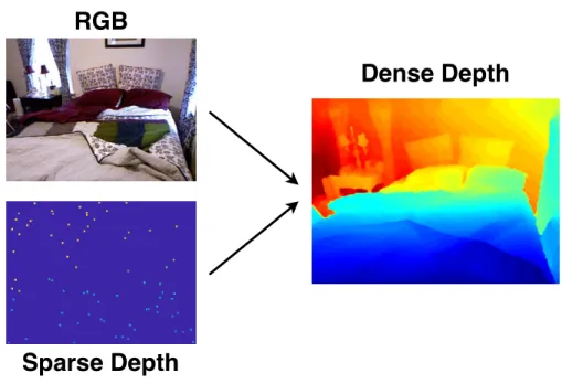
1-1 This thesis studies the single-view depth estimation estimation. The input includes a sparse depth image and optionally a color image. The goal is to reconstruct a complete, dense depth image. . . 22 1-2 Example of depth completion on lidar scans from Velodyne HDL-64. From

top to bottom: RGB image, raw lidar scans, and dense depth estimation from our method described in Chapter 3. . . 24 1-3 Example of depth completion on Kinect [1]. Using both (a) RGB and (b)

incomplete depth raw data produced by Kinect, a depth estimation algo-rithm can produce (c) enhanced depth image. . . 24 1-4 (a) RoboBees [2] are flapping-wing micro-robots without onboard sensing

capabilities. (b) Lidar-on-a-chip [3] is a new 3D Lidar with size smaller than a dime, but also produces low-resolution depth image. . . 25 1-5 Most state-of-the-art, real-time, visual SLAM algorithms only track and

triangulate a small number of pixels in the scene. Consequently, these al-gorithms only maintain a sparse 3D representation of the environment. A sparse map is not ideal for robot navigation. . . 26 1-6 An example of map densification using our method described in Chapter 3.

From left to right: (a) RGB, (b) sparse map, (c) prediction point cloud (cre-ated by stitching RGBd predictions from each frame), and (d) ground truth. 27 2-1 We show how to reconstruct an unknown depth signal (a) from a handful

of samples (b). Our reconstruction is shown in (c). Our results also apply to traditional stereo vision and enable accurate reconstruction (f) from few depth measurements (e) corresponding to the edges in the RGB image (d). Figures (a) and (d) are obtained from a ZED stereo camera. . . 33 2-2 (a) Example of 2D depth signal. Our goal is to reconstruct the full

sig-nal (black solid line) from sparse samples (red dots); (b) When we do not sample the corners and the neighboring points, (2.9) admits multiple mini-mizers, which obey the conditions of Proposition 14. . . 37 2-3 (a) Sampling corners and neighbors in 2D depth estimation guarantees

ex-act recovery of the true signal. (b) Sampling only the corners does not guar-antee, in general, that the solution of theℓ1-minimization, namely𝑧⋆, coin-cides with the true signal𝑧◇. . . 42 2-4 Examples of sign-consistent (shown in black) and sign-inconsistent (shown

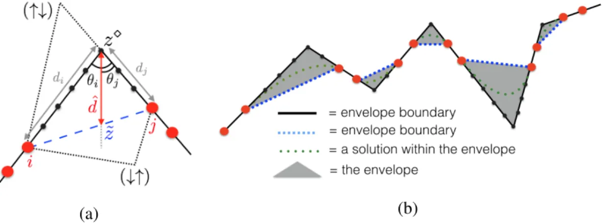
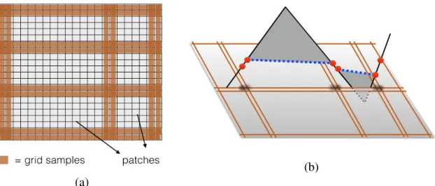
2-5 (a) Region between a pair of twin samples, with twin samples not including corners.𝑑𝑖and𝑑𝑗represent distances between samples and the intersection of two lines. The up and down arrows represent the change of slopes. (b) Given a set of noiseless twin samples, all possible optimal solutions in 2D are contained in the envelope shown in gray. . . 45 2-6 (a) Illustration of a grid sample set, along with 6 non-sampled patches in

white. (b) A cross section of the envelope in 3D. . . 46 2-7 A illustration of the active set _{𝒜 of samples in Proposition 19. The three}

corners, as well as the second sample from the right, are all within the active set. A measurement𝑦𝑖 is active if the reconstructed signal z hits the boundary of𝑦𝑖’s associated error bound. . . 48 2-8 (a) Illustration of the line segments (1)-(6) in Definition 22 with

intersec-tion. (b) Line segments (1)-(6) without intersecintersec-tion. (c) An example of 2D sign consistent𝜖-envelope. . . 50 2-9 A toy example illustrating that while a 2D lidar produces measurements at

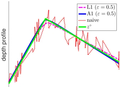
fixed angular resolution, the resulting Cartesian coordinates are not equally spaced, i.e.,∆𝑥1 ̸= ∆𝑥2. This occurs in both lidars and perspective cam-eras, hence motivating the introduction of the L1cart formulation. . . 54 2-10 An example of synthetic 2D signal and typical behavior of the compared

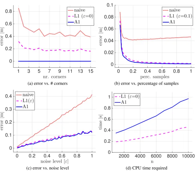
techniques, naive, L1, and A1, for noise level𝜀 = 0.5m. . . 58 2-11 (a) Estimation errors committed by A1, L1, and naive, for increasing

number of corners in the ground truth signal. A twin sample is acquired in each linear segment and measurements are noiseless. (b) Estimation er-rors from uniformly sampled noisy measurements, with increasing number of samples. (c) Estimation errors from uniformly sampled noisy measure-ments (5% of the depth data points) and increasing noise level. (d) CPU time required to solve L1 and A1 for increasing size 𝑛 of the 2D depth signal. . . 59 2-12 (a) Mapping using a conventional laser scanner, (b-c) Mapping using scans

reconstructed by naive and A1 using 10 depth measurements. . . 60 2-13 (a) Gazebo Simulated data. (b) ZED Stereo data. (c)-(d) Kinect data. . . 61 2-14 Comparison between three different objective functions, L1, L1diag, and

L1cart, on 10 benchmarking datasets. (a) constant in L1cart is chosen as𝛿 = 0.1m, (b) constant in L1cart is chosen as 𝛿 = 0.01m. . . 62 2-15 Trade-off between accuracy and speed for theNESTAsolver with different

parameter values 𝜇𝑓. As 𝜇𝑓 decreases, NESTA produces a more accurate solution at the cost of higher computational time. The error is computed as the average mismatch between theNESTAandcvx solutions. . . 64 2-16 Comparison betweenNESTA(𝜇𝑓 = 0.001) andcvx. Estimation errors and

timing are shown for (a-b) increasing number of samples, (c-d) increas-ing measurement noise, (e-f) increasincreas-ing size of the𝑁 _{× 𝑁 depth signals.}

NESTAachieves comparable reconstruction errors, while offering a signif-icant speedup. . . 65

2-17 The first row is an example of sparse depth reconstruction on Gazebo sim-ulated data: (a) RGB image, (b) uniformly drawn sparse samples, and (c) reconstruction using L1diag. The second row is an example on Kinect K1 data: (d) RGB image, (e) sparse samples on a grid, and (f) reconstruction using L1diag. . . 66 2-18 Qualitative results on Gazebo dataset: 3 examples of reconstructed depth

signals using the proposed approaches (L1, L1diag) and a naive linear interpolation (naive). For each example we show the reconstruction from 2% uniformly drawn depth measurements. We also show the reconstruc-tion for the case in which we can access the depth corresponding to (ap-pearance) edges in the RGB images. . . 67 2-19 Qualitative results on ZED: 3 examples of reconstructed depth signals

us-ing the proposed approaches (L1, L1diag) and a naive linear interpo-lation (naive). For each example we show the reconstruction from 2% uniformly drawn depth measurements. We also show the reconstruction for the case in which we can access the depth corresponding to (appearance) edges in the RGB images. . . 68 2-20 Reconstruction errors for increasing percentage of uniform samples, and

for different datasets. (a) and (b) are reconstructions on the Gazebo dataset, using noiseless and noisy (noise bounded by 𝜀 = 0.1m) samples, respec-tively. (c) reconstruction on the ZED dataset, (d) reconstruction on the K1 dataset. (e) comparison on all datasets. . . 70 2-21 Examples of reconstruction from 5% uniformly random samples on the

Middlebury disparity dataset, using 4 different algorithms: naive, L1diag, CSR [4], and WT+CT [5]. The proposed algorithm, L1diag, is able to pre-serve sharper boundaries and finer details, while not creating jagged edges as in naive. . . 71 2-22 Reconstructed depth profile of the “Art” image from the Middlebury dataset

from 5% uniform random measurements, visualized as point cloud. Red in-dicates errors and green highlights good reconstruction quality. In compar-ison against naive and WT+CT [5], L1diag produces the most complete structures with the least outliers. . . 72 2-23 Super-resolution depth imaging. The up-scale factor is 24.79 in this

exam-ple. . . 75 3-1 CNN architecture for NYU-Depth-v2 and KITTI datasets, respectively.

The network for KITTI has fewer layers and channels, since KITTI has a larger image size than NYU-Depth-v2 and thus demands higher mem-ory consumption. Cubes are feature maps, with dimensions represented as #features@height_{×width. The encoding layers in blue consist of a ResNet [6]} and a 3_{×3 convolution. The decoding layers in yellow are composed of 4} upsampling layers (UpProj) followed by a bilinear upsampling. . . 78 3-2 Predictions on NYU-Depth-v2. From top to bottom: (a) RGB images; (b)

RGB-based prediction; (c) d prediction with 200 and no RGB; (d) RGBd prediction with 200 sparse depth and RGB; (e) ground truth depth. . . 83

3-3 Impact of number of depth sample on the prediction accuracy on the NYU-Depth-v2 dataset. Left column: lower is better; right column: higher is better. 85 3-4 Impact of number of depth sample on the prediction accuracy on the KITTI

dataset. Left column: lower is better; right column: higher is better. . . 86 3-5 Application in sparse SLAM and visual inertial odometry (VIO) to create

dense point clouds from sparse landmarks. (a) RGB (b) sparse landmarks (c) ground truth point cloud (d) prediction point cloud, created by stitching RGBdpredictions from each frame. . . 87 3-6 An illustration of the self-supervised training framework, which requires

only a sequence of color images and sparse depth images. White rectangles are variables, red is the depth network to be trained, blue are deterministic computational blocks (without learnable parameters), and green are loss functions. . . 88 3-7 Comparison between different training methods (best viewed in color). The

photometric loss provides supervision at the top, where the semi-dense an-notation does not contain labels. . . 91 3-8 Prediction error against number of input depth samples, for both spatial

patterns (uniform random sub-sampling and Lidar scan lines). (a) When trained with semi-dense ground truth, the depth completion error decreases as a power function 𝑐𝑥𝑝 _{of the number of input depth measurements, for} some𝑐 > 0, 𝑝 < 0. (b) The self-supervised framework is effective with suf-ficiently many measurements (at least 4 scanlines, or the equivalent number of samples to 2 scanlines when input is uniformly sampled). . . 93 4-1 Recovery of the input latent code𝑧 from under-sampled measurements 𝑦 =

𝐴𝐺(𝑧) where 𝐴 is a sub-sampling matrix and 𝐺 is an expanding generative neural network. We prove that 𝑧 can be recovered with guarantees using simple gradient-descent methods under mild technical assumptions. Best viewed in color. . . 96 4-2 Illustration of a single transposed convolution operation.𝑓𝑖,𝑗 stands for𝑖𝑡ℎ

filter kernel for the𝑗𝑡ℎ _{input channel.𝑧 and 𝑥 denote the input and output} signals, respectively. (a) The standard transposed convolution represented as linear multiplication. (b) With proper row and column permutations, the permuted weight matrix has a repeating block structure. . . 100 4-3 Distribution of the kernel weights from every layer in a trained

convolu-tional generative network. The trained weights roughly follow a zero-mean gaussian distribution. . . 103 4-4 The landscape of the cost function𝐽(𝑧) for deconvolutional networks with

(a) ReLU, (b) Sigmoid, and (c) Tanh as activation functions, respectively. There exists a unique global minimum. . . 104 4-5 We demonstrate recovery of latent codes on a generative network trained

on the MNIST dataset. From top to bottom: ground truth output images; partial measurements with different sampling masks; reconstructed image using the recovered latent codes from partial measurements. The recovery of latent codes is exact using simple gradient descent. . . 105

4-6 recovery of latent codes on a generative network trained on the CelebA dataset. From top to bottom: ground truth output images; partial measure-ments with different sampling masks; reconstructed image using the recov-ered latent codes from partial measurements. The recovery of latent codes is exact using simple gradient descent. . . 106 A-1 Region between a pair of twin samples, with a twin sample including a corner.119 A-2 Example of matrix(∆T₎

ℳ and corresponding column partition(∆T)ℳ,𝑉, (∆T₎

ℳ,𝐻. . . 120 A-3 Illustration of the upper bound𝑧 of 2D sign consistent 𝜖-envelope for all¯

possible orientations of the line segments (1), (3) and (5) defined in Defini-tion 22. . . 125 B-1 Plot of function𝑔(_{·) defined in Section B.2 . . . 133}

List of Tables

2.1 Summary of the key theoretical results. . . 41 2.2 Reconstruction accuracy and computational time comparing naive, L1diag,

CSR [4], and WT+CT [5]. L1diag consistently outperforms all other methods in accuracy, and performs robustly even with aggressively low number of measurements. . . 73 2.3 Our proposed solution outperforms state-of-the-art deep-learning based method [7]

on the NYU test dataset. The input depth is sampled uniform randomly (1%) from the ground truth. . . 74 3.1 Evaluation of loss functions, upsampling layers and the first convolution

layer. RGBd has an average sparse depth input of 100 samples. (a) compar-ison of loss functions is listed in Row 1 - 3; (b) comparcompar-ison of upsampling layers is in Row 2 - 4; (c) comparison of the first convolution layers is in the 3 bottom rows. . . 80 3.2 Comparison with state-of-the-art on the NYU-Depth-v2 dataset. The values

are those originally reported by the authors in their respective paper . . . . 82 3.3 Comparison with state-of-the-art on the KITTI dataset. The Make3D values

are those reported in [8] . . . 82 3.4 Evaluation of the self-supervised framework on the validation set . . . 91 B.1 Summary of notation . . . 129

Chapter 1

Introduction

The recovery of scene geometry and 3D structure has long been one of the core problems in computer vision, robotics, and mapping. A significant amount of past efforts (namely multi-view geometry, Structure from Motion, and Simultaneous Localization and Map-ping) has been devoted on 3D reconstruction from multiple viewing angles. Orthogonally, other work (e.g., single-view metrology) has been focusing on estimating geometry from one single frame of sensor data. This dissertation fits into this line of research and studies the problem of single-view depth image estimation. Our goal is to estimate the 3D structure of a scene, represented as a depth image, based on incomplete depth samples (for instance, raw measurements from a low-resolution lidar sensor) captured at a single viewing angle. Specifically, we address the following question: is it possible to reconstruct a dense, com-plete depth image from sparse and incomcom-plete depth samples?

In general, the answer is negative since depth reconstruction from incomplete measure-ments is an ill-posed inverse problem, meaning there exists an infinite number of possible solutions. However, in this thesis, by posing proper modeling assumptions regarding the scene geometry, we are able to develop efficient computational algorithms for reconstruc-tion of the 3D structure. In particular, we propose 3 different algorithms for single-view depth estimation, each based on a different set of modeling assumptions. We empirically demonstrate their performance on real data, and provide conditions for exact reconstruction under rigorous proofs.

1.1

Overview of Depth Sensing Techniques

Depth sensing, which refers to measuring distances from a sensor to the surrounding en-vironments, is fundamental in robotics and computer vision. It is an essential compo-nent in many engineering applications, including mapping [9, 10, 11, 12, 13], localiza-tion [14, 15, 16], obstacle avoidance [17, 18], and etc. The measured depth also serves as part of the input to a variety of higher-level computer vision tasks, including object recognition [19, 20, 21], detection [22, 23, 24, 25, 26], segmentation [27, 28, 29, 30], and beyond.

Historically, depth sensing techniques have been a key driver in the development of robotics. For instance, in 1970s, Moravec [31] developed the first stereo vision system for

the Stanford Cart, which became the first mobile robot to navigate around simple polygo-nal objects over 20 meters. Over the period of 1980s to early 2000s, sonars and 2D lidars inspired a large number of pioneering work on robot navigation [32, 33] and SLAM (Si-multaneous Localization and Mapping) [34, 35, 36]. In 2007, Velodyne Acoustics released the HDL-64E [37], the first 3D lidar. It was mounted atop five of the six autonomous ve-hicles that competed in the 2007 DARPA Urban Challenge [38] as an essential component in their perception systems [39, 40, 41, 42]. 3D lidars remain crucial to most autonomous driving cars today, as well as in the foreseeable future. In 2010, Microsoft introduced the structured-light based depth sensor Kinect. Kinect provides high-frequency, accurate and dense depth measurements, enabling high-speed MAV (Micro Aerial Vehicle) flights in cluttered, GPS-denied environment [13].

1.1.1

Depth sensors and limitations

Mainstream depth sensing techniques include sonar (Sound Navigation and Ranging) [43], radar (Radio Detection and Ranging) [44, 45, 46], lidar (Light Detection and Ranging) [47, 48], as well as stereo vision [49, 50] and its variants (e.g., structured-light sensors such as Microsoft Kinect V1 [51]). However, these depth sensing techniques offer many short-comings. No existing depth sensors can attain both high RRA (Range, Resolution and Ac-curacy) and low SWaP (Size, Weight and Power). Such limitations render existing depth sensors unfit for a large number of hardware platforms, including miniaturized robots and embedded systems.

Sonar Sonars were motivated by the impressive echolocation capabilities of bats in us-ing sound for aerial navigation [52]. Specifically, an active sonar creates a pulse of sound and then measures the time difference between transmission and reception of the reflected pulse. The distance to an object can then be derived as the product of one-half of the round-trip time with the speed of sound. This method for measuring distances is called ToF (time-of-flight). A typically sonar produces only planar measurements [43]. Sonars suffer from poor directionality, frequent misreadings, and data corruption due to specular reflections. The use of a sonar range finder represents a worst-case scenario for robot localization [53]. Radar Radars were initially developed for military purposes during World War II. Later radars find highly diverse applications, including automotive collision avoidance [54] and power line detection [55]. Based on the same ToF strategy as sonars, radars obtain distance measurements by first emitting a signal (radio waves) and then measuring the round-trip time. In addition, if an object is moving towards or away from the radar, its speed can be inferred from the change of received radio wave frequency caused by the Doppler effect. Furthermore, radars are robust against environmental influences including extreme weather and change of temperatures and lighting conditions [56]. However, in order to ensure in-terference suppression, only a few antennas are used on a radar sensor and mechanical scanning is used to sweep across a fixed angular range [56]. The output radar image has a low resolution.

the measure the round-trip time of the reflected pulses. Most lidars on vehicles today obtain a wide field of view by rotating laser beams. 3D lidars available today are bulky, heavy, power-consuming, and cost-prohibitive1_{. In addition, lidar has its limitations in adverse} weather conditions, such as snow, rain, and fog [57]. Furthermore, they have a fixed angular resolution, and thus provide only sparse measurements for distant objects, as illustrated in Figure 1-2.

In order to address the current limitations, extensive efforts have been invested into the development of new lidar hardware. For instance, companies in the lidar space are compet-ing to produce compact, narrow field-of-view solid-state lidars2_{[59] as a complement to the} existing high-end, 360-degree lidar. Research and development work to create tiny lidars is also underway in academia. For example, Poulton et al. [3] are developing a lidar-on-a-chip system with a size smaller than a dime.

Stereo Vision Stereo vision extracts 3D information by comparing a pair of slightly different views of the same scene, similar to the way human eyes work. Typically, two horizontally displaced cameras are used for triangulation. A disparity image between these two cameras can be computed using either local comparison approaches [19, 60] or global methods [61, 62]. However, stereo vision is computationally demanding. It also requires a large baseline and sufficiently dense textures for accurate disparity inference. Furthermore, stereo vision faces the same difficulty with precipitation and obscurants as lidars [57]. Structured-light Sensors Structured-light-based depth sensors (e.g. Kinect) are variants of the traditional stereo cameras. Take Microsoft Kinect V1 for an example: instead of using two cameras, Kinect V1 uses an IR (infrared) projector and an IR camera for depth sensing. The IR projector emits a special dot pattern, which brings robustness in areas with poor visual texture [51]. However, Structured-light-based depth sensors can be sensitive to sunlights, and are range-limited by their projectors (typically no more than 10 meters).

1.2

The Single-View Depth Estimation Problem

The single-view depth estimation problem is illustrated in Figure 1-1. In this problem, the input to the system includes a sparse depth image and optionally a RGB image of the same scene. A sparse depth image is a depth image where only a small set of pixels are measured, whilst the other pixels are simply encoded as zeros (corresponding to no sensor measure-ments). Sparse depth images are typically found in lidar measurements, or 3D landmarks tracked in a SLAM algorithm. The goal of is to predict a complete and dense depth image of the scene, given only the incomplete sensor measurements and information.

In particular, the problem is often dubbed depth completion or depth inpainting when the input includes sparse depth (with or without color). In comparison. when only a color image is available, the problem is often referred to as depth prediction. In this thesis, we focus on the depth completion problem, since in robotic applications it is relatively easy to

1_{The top-of-the-range 3D LiDARs cost up to $75,000 per unit.}

2_{Solid-state lidars are single-chip lidars with no moving parts. They rely on optical phased arrays for}

Figure 1-1: This thesis studies the single-view depth estimation estimation. The input in-cludes a sparse depth image and optionally a color image. The goal is to reconstruct a complete, dense depth image.

obtain sparse depth samples, either from a low-resolution depth sensors or from triangula-tions due to motriangula-tions.

1.2.1

Depth Image Representation

A depth image encodes the geometry information of the scene in the format of an image. A depth image is formed by projecting a 3D world point 𝑃 = (𝑋, 𝑌, 𝑍) into the image plane using a perspective transformation. The value of each depth pixel is simply𝑍 (i.e., the distance of 𝑃 along the optical axis). This image formation process can be modeled as a typical pinhole camera. Some alternative encoding of geometry include inverse depth representation (i.e., each pixel stores 1/𝑍 rather than 𝑍), or disparity between a pair of stereo cameras. Since there is no clear advantage of one representation over another, we adopt the linear representation𝑍 throughout this thesis for consistency.

1.2.2

Problem Formulation

Let𝑍 ∈ (0, ∞)ℎ×𝑤_{denote the target ground truth signal (a 2D depth image of heightℎ and} width𝑤), which we do not have direct access to. Instead, we only observe a sparse depth image𝑌 , given some sampling pattern known a priori. Consequently, the depth completion problem can be formally stated as follows.

Problem 1 (Matrix form). Find the target depth signal𝑍, given both the binary sampling mask𝐵 _{∈ {0, 1}}ℎ×𝑤 _{and the sparse depth measurements}

where𝐸 _{∈ R}ℎ×𝑤 represents unknown measurement noise (unless stated otherwise), and_∘ is the Hadamard product (i.e., element-wise product) between two matrices.

Alternatively, we can rephrase the same problem in matrix-vector multiplication form. Let𝑦_{∈ (0, ∞)}𝑚_{be a vector that includes all the𝑚 samples (i.e., all zeros in 𝑌 have been} excluded), then Problem 1 can be rewritten as

Problem 2 (Matrix-vector form). Find the target depth signal 𝑍, given both the sub-sampling matrix𝐴∈ {0, 1}𝑚×(ℎ*𝑤)_{and the sparse depth measurements}

𝑦 = 𝐴_{· vec(𝑍) + 𝜂,} (1.2)

where𝜂∈ R𝑚_{represents unknown measurement noise (unless stated otherwise), and vec()} is the vectorization operation.

Note that Problem 1 and Problem 2 are equivalent statements of the same problem this dissertation studies. They both represent a mathematical abstraction of the depth recon-struction problem, which can be application- and sensor-dependent in practice.

1.3

Application Areas

In this section we give a brief overview of some use cases of single-view depth estima-tion. In particular, we will look at depth sensor enhancement, hardware simplification and miniaturization, as well as sparse map densification.

1.3.1

Depth Sensor Enhancement

Existing depth sensors are considered to be low-resolution and noisy, as is discussed in Sec-tion 1.1.1. The single-view depth estimaSec-tion problem this dissertaSec-tion studies can enhance the quality of depth images captured by such depth sensors. For instance, lidar (Light De-tection and Ranging) produces only sparse measurements, see Figure 1-2. Similarly, Kinect generates depth maps with many missing pixels, see Figure 1-3(b), due to occlusions and other factors.

The incomplete raw depth data can lead to computational challenges and lower accuracy for high-level algorithms in the data processing pipeline. Therefore, depth completion and inpainting is usually required as a pre-processing step.

1.3.2

Hardware Simplification and Miniaturization

Another motivation for this thesis project is to enable onboard sensing and navigation ca-pabilities for miniaturized robotic systems. Recent years have witnessed a growing in-terest towards miniaturized robots, for instance the RoboBee [63], Piccolissimo [64], the DelFly [65, 66], the Black Hornet Nano [67], Salto [68]. These robots are usually palm-sized (or even smaller), can be deployed in large volumes, and provide a new perspective on societally relevant applications, including artificial pollination, environmental monitoring,

Figure 1-2: Example of depth completion on lidar scans from Velodyne HDL-64. From top to bottom: RGB image, raw lidar scans, and dense depth estimation from our method described in Chapter 3.

(a) rgb (b) Kinect raw data (c) completed data

Figure 1-3: Example of depth completion on Kinect [1]. Using both (a) RGB and (b) in-complete depth raw data produced by Kinect, a depth estimation algorithm can produce (c) enhanced depth image.

and disaster response. Despite the rapid development and recent success in control, actua-tion, and manufacturing of miniature robots, on-board sensing and perception capabilities for such robots remain a relatively unexplored, challenging open problem. These small platforms have extremely limited payload, power, and on-board computational resources, thus preventing the use of standard sensing and computation paradigms.

(a) RoboBees (b) lidar on a chip

Figure 1-4: (a) RoboBees [2] are flapping-wing micro-robots without onboard sensing ca-pabilities. (b) Lidar-on-a-chip [3] is a new 3D lidar with size smaller than a dime, but also produces low-resolution depth image.

In the last two decades, a large body of robotics research focused on the development of techniques to perform inference from data produced by “information-rich” sensors (e.g., high-resolution cameras, 2D and 3D laser scanners). A variety of approaches has been proposed to perform geometric reconstruction using these sensors, for instance see [69, 70, 71] and the references therein. On the other extreme of the sensor spectrum, applications and theories have been developed to cope with the case of minimalistic sensing [72, 73, 74, 75]. In this latter case, the sensor data is usually not metric (i.e., the sensor cannot measure distances or angles) but instead binary in nature (e.g., binary detection of landmarks), and the goal is to infer only the topology of the (usually planar) environment rather than its geometry. This work studies a relatively unexplored region between these two extremes of the sensor spectrum.

This thesis complements recent work on hardware and sensor design, including the de-velopment of lightweight, small-sized depth sensors. For instance, a number of ultra-tiny laser range sensors are being developed as research prototypes (e.g., the dime-sized, 20-gram laser of [76], and an even smaller lidar-on-a-chip system with no moving parts [77]), while some other distance sensors have already been released to the market (e.g., the Ter-aRanger’s single-beam, 8-gram distance sensor [78], and the LeddarVu’s 8-beam, 100-gram laser scanner [79]). These sensors provide potential hardware solutions for sensing on micro (or even nano) robots. Although these sensors meet the requirements of payload and power consumption of miniature robots, they only provide very sparse and incomplete depth data, in the sense that the raw depth measurements are extremely low-resolution (or even provide only a few beams). In other words, the output of these sensors cannot be uti-lized directly in high-level tasks (e.g., object recognition and mapping), and the need to

reconstruct a complete depth profile from such sparse data arises.

1.3.3

Sparse Map Densification

In many robotic navigation problems, Simultaneous Localization and Mapping (SLAM) is a critical task of the system. SLAM provides not only the position of the robot, but also a map of the surrounding environments. Most state-of-the-art, real-time, visual SLAM algorithms (e.g., ORB-SLAM [80], LSD-SLAM [81], PTAM [82, 83]) only track and trian-gulate a small number of pixels in the scene. Consequently, these algorithms only maintain a sparse 3D representation of the environment, see Figure 1-5. However, such sparse maps are far from ideal, because it provides only partial information regarding the scene geome-try.

(a) PTAM [82, 83] (b) LSD-SLAM [81]

Figure 1-5: Most state-of-the-art, real-time, visual SLAM algorithms only track and trian-gulate a small number of pixels in the scene. Consequently, these algorithms only maintain a sparse 3D representation of the environment. A sparse map is not ideal for robot naviga-tion.

As a remedy, depth estimation techniques can be applied as a downstream component of the SLAM algorithm. Specifically, as post-process step, depth estimation algorithms create a dense representation of the environment from the sparse map tracked by SLAM. This solution creates a map of significantly higher density, without incurring any extra computational overhead in the SLAM algorithm. An example is demonstrated in Figure 1-6. The estimated dense representation is not only visually more comprehensible, but also improves the safety and efficiency of robot navigation missions.

(a) RGB (b) sparse map (c) densified map (d) ground truth Figure 1-6: An example of map densification using our method described in Chapter 3. From left to right: (a) RGB, (b) sparse map, (c) prediction point cloud (created by stitching RGBdpredictions from each frame), and (d) ground truth.

1.4

Literature Review

This thesis intersects several lines of research across fields. In particular, the most rele-vant topics include depth image inpainting, super-resolution and prediction. RGB image inpainting also shares some similarities to the depth reconstruction problem. In addition, this dissertation also relates to 3D reconstruction problems such as structure from motion.

1.4.1

Depth Image Inpainting and Completion

Depth completion[84, 85] and depth inpainting [86] refer to the problem of filling in miss-ing pixels in a depth image. Both two terms are used interchangeably in some context. The depth completion problem is typically sensor- and input-dependent. Consequently, the problem faces vastly different levels of algorithmic difficulty, under different input modal-ities (with color images for guidance [87, 88] vs. without [89]) and depth densmodal-ities (dense depth input [85, 87, 90] vs. sparse depth measurements [7, 91]).

High-density Input Depth completion for structured light sensor (e.g., Microsoft Kinect) [1] is more often referred to as depth inpainting [86], or depth enhancement [85, 87, 90] when noise is taken into account. The task is to fill in small missing holes in the relatively dense depth images. This problem is relatively easy, since a large portion of pixels (typically over 80%) are observed. Consequently, even simple filtering-based methods [85] can provide good results.

Sparse Input In comparison, the completion problem becomes significantly more chal-lenging with a low depth density (e.g., below 5%), which is the scenario that we would like to study in this thesis. For instance, one application is to create a dense disparity map from sparse triangulated feature correspondences in stereo vision [4, 5]. [4] exploit the sparsity of the disparity maps in the Wavelet domain. The dense reconstruction problem is then posed as an optimization problem that simultaneously seeks a sparse coefficient vector in the Wavelet domain while preserving image smoothness. They also introduce a conjugate subgradient method for the resulting large-scale optimization problem. Liu et al. [5] empir-ically show that a combined dictionary of wavelets and contourlets produces a better sparse

representation of disparity maps, leading to more accurate reconstruction.

Another application is lidar depth completion. For instance, in the KITTI dataset [89], the projected depth measurements from a Velodyne lidar onto the camera image space account for only roughly 4% of all pixels. Depth completion using these sparse lidar mea-surements has attracted a significant amount of recent interest. Ku et al. [92] developed a simple and fast interpolation-based algorithm that runs on CPUs. Uhrig et al. [89] proposed sparse convolution, a variant of regular convolution operations with input normalizations, to address data sparsity in neural networks. Eldesokey et al. [93] improved the normalized convolution for confidence propagation. Chodosh et al. [94] incorporated the traditional dictionary learning with deep learning into a single framework for depth completion. Ca-dena et al. [95] developed a multi-modal auto-encoder to learn from three input modalities, including RGB, depth, and semantic labels. In their experiments, Cadena et al. [95] used sparse depth on extracted FAST corner features as part of the input to the system to pro-duce a low-resolution depth prediction. The accuracy was comparable to using RGB alone. Liao et al. [96] studied the use of a 2D laser scanner mounted on a mobile ground robot to provide an additional reference depth signal as input and obtained higher accuracy than using RGB images alone.

1.4.2

Depth Super-resolution

Both the depth completion and inpainting problems also find close connection to depth super-resolution[97, 98, 99, 100, 101, 102]. Depth super-resolution is the problem of cre-ating a higher resolution depth image using only a low-resolution depth image as input, and can be treated as a special case of depth completion and inpainting where the sparse depth input has a grid-structure. Hui et al. [103] propose a Mult-Scale Guided convolution network (MSG-Net), which upsamples the high-frequency components of a low-resolution depth image progressively. The high-resolution depth image is reconstructed by merging the upsampled high-frequency component with the low-frequency counterpart. Uhrig et al. [89] propose a new convolution operation which normalizes the output with the number of non-zero input pixels, and show experimentally that this operation exhibit high level of sparsity-invariance.

Limitations Prior work in depth completion mostly focuses on the high-density regime. However, the problem becomes significantly more challenging with a low-density, sparse input. Depth completion with sparse input has traditionally received relatively little atten-tion due to its complexity, but has started to attract attenatten-tions since very recently. Most of the existing efforts are on an ad-hoc basis, and lack performance guarantees.

1.4.3

Depth Prediction from Color Images

Color-based depth image prediction, which refers to the inference of 3D depth information from a single 2D color image, is an active research area in computer vision and robotics. Early Work Early works on depth estimation using RGB images usually relied on hand-crafted features and probabilistic graphical models. For instance, Saxena et al. [104]

esti-mated the absolute scales of different image patches and inferred the depth image using a Markov Random Field model. Non-parametric approaches [105, 106, 107, 108] were also exploited to estimate the depth of a query image by combining the depths of images with similar photometric content retrieved from a database.

Deep-Learning Approaches The state-of-the-art RGB-based depth prediction methods exclusively use deep-learning based methods to train a convolution neural network using large-scale datasets [109, 110, 111]. Eigen et al. [8] suggest a two-stack convolutional neu-ral network (CNN), with one predicting the global coarse scale and the other refining local details. Eigen and Fergus [110] further incorporate other auxiliary prediction tasks into the same architecture. Liu et al. [109] combined a deep CNN and a continuous conditional random field, and attained visually sharper transitions and local details. Laina et al. [111] developed a deep residual network based on the ResNet [6] and achieved higher accuracy than [109, 110]. Semi-supervised [112] and unsupervised learning [113, 114, 115] setups have also been explored for disparity image prediction. For instance, Godard et al. [115] formulated disparity estimation as an image reconstruction problem, where neural networks were trained to warp left images to match the right. Mancini et al. [116] proposed a CNN that took both RGB images and optical flow images as input to predict distance.

Self-supervised Frameworks Most learning-based work relied on pixel-level ground truth depth training. However, ground truth depth is generally not available and cannot be manually annotated. To address such difficulties, recent focus has shifted towards seeking other supervision signals for training. For instance, Zhou et al. [113] developed an unsu-pervised learning framework for simultaneous estimation of depth and ego-motion from a monocular camera, using photometric loss as a supervision. However, the depth estimation is only up-to-scale. Mahjourian et al. [117] improved the accuracy by using 3D geometric constraints, and Yin and Shi [118] extended the framework for optical flow estimation. Li et al. [119] recovered the absolute scale by using stereo image pairs.

Limitations However, the accuracy and reliability of the above methods is still far from being practical, especially for robotic tasks that demand high precision and robust-ness. The state-of-the-art learning-based methods produce an average error (measured by the root mean squared error) of over 50cm in indoor scenarios (e.g., on the NYU Depth Dataset [30]). Such methods perform even worse outdoors, with at least 4 meters of aver-age error on Make3D [120] and KITTI datasets [121].

1.4.4

Structure from Motion and SLAM

The geometric structure of a scene can be recovered by using triangulation from different views, when the scene contains sufficient textures or features and the environment is static. A survey for the current state of SLAM is presented in [122]. However, in many practical applications, the sensor might be static with no motion, or there exist transient and dynamic objects. Therefore, structure from motion might not always be applicable.

The idea of leveraging priors on the structure of the environment to improve or enable geometry estimation has been investigated in early work in computer vision for

single-view 3D reconstruction and feature matching [123, 124]. Early work by [125] addresses Structure from Motionby assuming the environment to be piecewise planar. More recently, [126] propose an approach to speed-up stereo reconstruction by computing the disparity at a small set of pixels and considering the environment to be piecewise planar elsewhere. [127] combine live dense reconstruction with shape-priors-based 3D tracking and recon-struction. [128] propose a regularization based on the structure tensor to better capture the local geometry of images. [99] produce high-resolution depth maps from subsampled depth measurements by using segmentation based on both RGB images and depth samples. [129] compute a dense depth map from a sparse point cloud.

1.4.5

Color Image Inpainting

The problem we address also shares some similarities with the image denoising prob-lem as well as the inpainting probprob-lem [130, 131] (where the goal is to fill in missing pixels in a color image). Some of the work include on exemplar-based inpainting [132], diffusion methods [133], total variation minimization [134, 135], and deep neural net-works [136, 137]. However, the difference in sensor modalities (RGB vs. depth) results in opportunities to better explore the underlying structure of depth images. However, RGB images have a different underlying distribution than depth images, and thus color inpainting is not the same problem as depth completion. Specifically, textures are independent of geo-metric structures of objects, so a simple planar objects can display colorful patterns whilst a complex shape might have constant colors. Therefore, a naive application of algorithms designed for color images will not produce optimal accuracy for depth estimation.

1.5

Statement of Contributions

This thesis addresses the following question: is it possible to reconstruct a complete depth signal from sparse and incomplete depth samples?In particular, we study the depth recon-struction problem from both the algorithmic and computational perspectives, and develop algorithms for the depth completion problem especially when the depth input is highly sparse. Numerous contributions arise from this study.

The first contribution is an algorithm for efficient reconstruction of 3D planar surfaces. This algorithm assumes that the 3D structure is piecewise-planar, and thus the second-order derivatives of the depth image are sparse. We develop a linear programming problem for recovery of the 3D surfaces under such assumptions, and provide conditions under which the reconstruction is exact. This method requires no learning, but still outperforms deep-learning-based methods under certain conditions.

The second contribution is a deep regression network and a self-supervised learning framework. We formulate the depth completion problem as a pixel-level regression prob-lem and solve it by training a neural network. Additionally, to address the difficulty in gath-ering ground truth annotations for depth data, we develop a self-supervised framework that trains the regression network by enforcing temporal photometric consistency, using only raw RGB and sparse depth data. The supervised method achieves state-of-the-art accuracy, and the self-supervised approach attains a lower but comparable accuracy.

Our third contribution is a two-stage algorithm for a broad class of inverse problems (e.g., depth completion and image inpainting). We assume that the target image is the out-put of a generative neural network, and only a subset of the outout-put pixels is observed. The goal is to reconstruct the unseen pixels based on the partial samples. Our proposed al-gorithm first recovers the corresponding low-dimensional input latent vector using simple gradient-descent, and then reconstructs the entire output with a single forward pass. We provide conditions under which the proposed algorithm achieves exact reconstruction, and empirically demonstrate the effectiveness of such algorithms on real data.

1.6

Organization

This dissertation consists of three contributed algorithms for solving the single-view depth estimation problem. There is a wide spectrum of possible angles to attack the problem, ranging from pure model-based approach to completely data-driven approach. In this dis-sertation, we provide three different approaches on the spectrum, where each algorithm is based on a different set of modeling assumptions.

In particular, Chapter 2 presents our first contributed algorithm for depth reconstruction from sparse measurements. This is a model-based algorithm, which is developed based on the assumption that the scene contains mostly planar surfaces and requires solving a simple linear programming optimization problem. In Chapter 3, we present the second contribu-tion – a data-driven deep regression approach based on neural networks and self-supervised learning. In Chapter 4, we introduce the third algorithm, which lies between the first two contributions in terms of the spectrum of methods. Specifically, it is based on generative network inversion. We assume that the target image is the output of a given generative neural network, and the missing pixels can be recovered by inverting the network and find-ing the low-dimensional latent representation. This algorithm achieves exact reconstruction under our assumptions. At the end, in Chapter 5, we provide a summary of the results pre-sented in this dissertation and outline future research directions.

Chapter 2

Planar Surface Reconstruction

In this chapter1_{, we present our first set of contributions – a collection of novel algorithms} (and the corresponding theoretical foundations) to reconstruct a depth signal (i.e., a laser scan in 2D, or a depth image in 3D, see Figure 2-1) from sparse and incomplete depth measurements. These algorithms are pure model-based, where we make strong assumptions on the scene geometry without tuning any parameters based on data.

(a) ground truth (b) 2% grid samples (c) reconstruction

(d) RGB image (e) sample along edges (f) reconstruction

Figure 2-1: We show how to reconstruct an unknown depth signal (a) from a handful of samples (b). Our reconstruction is shown in (c). Our results also apply to traditional stereo vision and enable accurate reconstruction (f) from few depth measurements (e) correspond-ing to the edges in the RGB image (d). Figures (a) and (d) are obtained from a ZED stereo camera.

Specifically, we assume that a structured environment (e.g., indoor, urban scenarios) where the depth data exhibits some regularity. For instance, man-made environments are

characterized by the presence of many planar surfaces and a few edges and corners. This chapter shows how to leverage this regularity to recover a depth signal from a handful of sensor measurements. Our overarching goal is two-fold: to establish theoretical conditions under which depth reconstruction from sparse and incomplete measurements is possible, and to develop practical inference algorithms for depth estimation.

Our first contribution, presented in Section 2.3, is a general formulation of the depth estimation problem. Here we recognize that the “regularity” of a depth signal is captured by a specific function (the ℓ0-norm of the 2nd-order differences of the depth signal). We also show that by relaxing the ℓ0-norm to the (convex)ℓ1-norm, our problem falls within the cosparsity model in compressive sensing (CS). We review related work and give pre-liminaries on CS in Section 2.1 and Section 2.2.

The second contribution, presented in Section 2.4, is the derivation of theoretical con-ditions for depth recovery. In particular, we provide concon-ditions under which reconstruction of a signal from incomplete measurements is possible, investigate the robustness of depth reconstruction in the presence of noise, and provide bounds on the reconstruction error. Contrary to the existing literature in CS, our conditions are geometric (rather than alge-braic) and provide actionable information to guide sampling strategy.

Our third contribution, presented in Section 2.5, is algorithmic. We discuss practical al-gorithms for depth reconstruction, including different variants of the proposed optimization-based formulation, and solvers that enable fast depth recovery. In particular, we discuss the application of a state-of-the-art solver for non-smooth convex programming, called

NESTA[138].

Our fourth contribution, presented in Section 2.6, is an extensive experimental evalu-ation, including Monte Carlo runs on simulated data and testing with real sensors. The experiments confirm our theoretical findings and show that our depth reconstruction ap-proach is extremely resilient to noise and works well even when the regularity assumptions are partially violated. We discuss many applications for the proposed approach. Besides our motivating scenario of navigation with miniaturized robots, our approach finds application in several endeavors, including data compression and super-resolution depth estimation.

2.1

Related Work on Compressive Sensing

Our work is related to the literature on compressive sensing [139, 140, 141, 142] (CS). While Shannon’s theorem states that to reconstruct a signal (e.g., a depth signal) we need a sampling rate (e.g., the spatial resolution of our sensor) which must be at least twice the maximum frequency of the signal, CS revolutionized signal processing by showing that a signal can be reconstructed from a much smaller set of samples if it is sparse in some do-main. CS mainly invokes two principles. First, by inserting randomness in the data acqui-sition, one can improve reconstruction. Second, one can useℓ1-minimization to encourage sparsity of the reconstructed signal. Since its emergence, CS impacted many research areas, including image processing (e.g., inpainting [143], total variation minimization [144]), data compression and 3D reconstruction [145, 146, 147], tactile sensor data acquisition [148], inverse problems and regularization [149], matrix completion [150], and single-pixel imag-ing techniques [151, 152, 153]. While most of the CS literature assumes that the original

signal 𝑧 is sparse in a particular domain, i.e., 𝑧 = 𝐷𝑥 for some matrix 𝐷 and a sparse vector𝑥 (this setup is usually called the synthesis model), very recent work considers the case in which the signal becomes sparse after a transformation is applied (i.e., given a matrix𝐷, the vector 𝐷𝑧 is sparse). The latter setup is called the analysis (or cosparsity) model [154, 155]. An important application of the analysis model in compressive sens-ing is total variation minimization, which is ubiquitous in image processsens-ing [144, 156]. In a hindsight we generalize total variation (which applies to piecewise constant signals) to piecewise linear functions.

2.2

Preliminaries and Notation

We use uppercase letters for matrices, e.g., 𝐷 ∈ R𝑝×𝑛_{, and lowercase letters for vectors} and scalars, e.g, 𝑧 _{∈ R}𝑛 _{and 𝑎 ∈ R. Sets are denoted with calligraphic fonts, e.g., ℳ.} The cardinality of a set _{ℳ is denoted with |ℳ|. For a set ℳ, the symbol ℳ denotes} its complement. For a vector 𝑧 ∈ R𝑛 _{and a set of indices ℳ ⊆ {1, . . . , 𝑛}, 𝑧}

ℳ is the sub-vector of 𝑧 corresponding to the entries of 𝑧 with indices in _{ℳ. In particular, 𝑧}𝑖 is the𝑖-th entry. The symbols 1 (resp. 0) denote a vector of all ones (resp. zeros) of suitable dimension.

The support set of a vector is denoted with

supp(𝑧) =_{{𝑖 ∈ {1, . . . , 𝑛} : 𝑧}𝑖 ̸= 0}.

We denote with_‖𝑧‖2 the Euclidean norm and we also use the following norms: ‖𝑧‖∞ =. max 𝑖=1,...,𝑛 |𝑧𝑖| (ℓ∞norm) (2.1) ‖𝑧‖1 =. ∑︁ 𝑖=1,...,𝑛 |𝑧𝑖| (ℓ1 norm) (2.2) ‖𝑧‖0 =. |supp(𝑧)| (ℓ0pseudo-norm) (2.3)

Note that_‖𝑧‖0 is simply the number of nonzero elements in𝑧. The sign vector sign(𝑧) of 𝑧 _{∈ R}𝑛_{is a vector with entries:}

sign(𝑧)𝑖 =. ⎧ ⎨ ⎩ +1 if 𝑧𝑖 > 0 0 if 𝑧𝑖 = 0 −1 if 𝑧𝑖 < 0

For a matrix𝐷 and an index set_{ℳ, let 𝐷ℳ}denote the sub-matrix of𝐷 containing only the rows of 𝐷 with indices inℳ; in particular, 𝐷𝑖 is the 𝑖-th row of 𝐷. Similarly, given two index sets_{ℐ and 𝒥 , let 𝐷ℐ,𝒥} denote the sub-matrix of𝐷 including only rows inℐ and columns in_{𝒥 . Let I denote the identity matrix. Given a matrix 𝐷 ∈ R}𝑝×𝑛, we define the following matrix operator norm

‖𝐷‖∞→∞ = max.

In the rest of the chapter we use the cosparsity model in CS. In particular, we assume that the signal of interest is sparse under the application of an analysis operator. The fol-lowing definitions formalize this concept.

Definition 1 (Cosparsity). A vector𝑧 _{∈ R}𝑛_{is said to becosparse with respect to a matrix} 𝐷_{∈ R}𝑝×𝑛_{if‖𝐷𝑧‖}

0 ≪ 𝑝.

Definition 2 (𝐷-support and 𝐷-cosupport). Given a vector 𝑧 ∈ R𝑛 _{and a matrix 𝐷 ∈} R𝑝×𝑛, the𝐷-support of 𝑧 is the set of indices corresponding to the nonzero entries of 𝐷𝑧, i.e.,_{ℐ = supp(𝐷𝑧). The 𝐷-cosupport 𝒥 is the complement of ℐ, i.e., the indices of the zero} entries of𝐷𝑧.

2.3

Problem Formulation

Our goal is to reconstruct 2D depth signals (i.e., a scan from a 2D laser range finder) and 3D depth signals (e.g., a depth image produced by a Kinect or a stereo camera) from partial and incomplete depth measurements. In this section we formalize the depth reconstruction problem, by first considering the 2D and the 3D cases separately, and then reconciling them under a unified framework.

2.3.1

2D Depth Reconstruction

In this section we discuss how to recover a 2D depth signal 𝑧◇ _{∈ R}𝑛_{. One can imagine} that the vector 𝑧◇ includes (unknown) depth measurements at discrete angles; this is what a standard planar range finder would measure.

In our problem, due to sensing constraints, we do not have direct access to 𝑧◇_{, and we} only observe a subset of its entries. In particular, we measure

𝑦 = 𝐴𝑧◇+ 𝜂 (sparse measurements) (2.4)

where the matrix 𝐴 ∈ R𝑚×𝑛 _{with 𝑚 ≪ 𝑛 is the measurement matrix, and 𝜂 represents} measurement noise. The structure of𝐴 is formalized in the following definition.

Definition 3 (Sample set and sparse sampling matrix). A sample set_{ℳ ⊆ {1, . . . , 𝑛} is} the set of entries of the signal that are measured. A matrix𝐴 ∈ R𝑚×𝑛_{is called a(sparse)} sampling matrix (with sample set_{ℳ), if 𝐴 = Iℳ}.

Recall thatI_ℳis a sub-matrix of the identity matrix, with only rows of indices in_{ℳ. It} follows that𝐴𝑧 = 𝑧_ℳ, i.e., the matrix𝐴 selects a subset of entries from 𝑧. Since 𝑚≪ 𝑛, we have much fewer measurements than unknowns. Consequently,𝑧◇_{cannot be recovered} from𝑦, without further assumptions.

In this chapter we assume that the signal 𝑧◇ is sufficiently regular, in the sense that it contains only a few “corners”, e.g., Figure 2-2(a). Corners are produced by changes of slope: considering 3 consecutive points at coordinates(𝑥𝑖−1, 𝑧𝑖−1), (𝑥𝑖, 𝑧𝑖), and (𝑥𝑖+1, 𝑧𝑖+1),2

2_{Note that𝑥 corresponds to the horizontal axis in Figure 2-2(a), while the depth 𝑧 is shown on the vertical}

(a) (b)

Figure 2-2: (a) Example of 2D depth signal. Our goal is to reconstruct the full signal (black solid line) from sparse samples (red dots); (b) When we do not sample the corners and the neighboring points, (2.9) admits multiple minimizers, which obey the conditions of Propo-sition 14. there is a corner at𝑖 if 𝑧𝑖+1− 𝑧𝑖 𝑥𝑖+1− 𝑥𝑖 − 𝑧𝑖− 𝑧𝑖−1 𝑥𝑖− 𝑥𝑖−1 ̸= 0. (2.5) In the following we assume that𝑥𝑖−𝑥𝑖−1 = 1 for all 𝑖: this comes without loss of generality since the full signal is unknown and we can reconstruct it at arbitrary resolution (i.e., at arbitrary𝑥); hence (2.5) simplifies to 𝑧𝑖−1− 2𝑧𝑖+ 𝑧𝑖+1̸= 0. We formalize the definition of “corner” as follows.

Definition 4 (Corner set). Given a 2D depth signal𝑧 _{∈ R}𝑛_{, thecorner set𝒞 ⊆ {2, . . . , 𝑛−} 1_{} is the set of indices 𝑖 such that 𝑧}𝑖−1− 2𝑧𝑖 + 𝑧𝑖+1 ̸= 0.

Intuitively,𝑧𝑖−1− 2𝑧𝑖+ 𝑧𝑖+1 is the discrete equivalent of the 2nd-order derivative at𝑧𝑖. We call𝑧𝑖−1−2𝑧𝑖+𝑧𝑖+1the curvature at sample𝑖: if this quantity is zero, the neighborhood of𝑖 is flat (the three points are collinear); if it is negative, the curve is locally concave; if it is positive, it is locally convex. To make notation more compact, we introduce the 2nd-order difference operator: 𝐷=. ⎡ ⎢ ⎢ ⎢ ⎣ 1 −2 1 0 . . . 0 0 1 _{−2 1} . . . 0 .. . 0 . .. ... ... 0 0 . . . 0 1 _{−2 1} ⎤ ⎥ ⎥ ⎥ ⎦ ∈ R(𝑛−2)×𝑛 (2.6)

Then a signal with only a few corners is one where𝐷𝑧◇ _{is sparse. In fact, theℓ}

0-norm of𝐷𝑧◇ counts exactly the number of corners of a signal:

‖𝐷𝑧◇‖0 =|𝒞| (# of corners) (2.7)

where_{|𝒞| is the number of corners in the signal.}

When operating in indoor environments, it is reasonable to assume that 𝑧◇ has only a few corners. Therefore, we want to exploit this regularity assumption and the partial measurements 𝑦 in (2.4) to reconstruct 𝑧◇_{. Let us start from the noiseless case in which} 𝜂 = 0 in (2.4). In this case, a reasonable way to reconstruct the signal 𝑧◇ is to solve the

following optimization problem: min

𝑧 ‖𝐷𝑧‖0 s.t.𝐴𝑧 = 𝑦 (2.8)

which seeks the signal 𝑧 that is consistent with the measurements (2.4) and contains the smallest number of corners. Unfortunately, problem (2.8) is NP-hard due to the nonconvex-ity of theℓ0(pseudo) norm. In this work we study the following relaxation of problem (2.8):

min

𝑧 ‖𝐷𝑧‖1 s.t.𝐴𝑧 = 𝑦 (2.9)

which is a convex program (it can be indeed rephrased as a linear program), and can be solved efficiently in practice. Section 2.4 provides conditions under which (2.9) recovers the solution of (2.8). Problem (2.9) falls in the class of the cosparsity models in CS [155].

In the presence of bounded measurement noise (2.4), i.e.,_{‖𝜂‖∞ ≤ 𝜀, the ℓ}1-minimization problem becomes:

min

𝑧 ‖𝐷𝑧‖1 s.t. ‖𝐴𝑧 − 𝑦‖∞ ≤ 𝜀 (2.10)

Note that we assume that theℓ∞norm of the noise𝜂 is bounded, since this naturally reflects the sensor model in our robotic applications (i.e., bounded error in each laser beam). On the other hand, most CS literature considers theℓ2norm of the error to be bounded and thus obtains an optimization problem with theℓ2 norm in the constraint. The use of theℓ∞norm as a constraint in (2.10) resembles the Dantzig selector of Candes and Tao [157], with the main difference being the presence of the matrix𝐷 in the objective.

2.3.2

3D Depth Reconstruction

In this section we discuss how to recover a 3D depth signal𝑍◇ _{∈ R}𝑟×𝑐 _{(a depth map, as the} one in Figure 2-1(a)), using incomplete measurements. As in the 2D setup, we do not have direct access to𝑍◇_{, but instead only have access to 𝑚 ≪ 𝑟 × 𝑐 point-wise measurements} in the form:

𝑦𝑖,𝑗 = 𝑍𝑖,𝑗◇ + 𝜂𝑖,𝑗 (2.11)

where𝜂𝑖,𝑗 ∈ R represents measurement noise. Each measurement is a noisy sample of the depth of𝑍◇ at pixel(𝑖, 𝑗).

We assume that𝑍◇ _{is sufficiently regular, which intuitively means that the depth signal} contains mostly planar regions and only a few “edges”. We define the edges as follows. Definition 5 (Edge set). Given a 3D signal𝑍 ∈ R𝑟×𝑐_{, thevertical edge setℰ}

𝑉 ⊆ {2, . . . , 𝑟− 1_{} × {1, . . . , 𝑐} is the set of indices (𝑖, 𝑗) such that 𝑍}𝑖−1,𝑗 − 2𝑍𝑖,𝑗 + 𝑍𝑖+1,𝑗 ̸= 0. The hor-izontal edge set _ℰ𝐻 ⊆ {1, . . . , 𝑟} × {2, . . . , 𝑐 − 1} is the set of indices (𝑖, 𝑗) such that 𝑍𝑖,𝑗−1− 2𝑍𝑖,𝑗 + 𝑍𝑖,𝑗+1 ̸= 0. The edge set ℰ is the union of the two sets: ℰ =. ℰ𝑉 ∪ ℰ𝐻.

Intuitively, (𝑖, 𝑗) is not in the edge set _{ℰ if the 3 × 3 patch centered at (𝑖, 𝑗) is planar,} while(𝑖, 𝑗) ∈ ℰ otherwise. As in the 2D case we introduce 2nd_{-order difference operators} 𝐷𝑉 and𝐷𝐻 to compute the vertical differences𝑍𝑖,𝑗−1− 2𝑍𝑖,𝑗+ 𝑍𝑖,𝑗+1 and the horizontal