HAL Id: inserm-00421713
https://www.hal.inserm.fr/inserm-00421713
Submitted on 2 Oct 2009
HAL is a multi-disciplinary open access
archive for the deposit and dissemination of sci-entific research documents, whether they are pub-lished or not. The documents may come from teaching and research institutions in France or abroad, or from public or private research centers.
L’archive ouverte pluridisciplinaire HAL, est destinée au dépôt et à la diffusion de documents scientifiques de niveau recherche, publiés ou non, émanant des établissements d’enseignement et de recherche français ou étrangers, des laboratoires publics ou privés.
A robust Expectation-Maximization algorithm for
Multiple Sclerosis lesion segmentation
Daniel García-Lorenzo, Sylvain Prima, Sean Patrick Morrissey, Christian
Barillot
To cite this version:
Daniel García-Lorenzo, Sylvain Prima, Sean Patrick Morrissey, Christian Barillot. A robust
Expectation-Maximization algorithm for Multiple Sclerosis lesion segmentation. MICCAI Workshop: 3D Segmentation in the Clinic: A Grand Challenge II, MS lesion segmentation, Sep 2008, New York, United States. pp.277. �inserm-00421713�
for Multiple Sclerosis lesion segmentation
Daniel Garc´ıa-Lorenzo
1,2,3, Sylvain Prima
1,2,3, Sean P. Morrissey
1,2,3,4and
Christian Barillot
1,2,3August 19, 2008
1INRIA, VisAGeS U746 Unit/Project, Rennes, France 2University of Rennes I, CNRS IRISA, Rennes, France 3INSERM, VisAGeS U746 Unit/Project, Rennes, France 4Neurology Department, University Hospital Pontchaillou, Rennes, France
Abstract
A fully automatic workflow for Multiple Sclerosis (MS) lesion segmentation is described. Fully auto-matic means that no user interaction is performed in any of the steps and that all parameters are fixed for all the images processed in beforehand. Our workflow is composed of three steps: an intensity inho-mogeneity (IIH) correction, skull-stripping and MS lesions segmentation. A validation comparing our results with two experts is done on MS MRI datasets of 24 MS patients from two different sites.
1
Introduction
Magnetic Resonance Imaging (MRI) has been used as a biomarker for Multiple Sclerosis over the last 25 years. MRI has a high sensitivity to detect white matter lesions (WML) in MS patients. In cross-sectional and longitudinal studies, manual or semi-automatic segmentation have been used to compute the total lesion load (TLL) in T2-w, PD-w or T1-w (either unenhanced or gd-enhanced) MR sequences but with the drawback that these methods are very time consuming and have large intra- and inter-operator variability [9]. Automatic methods show great promise to reduce these variabilities and improve different issues of the analysis of large multi-center study results.
The purpose of this paper is to describe our automatic segmentation workflow, based on a previous segmen-tation algorithm already published [1]. This paper is structured as follows. In Sections2the data employed in the evaluation is described. Then in Section3, we present each step of the workflow focusing our descrip-tion in the MS lesion segmentadescrip-tion algorithm. Finally in Secdescrip-tion4we describe he results and we present our discussion in Section5.
2
The data
A total of 20 MRI datasets of MS patients were available, in whom we had access to the results of manual MS lesion segmentation (training datasets), and in addition a further 24 subjects in whom we had no access
2
to results of manual MS lesion segmentation (evaluation datasets). All datasets include five different MR images for each subject: T1-w, T2-w, FLAIR, Mean Diffusivity (MD), and Fractional Anisotropy (FA). Acquisitions were performed in two different hospitals: Children’s Hospital Boston (CHB) and University of North Carolina (UNC). UNC MR datasets have a slice thickness of 1mm and in-plane resolution of 0.5 mm and CHB datasets have slice thickness of 1.5 mm and in-plane resolution of 0.5 mm. These initial data have been rigidly registered to a common space and up-sampled to an isotropic resolution of 0.5 mm3using a B-spline interpolation, we had no access to the original MRI data. A neuroradiologist from each center performed a manual segmentation of the MS lesions in the images. On visual inspection of the manual lesion segmentation from the two sites there is evidence of high inter rater variability.
3
The workflow
In our workflow, we only use T1-w, T2-w and FLAIR sequences. We start with intensity image denoising, inhomogeneity correction and skull stripping before performing the actual automatic MS lesion Segmenta-tion. Each of those image preprocessing steps and the MS lesion segmentation algorithm itself are described in the following.
3.1 Denoising
Image noise corrupts the image intensities and decreases the efficiency of segmentation algorithms. Noise is usually due to several factors thus as the MR hardware or the MR sequence. Several methods have been developed and are widely applied in the literature to denoise images [3]. However, a potential drawback of the denoising algorithms is the smoothing of small lesions and the reduction of contrast with neighboring normal appearing WM.
One of the assumptions that are made in many of the denoising algorithms is the spatial independence of the noise. In the case of the data described in Section2, the use of an interpolation method is creating some spatial relationship among neighboring voxels, so the assumptions of most of the denoising methods are no longer valid. Therefore, we do not apply any denoising of the datasets which were available for this study. Ideally, denoising [3] is performed on the raw data as the very first step and thus the spatial independence hypothesis remains valid.
3.2 Intensity Inhomogeneity Correction
Intensity non-uniformity in MR images is due to a number of causes during the acquisition of the MR data. In principle, they are due to MR devices, such as B0- or B1-field non-uniformity, and relate to artifacts caused by slow, non-anatomic intensity variations within the same tissue over an image domain.
An entropy-based algorithm for intensity inhomogeneity correction [10] is employed to correct the spatial variations of intensity in the same tissue. Entropy-based methods do not make any assumption of the se-quences type or tissue intensity, and therefore they can be applied to all kind of image sese-quences. In our case, we performed IIH correction only on T1-w and FLAIR images as it was shown experimentally that T2-w images have less inhomogeneity, and even more importantly that IIH methods could potentially degrade the quality of T2-w images [8].
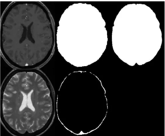
Figure 1:Example of brain mask extraction. Top line, from left to right: T1-w, result of bet and final result. Bottom line: T2-w and difference between both mask. On T1-w is difficult to precisely identify the external CSF space.
3.3 Skull Stripping
Skull stripping methods remove non-brain voxels from the image to simplify the following lesion seg-mentation. There are multiple methods described in the literature and several comparison studies were performed [12,6]. The skull stripping method from the FSL library is employed, called bet [13], used as previously described by Rex et al. [12] to improve its results.
This first algorithm employed is not perfect and usually leaves some non-brain voxels, mainly skull, optic nerve or veins. To improve the brain mask by removing the skull and the veins, we include information coming from T2-w and FLAIR images where veins and skull have low intensity. We use a 3-class model (in T2-w: CSF,brain tissues and skull/veins; and in FLAIR: CSF/skull/veins, brain tissues and lesions) in each sequence with a Expectation Maximization (EM) algorithm [4] to classify the voxels inside the first brain mask. Then only the voxels that have been classified in both sequences as the class with skull and veins are removed from the brain mask. An example can is shown in Figure1.
3.4 MS Lesions Segmentation
Our original method is called STREM (Spatio Temporal Robust Expectation Maximization)[1], and after introducing improvements to reduce the number of false positives, but also to apply STREM in datasets where only single time point MRI’s are available. MS lesion segmentation is performed with a three-step
3.4 MS Lesions Segmentation 4
process: 1. Robust estimation of Normal Appearing Brain Tissues (NABT) parameters, 2. Refinement of outliers detection and 3. Application of lesion rules.
Estimation of NABT parameters
NABT image intensities are modeled with a 3-class finite multivariate Gaussian mixture [16], where each class is associated to a different part of the brain: White Matter (WM), Grey Matter (GM) and CSF. All the MR sequences are used to create a multidimensional feature space in order to benefit from the specific inherent information of each sequence.
To calculate the NABT parameters we use a modified Expectation Maximization algorithm, called mEM, based on the Trimmed Likelihood (TL) Estimator [11]. It was shown to have a monotonous convergence, at least to a local maximum of TL, as the original Expectation Maximization (EM) algorithm. The idea is to use exclusively in our computation of TL the n − h voxels that are closer to the model and reject the h voxels more likely to be outliers.
T L= ∑n−hi=1 f(xν(i); Θ)
Where n is the total number of voxels, h the number of rejected voxels, xiis a vector with the intensities of
the m sequences of the voxel i, Θ the parameters of our 3-class model, f() the p.d.f. of the model and ν() is a permutation function which orders voxels so that:
f(xν(1); Θ) ≥ f (xν(2); Θ) ≥... ≥ f(xν(n); Θ)
The trimming parameter h is chosen arbitrarily with a high value, to ensure the rejection of all WML voxels from the computation of the NABT parameters. In our workflow the parameter h is set to the 10% of the pixels of the brain.
Refinement of outliers detection
In practice, the h rejected points actually contain some inliers that actually fit the NABT model reasonably well. Thus, to refine the outliers detection, we compute the Mahalanobis distance between each of the n voxels in the image and each NABT given the previously computed parameters. Considering that voxels intensities in each NABT follows a Gaussian law, these Mahalanobis distances follow a χ2 law with m d.o.f [1,5]. Each voxel in the image is defined as an outlier if the Mahalanobis distance for every class is greater than the threshold defined by the χ2 law, for a given p-value. In our workflow p-value is set to 0.4 to ensure all the lesion voxels will be taken into account although this means the existence of many false positives at this stage.
Application of lesion rules
Outliers found with the Mahalanobis distance may be originated from other tissue compartments than WML, basically due to partial volumes, vessels, registration errors, noise, etc. In order to discriminate between the WML and false positives, rules are defined with neurologists and neuroradiologists based on image intensities from the respective MR sequences and voxel connectivity.
Different intensity rules can be implemented for the different types of MS lesions [1]: black holes, Gadolinium-enhanced lesions and T2-w lesions. In this paper we focus in T2-w lesions that are, com-pared to the normal apperaring WM, hyperintense in T2-w and FLAIR, and isointense or hypointense (e.g. black holes) in T1-w. Hyperintense and hypointense voxels are defined by 3.0 × σW M±µW M, where σW M
and µW M are the standard deviation and the mean of the white matter respectively.
Voxel connectivity allows the use of neighboring rules instead of classifying each voxel independently. In this case, a minimal size of MS lesion is defined [2], so detected lesions that have a size smaller than 3 mm3 are discarded. We also remove detected lesions that are contiguous to brain border or not contiguous to WM tissue.
4
Results
Our workflow does not use any learning steps. Training datasets where not necessary for the final processing of the test images. Yet, we processed these datasets in order to verify that our segmentation workflow could handle these images. In those training datasets no numerical evaluation or optimization of parameters were performed.
4.1 Evaluation measures
Four different measures have been employed in the comparison of the automatic MS lesion segmentation with the expert manual segmentation. A normalization into a 0-100 range was performed [14].
• Volume Diff.: The volume difference captures the absolute percent volume difference to the expert rater segmentation.
• Avg. Dist.: The average distance captures the symmetric average surface distance to the expert rater segmentation.
• True Pos.: Number of lesions in the automatic lesion segmentation that overlaps with a lesion in the expert segmentation divided by the number of overall lesions in the expert segmentation.
• False Pos.: Number of lesions in the automatic lesion segmentation that do not overlap with any lesion in the manual segmentation divided by the number of overall lesions in the automatic segmentation. In addition a STAPLE algorithm [15] has been performed with the two expert segmentation and other auto-matic segmentation methods to compare their solutions.
4.2 Test images
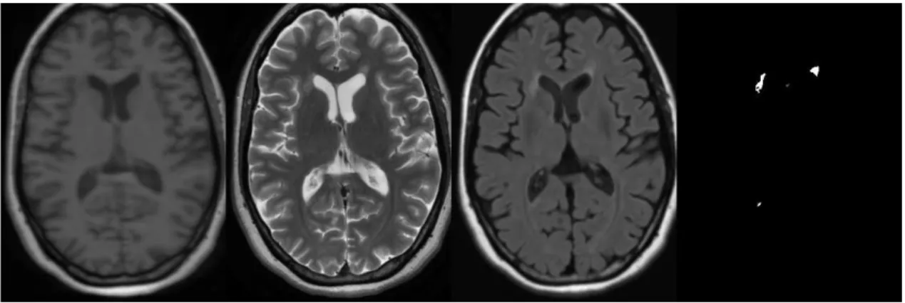
The described workflow does not include any manual or semi automatic steps. All the images were processed automatically with the same parameters. Table4shows the results for the test images. Average results show that we are far from the value of 90 associated with the inter rater variability in the normalized scale [14], but our results are independent of the center where MR acquisition was performed. An example of good lesion segmentation is given in Figure2
There are five datasets with scores under 70. CHB test1 Case15 was not processed because of a hu-man error and UNC test1 Case07 T1-w is likely to have been done after Gadolinium injection. In
6
Figure 2:Dataset CHB test1 Case08 : From left to right T1-w, T2-w, FLAIR and automatic segmentation results
Figure 3: Some artifacts (from left to right): CHB test1 06 T2-w and Flair, UNC test1 Case07 T1-w (we think Gadolinium-enhancing T1-w)
UNC test1 Case10, the low contrast between lesions in the FLAIR image could cause problems in the segmentation. We found that CHB FLAIR images usually have a drop in signal intensity in the superior part of the brain, see Figure 3, that the IIH correction method was not able to correct. In the case of CHB test1 Case06 and Case12 this intensity drop was large enough to alter our 3-class model giving low segmentation results. In those two datasets we also find strong movement artifacts but, as our method makes little use of the spatial information, these artifacts should be less critical in the performance as observed in the results of UNC test1 Case02.
5
Discussion
We have presented our fully automatic workflow for the segmentation of MS lesions. Our objective is to propose a method which is not based on training steps and can be used with different MR protocols or scanners yielding reproducible results. Looking at the available datasets for this validation study we strongly felt that the analysis of the results is not straight forward and there are several aspects that need to be discussed and improved for new future validations studies: definition of MRI lesion, quality of datasets and total lesion load of the patients.
Ground Truth UNC Rater CHB Rater STAPLE All Dataset Volume Diff. Avg. Dist. True Pos. False Pos. Volume Diff. Avg. Dist. True Pos. False Pos. Total Specificity Sensitivity PPV
[%] Score [mm] Score [%] Score [%] Score [%] Score [mm] Score [%] Score [%] Score
UNC test1 Case01 23.9 97 4.8 90 48.8 79 36.7 87 11.3 98 5.9 88 53.1 82 46.7 81 88 0.9892 0.5779 0.7154 UNC test1 Case02 32.4 95 4.2 91 52.9 82 43.1 83 91.1 87 4.4 91 36.4 72 13.8 100 88 0.9970 0.1357 0.8706 UNC test1 Case03 34.0 95 2.6 95 49.3 79 22.7 96 14.7 98 2.0 96 52.9 82 17.6 99 92 0.9912 0.7604 0.8260 UNC test1 Case04 37.1 95 3.5 93 50.0 80 46.2 82 2.4 100 2.0 96 59.3 85 56.4 75 88 0.9964 0.7203 0.9435 UNC test1 Case05 73.3 89 4.8 90 38.1 73 37.9 87 39.7 94 3.3 93 60.9 86 44.8 82 87 0.9971 0.2717 0.7924 UNC test1 Case06 41.5 94 11.9 75 37.9 73 75.0 64 161.4 76 20.4 58 62.5 87 86.1 57 73 0.9632 0.2049 0.2656 UNC test1 Case07 100.0 85 128.0 0 0.0 51 0.0 100 100.0 85 128.0 0 0.0 51 0.0 100 59 1.0000 0.0000 nan UNC test1 Case08 26.3 96 6.8 86 38.3 73 51.4 78 20.5 97 5.7 88 83.3 99 56.8 75 87 0.9882 0.5901 0.5895 UNC test1 Case09 23.9 97 18.9 61 33.3 70 96.9 51 7.4 99 26.7 45 100.0 100 96.9 51 72 0.9944 0.1331 0.3549 UNC test1 Case10 22.0 97 13.5 72 35.0 71 74.1 65 341.1 50 19.0 61 50.0 80 88.9 56 69 0.9971 0.6439 0.8902 CHB test1 Case01 68.1 90 5.5 89 26.7 67 25.9 94 54.5 92 3.2 93 51.6 81 40.7 85 86 0.9998 0.2566 0.9737 CHB test1 Case02 26.0 96 4.1 92 59.1 85 51.7 78 68.5 90 2.7 94 68.4 90 27.6 93 90 0.9986 0.3723 0.9302 CHB test1 Case03 75.3 89 4.3 91 50.0 80 12.5 100 88.1 87 9.4 81 40.0 74 25.0 94 87 1.0000 0.2420 1.0000 CHB test1 Case04 26.9 96 14.9 69 45.5 77 81.1 60 64.9 91 16.7 66 38.9 74 75.7 64 75 0.9888 0.0632 0.2282 CHB test1 Case05 56.9 92 13.5 72 40.7 75 69.4 67 91.8 87 9.8 80 56.5 84 58.3 74 79 0.9980 0.0451 0.5451 CHB test1 Case06 98.6 86 27.7 43 2.8 53 96.7 51 98.5 86 27.5 43 4.5 54 96.7 51 58 0.9990 0.0001 0.0108 CHB test1 Case07 83.0 88 12.6 74 21.7 64 80.6 61 89.7 87 6.7 86 28.9 68 68.1 68 74 0.9959 0.0480 0.4711 CHB test1 Case08 44.4 94 2.6 95 70.4 91 28.6 92 62.8 91 3.6 93 58.8 85 7.1 100 93 0.9999 0.4187 0.9956 CHB test1 Case09 71.4 90 6.4 87 22.8 64 17.8 99 75.9 89 5.5 89 19.1 62 13.3 100 85 0.9996 0.2229 0.9732 CHB test1 Case10 50.7 93 3.3 93 68.4 90 50.0 79 75.9 89 4.3 91 55.2 83 30.8 91 89 0.9994 0.1730 0.9359 CHB test1 Case11 67.0 90 10.0 79 22.7 64 64.7 70 89.3 87 11.2 77 31.0 69 55.9 76 77 0.9977 0.0806 0.6554 CHB test1 Case12 99.7 85 19.2 60 6.0 55 57.1 75 99.7 85 19.7 60 10.3 57 61.9 72 69 0.9998 0.0018 0.4072 CHB test1 Case13 77.4 89 4.7 90 50.0 80 16.7 99 86.1 87 17.1 65 28.6 68 0.0 100 85 1.0000 0.1864 1.0000 CHB test1 Case15 100.0 85 128.0 0 0.0 51 0.0 100 100.0 85 128.0 0 0.0 51 0.0 100 59 1.0000 0.0000 nan All Average 56.6 92 19.0 75 36.3 72 47.4 80 80.6 88 20.1 72 43.8 76 44.5 81 79 0.9954 0.2562 0.6988 All UNC 41.4 94 19.9 75 38.4 73 48.4 79 79.0 88 21.7 72 55.8 82 50.8 78 80 0.9914 0.4038 0.6942 All CHB 67.5 90 18.3 74 34.8 71 46.6 80 81.8 88 19.0 73 35.1 71 40.1 83 79 0.9983 0.1508 0.7020
Figure 4:Results for test images. For each measure the value is given in two different metric: real value in the left and a normalized value in the right.
5.1 Definition of MS lesion in MRI
Compared to the segmentation validation of other targets, MS lesion segmentation have an increased com-plexity. Today there is no consensus on a precise definition of MS lesion in MRI. This situation leads to a very high variability, in first place, in the detection. In second place, and once all the lesions have been detected, there is a still a high variability in contour of each lesion [9,17,7], as MS lesions not rarely lack a sharp border, but also because MS lesion size and border vary according to the MR sequence used [7].
5.2 Quality of datasets
Quality of MR acquisition is difficult to evaluate but image artifacts complicate futher image analysis and can decrease the detectability of the lesions. For example, UNC datasets were easier to segment as the have less artifacts. Mixing images with and without strong artifacts also complicates the analysis of the results as we have to distinguish between separate influences of MRI artifacts and robustness or accuracy of the segmentation methods. For validation purposes, the MR datasets may be divided in two groups according their acquisition: without and with strong artifacts. In addition, MR raw data should be available to allow the use of the whole segmentation workflow, as described in Section3.1.
5.3 Total lesion load of the MS patients
Accuracy of segmentation methods vary with the magnitude of lesion load or degree of atrophy, and should be taken into account when interpreting our results. In addition, the measures in the validation are very dependent on the total number of lesions: for example when there are only a few lesions missing one single
References 8
lesion will significantly drop True Positives while when there are many lesions True Positives will only decrease very little.
References
[1] L. S. A¨ıt-Ali, S. Prima, P. Hellier, B. Carsin, G. Edan, and C. Barillot. STREM: a robust multidimen-sional parametric method to segment MS lesions in MRI. Med Image Comput Comput Assist Interv Int Conf Med Image Comput Comput Assist Interv, 8(Pt 1):409–416, 2005.1,3.4,3.4,3.4
[2] F. Barkhof, M. Filippi, D. H. Miller, P. Scheltens, A. Campi, C. H. Polman, G. Comi, H. J. Ad`er, N. Losseff, and J. Valk. Comparison of MRI criteria at first presentation to predict conversion to clinically definite multiple sclerosis. Brain, 120 ( Pt 11):2059–2069, Nov 1997. 3.4
[3] P. Coupe, P. Yger, S. Prima, P. Hellier, C. Kervrann, and C. Barillot. An Optimized Blockwise Nonlocal Means Denoising Filter for 3-D Magnetic Resonance Images. Medical Imaging, IEEE Transactions on, 27(4):425–441, April 2008. 3.1
[4] A. P. Dempster, N. M. Laird, and D. B. Rubin. Maximum Likelihood from Incomplete Data via the EM Algorithm. Journal of the Royal Statistical Society, 39(1):1–38, 1977. 3.3
[5] G. Dugas-Phocion, M.A. Gonzalez, C. Lebrun, S. Chanalet, C. Bensa, G. Malandain, and N. Ayache. Hierarchical segmentation of multiple sclerosis lesions in multi-sequence MRI. In Biomedical Imag-ing: Macro to Nano, 2004. IEEE International Symposium on, volume 1, pages 157–160, April 2004.
3.4
[6] Christine Fennema-Notestine, I. Burak Ozyurt, Camellia P Clark, Shaunna Morris, Amanda Bischoff-Grethe, Mark W Bondi, Terry L Jernigan, Bruce Fischl, Florent Segonne, David W Shattuck, Richard M Leahy, David E Rex, Arthur W Toga, Kelly H Zou, and Gregory G Brown. Quantitative evaluation of automated skull-stripping methods applied to contemporary and legacy images: effects of diagnosis, bias correction, and slice location. Hum Brain Mapping, 27(2):99–113, Feb 2006. 3.3
[7] M. Filippi, M. Rovaris, M. P. Sormani, M. A. Horsfield, M. A. Rocca, R. Capra, F. Prandini, and G. Comi. Intraobserver and interobserver variability in measuring changes in lesion volume on serial brain MR images in multiple sclerosis. AJNR Am J Neuroradiol, 19(4):685–687, Apr 1998. 5.1
[8] Daniel Garc´ıa-Lorenzo, Sylvain Prima, J.-C. Ferr´e, L. Parkes, J.-Y. Gauvrit, N. Roberts, S.P. Morrissey, and C. Barillot. Quantitative evaluation of intensity inhomogeneity correction algorithms for Multiple Sclerosis. In Presented in CARS, 2008. 3.2
[9] J. Grimaud, M. Lai, J. Thorpe, P. Adeleine, L. Wang, G. J. Barker, D. L. Plummer, P. S. Tofts, W. I. McDonald, and D. H. Miller. Quantification of MRI lesion load in multiple sclerosis: a comparison of three computer-assisted techniques. Magn Reson Imaging, 14(5):495–505, 1996. 1,5.1
[10] J.-F. Mangin. Entropy minimization for automatic correction of intensity nonuniformity. In Mathe-matical Methods in Biomedical Image Analysis. IEEE Workshop on, pages 162–169, June 2000.3.2
[11] N. Neykov, P. Filzmoser, R. Dimova, and P. Neytchev. Robust fitting of mixtures using the trimmed likelihood estimator. Computational Statistics & Data Analysis, 52(1):299–308, September 2007. 3.4
[12] David E Rex, David W Shattuck, Roger P Woods, Katherine L Narr, Eileen Luders, Kelly Rehm, Sarah E Stolzner, David A Rottenberg, and Arthur W Toga. A meta-algorithm for brain extraction in MRI. Neuroimage, 23(2):625–637, Oct 2004. 3.3
[13] S. M. Smith. Fast robust automated brain extraction. Hum Brain Mapp, 17(3):143–155, November 2002. 3.3
[14] B. van Ginneken, T. Heimann, and M. Styner. 3D Segmentation in the Clinic: A Grand Challenge. In 3D Segmentation in the Clinic: A Grand Challenge. Miccai Workshop, pages 7–15, 2007. 4.1,4.2
[15] S.K. Warfield, K.H. Zou, and W.M. Wells. Simultaneous truth and performance level estimation (STA-PLE): an algorithm for the validation of image segmentation. Medical Imaging, IEEE Transactions on, 23(7):903–921, July 2004.4.1
[16] III Wells, W.M., W.E.L. Grimson, R. Kikinis, and F.A. Jolesz. Adaptive segmentation of MRI data. Medical Imaging, IEEE Transactions on, 15(4):429–442, Aug. 1996.3.4
[17] Alex P Zijdenbos, Reza Forghani, and Alan C Evans. Automatic ”pipeline” analysis of 3-D MRI data for clinical trials: application to multiple sclerosis. IEEE Trans Med Imaging, 21(10):1280–1291, Oct 2002. 5.1