Designing an orientation finding algorithm using human visual data

Designing An Orientation Finding Algorithm Using Human

Visual Data

by

Mojgan Monika Gorkani

Bachelor of Applied Science

Electrical Engineering

University of Toronto, 1991

Submitted to the Program in Media Arts and Sciences,

School of Architecture and Planning,

in partial fulfillment of the requirements for the degree of

Master of Science

at the

MASSACHUSETTS INSTITUTE OF TECHNOLOGY

June 1993

©

Massachusetts Institute of Technology 1993

Signature of Author..,.

Program in Media Arts and Sciences,

School of Architecture and Planning,

May 17, 1993

Certified by ...

...

...

Rosalind W. Picard

Assistant Professor

Perceptual Computing Group in the Media Lab

Thesis Supervisor

Accepted by ...

. J. r...

Stephen A. Benton

Chairperson

Departmental Committee on Graduate Students

MASSACHUSETTS INSTITUTE

OF TECHNOLOGY

[JUL 12 1993 Rotch

Designing An Orientation Finding Algorithm Using Human Visual Data

Mojgan Monika Gorkani

Submitted to the Program in Media Arts and Sciences, School of Architecture and Planning,

on May 17, 1993, in partial fulfillment of the requirements for the degree of

Master of Science

Abstract

An algorithm for detecting orientation in textures is developed and compared to results of humans detecting orientation in the same textures. The algorithm is based on the steerable filters of Freeman and Adelson (1991), orientation-selective filters derived from derivatives of Gaussians. The filters are applied over multiple scales and their outputs nonlinearly contrast normalized. The human data was collected from forty subjects who were asked to identify "the minimum number of dominant orientations" they perceived, and the "strength" with which they perceived each orientation. Test data consisted of 111 graylevel images of natural textures taken from the Brodatz album, a standard collection used in computer vision and image processing. Results on comparing the computer and humans' test data indicate they each chose at least one of the same dominant orientations on 95 of the natural textures. Of these textures, 74 were also in 100% agreement on the location of all the dominant orientations chosen by both human and computer. Individual cases which disagree are analyzed, and possible causes are discussed. Some apparent limitations in the current filter shapes and sizes are illustrated, as well as some effects possibly due to semantic influences and gestalt grouping.

Thesis Supervisor: Rosalind W. Picard Title: Assistant Professor

Designing An Orientation Finding Algorithm Based On Human

Visual Data

by

Mojgan M. Gorkani

Thesis for the degree of Master of Science at the

Massachusetts Institute of Technology

May 1993

T hesis R eader ...

William Freeman Research Scientist Mitsubishi Electric Research Laboratories, Inc.

T hesis R eader ... ... Josef Bigiin Research Associate Signal Processing Laboratory of the Swiss Federal Institute of Technology in Laussane

Contents

1 Introduction 2 Background

2.1 Estimating Orientation In the Fourier Domain . . . . 2.2 Filtering: Trade-offs And Desirable Properties . . . . 2.2.1 Number of Filters Required for Orientation Estimation . . . . 2.2.2 Quadrature Filters . . . . 2.2.3 Vectorial Representation of Filter Responses . . . . 2.2.4 Examples of Directional Filtering Methods Used for Orientation tion . . . . 2.3 Other Methods of Finding Orientations . . . . 3 Scale Problem

3.1 Choosing the Right Scales . . . . 3.1.1 Laplacian Pyramid . . . . 3.1.2 Steerable Pyramid . . . . 3.1.3 Adaptability in Scale . . . . 3.1.4 Other Multi-scale Analysis . . . . 4 Orientation Finding Algorithm

4.1 Orientation Histogram . . . . 4.1.1 Test Images . . . . 4.2 Analyzing the Orientation Histograms

4.2.1 Histogram Smoothing . . . . . 4.2.2 Finding the Prominent Peaks . 4.3 Dealing with Contrast . . . . 4.3.1 Contrast . . . . 4.3.2

4.3.3 4.3.4

Non-linear Transformation of th Contrast Enhancement of Image Contrast Normalization . . . .

. . . .

. . . .

. . . .

. . . .

. . . .

. . . .

. . . .

. . .

5.1 Human Visual Experiment . . . . 5.1.1 Subjects . . . . 5.1.2 Experimental Setup . . . .

5.1.3 Training Session . . . 73

5.1.4 Test Im ages . . . 76

5.1.5 Recording of the Human Visual Data . . . . 77

6 Comparison of Human and Computer Data 81 6.1 Organization of Human Visual Data . . . 82

6.2 Organization of Computer Data . . . 83

6.3 Comparison Between Orientations Picked by Humans and Estimated by Filters . 84 6.3.1 Results with the Different Thresholds Assigned to the Levels of the Steer-able Pyramid . . . 98

6.3.2 Results from Incorporating the Contrast Normalized Histogram . . . 106

6.3.3 Cases Where There was no Match between the Human and Computer Data115 7 Conclusion And Future Goals 120 7.1 Picking Better Thresholds . . . 121

7.2 Filters of Different Shapes . . . 121

7.3 Contrast Normalization . . . 121

7.4 Testing the Algorithm on Different Test Images . . . 122

A Teaser Images 123

Acknowledgments

First of all, I gratefully acknowledge the support of my advisor Roz Picard. She has always been encouraging and very patient with me (especially when I barge into her office and start talking non-stop about a problem). She is a great role model and someone that I have looked up to and will continue to do so.

Bill Freeman, my reader, has helped me tremendously with his steerable filter code. His help has been invaluable to me. Josef Bigiin was kind enough to be my reader and over long distance gave me great insight in the complicated task of finding orientations.

Oliver Yip helped me in developing and conducting the human visual test. Brad Horowitz offered his X-window expertise to develop the interface for the visual test. Ted Adelson gave me helpful comments about the human visual test and his four beautiful pictures which I have used in my introduction are greatly appreciated. I would like to thank Lee Campbell and Stephen Intille for their patient reading of my thesis and their helpful remarks. Irfan Essa, Stan Sclaroff and Ali Azarbayejani offered me their Latex and graphical tools expertise. Eero Simoncelli over the ethernet helped me with some theoretical questions. The Texture Heads : Fang Liu, Chris Perry, Kris Popat, Steve Mann, and Alex Sherstinsky gave me support and encouragement. Jeff Bilmes forced me to lift weights so that I would be strong enough to finish this thesis. John Wang helped me a lot with the Obvius software.

I would like to also thank all the subjects who took my visual test. Without their data, this thesis would not exist.

Thanks to my fellow officemates Sourabh Niyogi and George Chou for their stimulating conversations. And to the rest of Percom members including Bea Bailey, Laureen Fletcher and Judy Bornstein who one way or another helped me to finish this thesis. Thanks to Linda Peterson for being so understanding and giving me lots of encouragement.

Thanks to my patient and understanding roomate, Debbie Becker. Others who supported me along the way: Gilbert Chiang, Ilya Lyubomirsky, Eric Ly, Raj Gupta, Judy Chen, Wenjie Hu, Mary Beshai, Siegfried Fleischer, Grace Foster and many more.

Most importantly, I would like to thank my parents Mahmoud and Fakhry and my brothers Payman and Arman. My brother Arman has been my major source of support. It has been great living in the same city with him!

Chapter 1

Introduction

Imagine the future when vast amounts of image data such as movies, photo albums, journals and other visual collections will be available in databases and can be accessed online. Accessing this information fast and efficiently is a big challenge and offers a rich, new research area. BT (British Telecom) is funding a research project at the MIT Media Lab to develop tools which can search for a picture just like one can search for a keyword or a text description in a database. One major problem with image databases is that a short description attached to an image will not be sufficient for all queries. A more likely scenario is where a user shows a computer a pre-existing pattern and asks the computer to search for patterns similar to it. It is important to find visual features which describe the visual content in an image and can be used to judge the similarity between images.

One such visual feature is the dominant orientations of an image. For example, in Figure 1-1, the number of dominant orientations in each image is sufficient to discriminate the four textured images. There is psychophysical evidence that humans use orientation as a cue for discriminating textures [1][2][3]. Further, results from physiological experiments suggest the

existence of orientation selective mechanisms in the human visual system [4][5].

Extraction of orientation over a large scale can be used for rotating images to align before comparing them pixel by pixel - a process possibly performed by humans [6]. Shape and perspective information can also be obtained from relative orientation [7, 8].

As orientation is one of the most important features for human attention and for texture matching, it is important that algorithms which extract orientation be developed. One of the key difficulties in extracting orientation information is that it has to be gathered over multiple scales [9][10]. Also, orientation estimation is complicated by effects such as contrast, gestalt organization, and the semantic meaning associated with a pattern.

The research in this thesis focuses on the interaction of orientation estimation with scale and contrast. In particular, an algorithm is developed to find dominant orientations in tex-tured images combining the orientation information over four different scales and using contrast normalization. To evaluate the results of this algorithm in detecting dominant orientations, a human visual test was conducted. The human data was collected from forty subjects who were asked to identify "the minimum number of dominant orientations" they perceived, and the "strength" with which they perceived each orientation. Test data consisted of 111 gray level images of natural textures taken from the Brodatz album [11], a standard collection used in computer vision and image processing. The positions and the numbers of dominant orienta-tion found by the algorithm were compared with the human data. Some of the parameters in the algorithm were then varied to obtain better agreement between the human data and the algorithm.

Chapter 2 gives background information on orientation estimation techniques and compares several popular methods for finding orientations. Chapter 3 outlines problems in estimating

Bamboo Shoots Brick Wall

Funny Slots Impatiens

Figure 1-1: Four textured images (Printed with permission from E. H. Adelson).

orientations at different scales and reviews several multi-scale techniques for finding local ori-entations. Chapter 4 outlines the orientation finding algorithm used in this thesis for finding dominant orientations in textured images. Chapters 5 and 6 describe the human visual test and outline the comparison done between the human visual data and the computer data respectively. Conclusions and further work is discussed in Chapter 7.

Chapter

2

Background

An oriented pattern's Fourier transform tends to cluster along lines in the Fourier domain perpendicular to the orientations in the spatial domain. This clustering can be detected by summing energy in the appropriate region of the power spectrum and examining how the sum is affected by rotations. Most of the methods proposed for calculating main orientations are in essence finding the orientation along which this clustering occurs. In this chapter, I first talk about methods which operate directly in Fourier domain, then those based on filters in the spatial domain, and finally some other methods of finding local orientation.

2.1

Estimating Orientation In the Fourier Domain

Orientation can be estimated directly in the Fourier domain. Bajcsy [12] showed in her paper that directionality can be measured by calculating the histogram of the Fourier power along lines through the origin (see Figure 2-1). If F(wi, w2) is the Fourier transform of image I, then

Figure 2-1: The power spectrum is summed along each of these lines

P(wi, w2) from cartesian coordinates to P(r,

#)

r, Pr() is a one-dimensional function. She determined the main orientations by looking at the peaks of the histogram of directional power P(#) . P(#) is calculated for quantized values of

#,

#

(2.1)

P(#) = E pr(#)

r=1

where X is the window size. Bajcsy applied this method on several textures of size 32 ₂ x 32 where the quantized interval for

#

#

This method has several drawbacks. One problem involves the inherent difference between continuous and finite discrete Fourier transforms. Transforming from cartesian coordinates to

polar coordinates is tricky since it involves interpolation and the results are inaccurate near the origin. Bajcsy first high-pass filtered the images since the definition of angle is very coarse at low-frequency points due to the smaller number of samples available on the rectangular grid. Also low-frequency components are affected more by illumination changes than surface coloration [13]. However, false peaks were still found in the histogram of P(#) due to smooth changes in shading which are perceptually discounted by humans [12]. Bajcsy argued that more information about the scene (its illumination, continuity and context) is needed to remove this kind of slow change. If the oriented energy falls between two bins, the energy contribution from each bin will be small and will not be prominent in the histogram.

Chaudhuri, et. al. [14], extract orientation information by using sector filters on the Fourier transform of the image instead of summing the oriented power in the polar coordinates as Bajcsy. The filter rejects all the Fourier components outside the desired angle band. An ideal sector filter causes ringing and smearing artifacts. To overcome such affects, they multiplied the sector filter with a raised cosine window W1

(V):

W

(p)

_B

= 0 otherwise (2.2)

where V is defined as,

= arctan(!-) (2.3)

W

angle band and B = V2 - V1 is the chosen angular bandwidth. The value a is chosen to make sure that the window coefficients are not too low to miss the components near the two limits of the angle band.

Before applying the sector filter, the computed Fourier transform of the image is bandpass filtered which removes the very high and low frequency components to reduce the effects of aliasing, noise, illumination effects and having fewer sampling points near the origin. The cutoff frequency to remove the low frequency components depends on the nature of the input image. Depending upon the scale of a local structure, the cutoff frequency might suppress the contribution of the Fourier components of these structures. Chaudhuri, et. al. ran the sector filters with different p1 and V2 on images with structures at different orientations and inverse Fourier transformed the resulting filtered images. Ideally the inverse Fourier transformed images should contain the structures in the original image with orientations corresponding to the angular band of the filters. The distribution of orientations corresponding to the structures was found by counting the pixels of the binarized inverse Fourier transformed output images corresponding to the different angle bands. One problem they found was that for structures of finite width in the original image, the components in the frequency domain do not lie completely within the defined sector. As the thickness of the structures increases, there is an increased spreading of the Fourier components, leading to a reduced angular sensitivity. This results in poor contrast in the filtered components and certain artifacts.

2.2

Filtering: Trade-offs And Desirable Properties

Another way to detect the direction along which the clustering in the Fourier domain occurs is by filtering in the spatial domain. Filters in the spatial domain can be used to find local orientation information more easily than operating directly in the Fourier domain. Also there is psychophysical and physiological evidence that some of the primate receptive fields can be modeled by linear filters [15]. Filters can be chosen which select only the frequency components in a particular direction. The local orientation in an image can be found by running a set of directionally sensitive filters. If there is one main orientation then there will be a large response in the filters whose direction coincides most closely with the main orientation and the responses of all the other directional filters will be small. If a large fraction of filters give a comparable response then the neighborhood has structures covering all orientations.

The selection of the set of directional filters involves certain trade-offs. As mentioned before very low spatial frequency components should not be used for the orientation estimation since they are affected more strongly by illumination effects than surface coloration. Further, the definition of angle is very coarse at low-frequency points due to the smaller number of samples available on the rectangular grid [14]. On the other hand, high spatial frequencies are sensitive to noise and aliasing so they too are inappropriate for estimating orientation. To measure orien-tation some kind of bandpass filtering is preferable. Another trade-off occurs between angular and spatial resolution. If the filter is too orientation-specific then a large spatial neighborhood is needed to make reliable measurement of energy [13]. Conversely, if the filter responds over a wide range of orientations then it will be difficult to localize the orientation accurately. It makes sense then to choose filters which exhibit good local properties both in spatial and

fre-quency domains. Since Gaussians are optimally localized in space and frefre-quency, derivatives of Gaussians are often used as directional filters.

2.2.1

Number of Filters Required for Orientation Estimation

It seems initially that many filters at different orientations are needed to estimate the local orientation. It would be desirable to know how many filters are needed for an accurate mea-surement of orientation.

If a directional filter can be rotated to any orientation by a finite number of basis filters then the basis filters can be used to estimate the local orientation. If a two-dimensional filter in the spatial domain f(x, y) with polar representation f(r,

4)

4)=

and i =

S1i,

f

N

fa(r,4)=

n=-N

exp(-in6) as the coefficients needed to linearly combine them to synthesize filter g at any orientation [16]. The number of basis filters needed is determined by the number of positive and negative frequencies present in the polar frequency expression shown in (2.7). If all the an(r) are non-zero for all -N < n < N then 2N + 1 basis filters have to be used.

The basis filters can also be rotated versions of the filter. Freeman and Adelson in [16] derive the conditions needed to synthesize a filter

f

f:

K

f(x, y) = Zk;(O)fa (x, y). (2.8)

1=1

Filter

f

K

am(r) exp(imO) =

[k(6)am(r)

l=1

In (2.9) since -N < m < N, there will be 2N + 1 linear equations. The equations can be stated in the following format:

1 1 ... 1 ki(6)

exp(iO) exp(ia1) ... exp(iaK) k2(0)

where only the expressions for positive m are shown. To calculate the coefficients ki, however, expressions for positive and negative m have to be used. If am(r) = 0 for any m, then the corresponding (mth) row of the left hand side and of the matrix of the right hand side of (2.10) should be removed. Freeman and Adelson show that if T is the number of positive or negative frequencies where am(r) is non-zero for -N < m < N, then the required number of basis filters

K has to at least equal T. The T basis function orientations al must be chosen so that the

columns in the matrix in (2.10) are linearly independent. One way to ensure this is to choose these angles to be equally spaced between 0 and ir. An observation is that the interpolation functions k1(9) are independent of the values of the non-zero coefficients am(r); therefore, these

coefficients are not necessarily unique for a particular filter. This is true since the interpolation is only dependent on the angular tuning of the filters.

Freeman and Adelson also show in [16] that for filters of the form f(x, y) = W(r)PN(x, y),

where W(r) is an arbitrary windowing function and PN(x, y) is an Nth order polynomial in x and y whose coefficients may depend on r, a linear combination of 2N + 1 basis functions are sufficient to rotate filter

f

kj(9) for a set of separable basis functions W(r)RI(x)S(y) so that the rotated filter

fo

K

fo(x, y) = W(r) E k(6)Ri(x)S;(y) (2.11)

1=0

If a filter does not have a finite polar Fourier series representation then it can not be exactly steered by a finite number of basis filters. One solution is to approximate a kernel with an

adequate higher order polynomial multiplied by a radially symmetric function. To approximate the filter response from a limited number of basis filters, certain methods can be used to minimize the error in the synthesized filter as suggested by Perona in [17].

2.2.2

Quadrature Filters

Another requirement on the choice of the set of directional filters has to do with the phase dependency of the orientation estimate. If the directional filter is even about the axis of its main orientation then it will give a zero response along this axis when convolved with a signal which is odd along that axis. For example, a second derivative of a Gaussian filter outputs zeros along an edge oriented the same direction as the filter. Similarly, a directional filter which is odd about the axis of its main orientation such as the first derivative of a Gaussian will give

a zero response along this axis when convolved with a signal which is even along that axis. This means that even when the direction of the filter coincides with the local orientation of the image, the output of the filter can be zero. Two filters are said to be in quadrature if they have the same frequency response but differ in phase by 90*. In other words they are Hilbert transforms of each other [18]. Where one filter response shows zero crossings, the other one will show extremes. Let E(6) be the sum of the squared outputs of an oriented filter

f

E(6)

(ho

(2.12)

When the direction of filter

f

f

If we have a filter

f

f

H(wi, w2) = i sign[cos(<p -

4k)]F(wi,

where F(wi, w2) and H(wi, w2) are the Fourier transforms of

f

#k

the main direction of filter

f

The fact that a filter can be steered by a linear combination of basis filters does not mean that its Hilbert transform is also steerable. For example, the Hilbert transform of a second derivative of a Gaussian is not steerable by a finite number of basis filters. However, an approximation to the Hilbert transform can be found which is steerable. Freeman and Adelson in [16] formed an approximation to the Hilbert transform of a second derivative of a Gaussian by finding the least squares fit to a polynomial times a Gaussian which is steerable.

2.2.3

Vectorial Representation of Filter Responses

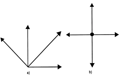
The responses of the directional filters can be represented as orientation vectors: the magnitude of the vector corresponds to the magnitude of the filter response, while the direction is given by the filter orientation doubled [19]. The local orientation can be computed by the vector addition of these orientation vectors. If there is a neighborhood containing structures in all directions, then the vector sum of the filter responses should vanish since there is no one dom-inant orientation. This does not happen if the direction of the orientation vectors corresponds

a)

b)

Figure 2-2: Computation of local orientation by vector addition of the four filter responses. Shown is an example where the neighborhood is isotropic with respect to orientation: all filter responses are equal. a) The angles of the vectors are equal to the filter directions. b) The orientations shown are double those in (a).

to the filter directions since the filters are usually equally spaced between 0 and 7r and there

is an equal contribution from each response. For example, in the case of the four directional filters, the sum will only vanish for this neighborhood if the angles of the orientation vectors

are double the filter orientations as shown in Figure 2-2. This makes sense since by doubling the angles of the filters, the orientation vectors will be uniformly distributed between 0 and 27r and will then cancel out if they have equal magnitudes.

In [19] Knutsson and Granland suggest directional filters fk which are polar-separable in the Fourier domain:

where < is defined in (2.3) and p is defined:

p 2 (2.15)

Fk(p, p) is the polar representation of the Fourier transform of fk, Fk(wi, w2). Vi(p) and V2(<p)

are functions of p and p respectively. V2(<p) for the fk are defined as:

V₂(p) = cos2P(W -

4k)

where ek is the main orientation of filter fk and the value p determines the angular resolution of the filter. If there are K directional filters, the main orientations k are equally distributed between 0 and yr where

4k

0

=k(60) exp(i27rk/K)V2(0) (2.17)

where fk is the vector representation of the output of fk. Note the factor 2 in the complex exponential results from doubling the filter orientation since the direction of the vector is double the filter orientation.

vector whose angle is double the local orientation:

K-1 K 2p

E k(6) = exp(i200) (2.18)

k=O _p

P+

This is true provided that p > 0 and K > p + 1.

Note that the condition for (2.18) to be true is very similar to the criterion for the number of basis filters needed to synthesize a filter at any orientation. Recall that the number of basis filters needed corresponds to the number of frequencies for which the an(r) coefficients of the Fourier polar series representation are non-zero as shown in Section 2.2.1. The polar component V2(<p) can be represented as a Fourier polar series representation and there will be p+2 non-zero

Fourier polar coefficients.

2.2.4

Examples of Directional Filtering Methods Used for Orientation

Esti-mation

A number of methods have been suggested to measure the local orientations in textures using directional filters. The choice of the directional filter is difficult because it is hard to satisfy all the requirements discussed in the previous section. Also there is a desire to choose filters which yield frequency and orientation bandwidths which are in reasonable agreement with the physiological and psychophysical estimates of the early human visual processes. The following examples are representative of some of the methods currently used and do not cover all the possible ways of measuring orientation. It should be mentioned beforehand that the local orientation 00 estimated in the methods below is perpendicular to the perceived orientation.

Kass and Witkin's method [13]

Kass and Witkin find the main directionalities in a texture by examining the energy in the output of an orientation-selective linear filter fk.. Their choice of the orientation-selective filter is:

w0f(x, y) = (cos 0, sin 0) - Vq

= Cs O~_4 ep- (z2 + Y2) _4 ep- (z2 + y2)

= cos 6(z(oejexp( 2 (72 P(x 2

2oal 2a2

-- (2 2+ Y2) ( 2-x 2

+

+

+ )-) 4 P(X2 ) (2.19)

2a, 2o,2

where a1 and 02 are the variances of isotropic Gaussian filters. This filter is bandpass and its frequency tuning is identical to the first derivative of a Gaussian. The filter

fk,

V(6) = Mg*(fkw*I)2

V(O) = mg * (cos(6)Cx + sin(O)Cy)2 (2.20)

where mg(x, y) is Gaussian weighting function, I is the image, and Cx and Cy are the outputs of the image convolved with the basis filters. This oriented energy is very similar to E(6) shown in (2.12) except that the Hilbert transform of the oriented filter was not calculated by Witkin and Kass. The weighting function mg is used to average the results in order to reduce the noise in the calculation of the energy. Averaging the squared output of the directional filter response also makes the energy V(6) independent of the input phase. However, using the quadrature

method discussed in Section 2.2.2 provides a better spatial resolution since averaging with mg will blur the oriented energy V(6).

If (2.20) is expanded, V(O) will be in terms of cos 26 and sin 26; therefore, it will be periodic with a period of 7r and will have two extrema 7r apart. Also, since V(6) is in terms of cos(26) and sin(26), the orientation found from analyzing V(6) will be double the desired local orientation 6. The orientation 6, is found by calculating the peak of V(6) in the following way:

t f V(6) sin(G)dO 0 farcta V() cos(O)dO 2 arctan( "*Cj/G )

_(2.21)

If complex variable Pkw is defined to be

Pkw = (CX +iCY) 2 _(2.22)

then angle 6 and the measure of reliability of the orientation (also frequently called "coher-ence") Xkw, can be expressed in terms of Pkw:

200 = arg(Pkw * mg) (2.23)

| Pkw *mflg

Xkw = - (2.24)

(IPkwI|

As can be seen, Pk. is a combination of the basis filter outputs and can be regarded as an orientation vector where 200 would be the direction of an average of these vectors in a local neighborhood. The measure of reliability for the orientation calculated for pixel position (x, y)

is reflected in how well the Pk. vectors are lined up in a local region around position (x, y).

Bigiin and Granlund's method [20]

Even though this method initially does not appear to use directional filtering, its implementation in the spatial domain results in using directional filters. Bigiin and Granlund define an image to be "linear symmetric" if it is made up of a set of parallel lines. The Fourier transform of a linear symmetric image is shown to be exactly concentrated to a line through the origin. Of course, most real-life textures are not linear symmetric. However, if they have a strong orientation their Fourier transforms should be spread about a line through the origin. Bigin and Granlund find the main orientation in the least-squares sense by fitting a line through the Fourier transform of the texture. The optimally fitted line in LSE sense represents the axis of least inertia of the Fourier transform and can be found by finding the smallest eigenvalue of the 2 x 2 inertia matrix J,

fE

f

w|F(w,

w

)|

_dE

2

-fE

f

w

IF(w1,

W

)|

dE

(2.25)

-fJE

f

wiw

|F(w1, w

)j

dE

f

w2IF(wi,

w

)I

2

_dE

2

where

F(wi,

dE

independent of the input Fourier phase.

J can be calculated in the spatial domain for a local neighborhood and its approximate discrete representation consists of:

u

= _{) 2* m}

47r

= 1

I)

J2-41r2(6 bX m

1 6I16I

J12 = J21 = - * mg (2.26)

41r2 bx by y

where g, 6 are the discrete Gaussian derivatives of the image I , my is a Gaussian filter and

Jmn is the (m,n)th component of J.

The optimal line 9 is the orthonormal eigenvector corresponding to the smallest eigenvalue of J called A,. The other eigenvalue A1 corresponds to the line perpendicular to 9. The main direction represented by angle 0,, is calculated to be

tan(260 ) = 2J12 (2.27)

J1 1 - J2 2

where Jmn is the (m,n)th component of J. Two measures of the reliability of the estimation of

the orientation, Xbgl and Xbg2, are calculated

Xbgl = A1 0 )c (2.28)

A\1

+

Ao

Xbg2 = A₁ - Ao (2.29)

where A1 and AO are the two eigenvalues for J (2 x 2) and c is a constant used to control the

dynamic range of Xbgl so that it is less dependent on the contrast of the image. Bigiin and Granland do not discuss how c should be chosen for different images. The values c = 1 and c = 6 were used to illustrate how the value of c affects the coherence measure.

optimal fitted line. This occurs if the energy in the Fourier domain is distributed in such way that there are many lines which give the same least square error. (See Figure 2-2(b)). In this case the values for Xbg1 and Xbg2 will be close to zero since the difference between the eigenvalues

is close to zero. The least eigenvalue A, will be zero and will have a multiplicity of one if and only if image I is linear symmetric. In this case Xbgl will ideally be equal to 1 and Xbg2 will be equal to the value of the biggest eigenvalue, A1. If the value for A1 is large then Xbg2 will

be large. A high Xbg2 indicates that the orientation found is reliable which makes sense since A, must be very small compared to A,. If both eigenvalues are zero then the image is constant (has no main orientations). Combining (2.27), (2.28), (2.26) and using the variable Pg defined as:

P g i 2 (2.30)

x

by

the values for 0,, and Xbgl and Xbg2 can be expressed in the following way:

20, = arg(Pbg

*

Xbg1 = Pbg *

mg

(IPbgI* mg)

Xbg2 = 12 JPbg * mgI. (2.33)

For each point (x, y) in image I, the local orientation 0, and the measures of reliability Xbg1 and Xbg2 can be calculated.

Rao and Schunck's Method [21]

Rao and Schnunk used a directional filter, f,, which is a first derivative of a Gaussian. The first derivative of a Gaussian is a steerable filter:

f

where g and g 0" are the first derivative of Gaussians oriented at 00 and 900. Since

f,,

00*_g 0

1

-6x

I*g '

_--

_(2.35)

1 by

where b and b are discrete Gaussian derivatives of I.

The local orientation 0, is then calculated in the following way:

200 = arg(Pbg * mb) (2.36)

where Pbg is defined in (2.30) and mb is a box filter. The orientation measure is analogous to Bigiin and Granland's method (2.31) except that a box filter is used instead of a Gaussian filter. The same result as (2.36) can be obtained by minimizing the oriented energy E(9) with respect to 0 in equation 2.12 with

fe

ff,

Granland's smoothing with the Gaussian filter mg.

The measure of the reliability or coherence measure of the orientation estimated for position

(xO, yO) Xra is:

E;(i,j)EL

xr,9 -- ,: R~x YO) (i,j)E L G(zi, yi) (.7

where R(xz, yo) is the magnitude of the gradient at position (xo, yo) , L is the local region where

this measurement is calculated and 00(xi, y;) is the orientation found at position (xi, y;). The

coherence Xr, is a measure of how well the gradient vectors line up with respect to the gradient vector at position (xo, yo). The R(xO, yo) component is used as a weight to make sure that X,, is high at points where there is high visual contrast. It is not clear how the size of the local region L is chosen.

Freeman and Adelson's method [16]

Freeman and Adelson use the second derivative of a Gaussian to estimate the local orientation. The second derivative of a Gaussian, 92 is then defined as:

g2(x, y) = 0.92132(2x

2

- 1) exp(-(x2 + y2)) (2.38)

and is normalized so that the square of its integral equals to one over all space. The corre-sponding representation is:

92(r, #) = 0.92132r2 exp(-r

2_{) cos(24) + (r}2

where r and

4

a, = 0.92132(r2 - 1) exp(-r 2₎

a2 = a- 2 = 0.46066r2exp(-r 2) . (2.40)

Since there are three non-zero coefficients a.(r), three basis filters are needed to steer

92

three x-y separable filters whose linear combination can steer 92 to any orientation. The x-y

separable basis filters for 92 will be denoted 920, 921 and 922:

920 = 0.9213(2x2 _ 1) exp(-(x2 + Y2

))

921 = 1.843xyexp(-(X2

+

922 = 0.9213(2y2 _{_ 1) exp(-(x}2 _{+ y}2_{)) (2.41)}

As mentioned in Section 2.2.2, the Hilbert transform of 92 is not steerable. Freeman and Adelson approximate this Hilbert transform with a least squares fit to a polynomial times a Gaussian which is steerable. They found an approximation, h2, using a 3rd order, odd parity

polynomial:

h2 = (-2.205x

+

The x-y separable basis filters for h2 will be denoted

h

,

.

To find the main orientation in a local neighborhood, the oriented energy described in (2.12) will be calculated for image I. Since go and he can be expressed as a linear combination of their basis functions, E(6) can be expressed in the following way:

E(6) = (g*I)2

+(I

2 3 =

((E

+

((Z

(E

+

(Z

(2.43)

where kgI 0 < I < 2 are the interpolation functions to steer 2 and khl 0 < n < 3 are the interpolation functions to steer h2. As can be seen in (2.43) to calculate E(6), image I just has

to be convolved with the basis filters for 92 and h2. The interpolation functions for a particular

9 can then be used to give the oriented energy. For 92 and h2, the interpolation functions are

[16]:

kgl

=

(-

)l

2

cos2-

(0)

sinl(6),

0

<

1 < 2

(2.44)

3

khn

= (-1)"

cos

_-"(6)

_sin"(6),

₀

<

n

<

_3.

_(2.45)

n/

Freeman and Adelson in [16] show that the interpolation functions are products of cosines and sines. Because of the squaring operation in (2.43), E(6) can then be simplified to a Fourier series in angle, where only even frequencies are present:

E(O) = C1 + C2 cos(20) + C3 sin(26) + higher order terms (2.46)

where C1, C2 and C3 are a combination of the basis filter outputs.

The dominant orientation 0, can be approximated by using the lowest frequency terms and by maximizing E(6) with respect to 0. Freeman and Adelson show that the solution for 0, will be:

0 - arg(C3, C2) (2.47)

The strength of the orientation estimation S is defined as:

S=

The approximation stated in (2.47) is exact if there is only one dominant orientation locally. The dominant orientation measure and its strength S is measured at each pixel position (x, y). If there is more than one dominant orientation locally, then the approximation is not correct and other methods have to be used to find the orientations.

Discussion of the Four Methods

The calculation of the local orientation 0, in Rao and Schunck's method is identical to Bigiin and Granlund's method except that Rao and Schunck use a box filter for local averaging and Bigiin and Granland use a Gaussian filter. It is not clear which filter is more appropriate for making the orientation estimation independent of input phase and reducing the noise. The two-dimensional box filter is a poor low-pass filter and its transfer function is not isotropic, i.e., it depends, for a given frequency, on the direction of the frequency. Also, since its Fourier transform is a sinc function, the attenuation in frequency domain tends to oscillate instead

of increasing monotonically with the frequency [22]. The orientation estimation of Kass and Witkin's is identical to Bigiin and Granlund's method except that the directional filters are different. The angular tuning of the two methods, however, are identical.

The "coherence" measure of Bigiin and Granlund Xbgl when c = 1 is expressed the same as Kass and Witkin's coherence measure Xk. Rao and Schunck's coherence measure Xbg1 is different from Kass and Witkin's and Bigiin and Granlund's. Rao and Schunck show for one textured image that their coherence measure gives a better result than Kass and Witkin's measure. One of the reasons for the difference in the results may be that Rao and Schunck use the magnitude of the gradient, R(xz, yo), to emphasize high visual contrast. The inclusion of the R(xz, yo) component may enhance the fine details in the image more than the other two coherence measures. On the other hand, a high contrast structure with no dominant orientation might have a false coherence measure due the R(xz, yo) component.

The strength measure in (2.48) used in Freeman and Adelson's method is the absolute strength of an estimated orientation as determined by the energy output of the directional filters. The coherence measures of the other three methods, on the other hand, give an indication of how dominant an orientation is in a local region. If there are many different orientations of equal absolute strengths in a local neighborhood, then the coherence measure for any of these orientations will be very small even though their absolute strength could have been large. Choosing the right size for the local region used in the coherence measure is not clearly explained in any of the methods. Because the coherence measures are ratios of the outputs of the filters, two orientations of differing contrasts can have the same coherence measures unless the absolute strength of orientation is also incorporated as is done in Section 2.2.4 by Rao and Schunck.

estimation independent of input phase. The other three methods average the energy output of the directional filters. This averaging is effective for making the orientation estimation independent of input phase; however the spatial resolution in the orientation estimation is lowered because of blurring from averaging.

All of the methods use steerable filters. The first derivative of a Gaussian is used in both Bigiin and Granlund's method and Rao and Schunck's method. The orientation tuning of Kass and Witkin's filter is identical to the first derivative of a Gaussian. Freeman and Adelson use a second derivative of a Gaussian. The second derivative of a Gaussian has a finer orientation tuning than the first derivative of Gaussian; however, it needs three basis filters instead of two to steer. There is psychophysical and physiological evidence supporting the use for both of these derivatives and higher order Gaussian derivatives to model cortical receptive fields [15].

2.3

Other Methods of Finding Orientations

Andersson in [23] uses a non-steerable set of filters with a much finer orientation tuning than the filters in the methods discussed above. If there is only one dominant orientation then there is not a big difference between Andersson's method and the methods discussed above although Andersson does not prove that that the number of filters he used (between 18 to 24 filters) is sufficient to estimate all orientations uniformly. If there are multiple orientations, such as lines crossing at different orientations, then near the point of intersection the filters in the methods discussed above may give false orientation estimates because of their broad angular tuning. Andersson's filters on the other hand will give a more accurate result since they have a narrower angular tuning. Higher order derivatives of Gaussians can also be used to detect finer

angular spacing because of their narrow angular tuning. These derivatives are also steerable; however, the higher the order of the derivative, the greater the number of basis filters needed to steer it.

The local orientation can also be estimated by finding the direction of the principle axis of image I in a local region using moments [24]. Bigiin and du Buf in [25] show that the second orders complex moments of the local Fourier power of image I can be used to find local orientation. They also show that higher order of complex moments can be used to detect N-folded symmetries. The latter may also have important applications for image comparison; the focus in the thesis however will be on detection of perceptually dominant orientations, symmetric or not.

Chapter 3

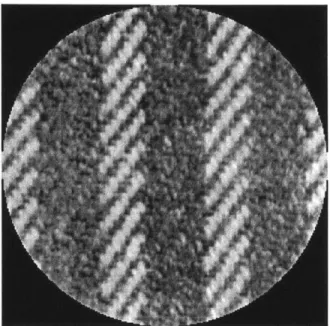
Scale Problem

In an image there can be textures at different scales like Figure 3-1 (Brodatz image D11). Measuring texture features at the right scales is still a big problem in texture analysis. Sev-eral multiresolution or multichannel methods for texture analysis have been developed such as Gabor decomposition [26] [25] and Tree-structured wavelets [27]. Orientation detection is also dependent on scale. Several methods can be used to measure orientation at different scales. These methods will be reviewed and compared in this section.

3.1

Choosing the Right Scales

One strategy for resolving the scale problem is to measure the dominant orientations over different scales. The two big questions with this strategy are:

1. How many scales should be evaluated and what should they be?

Figure 3-1: Image with orientations at different scales.

Due to the computational costs required to generate filters over a continuum of scales and storage of the filtered images, usually, a discrete, small set of scales is employed.

3.1.1

Laplacian Pyramid

A computationally efficient way to obtain a discrete, small set of scales is by computing a pyramid. The Gaussian pyramid consists of a series of images obtained by repeatedly smoothing and subsampling an image [28]. The pyramid allows large scales to be brought into the range of a local neighborhood. Overall, the computation of this pyramid requires only four thirds of the operations necessary for the first level [28].

Running a Gaussian pyramid on textured images might not be appropriate since some textures are quasi-periodic signals whose dominant frequency channels are located in the middle frequency range [27]. _{For these textured images, a bandpass decomposition appears more}

appropriate. The Laplacian pyramid is an effective scheme for this kind of decomposition. It can be obtained by subtracting the smoothed image from the unsmoothed image on each level of a Gaussian pyramid [28]. Applying the Laplacian pyramid on an image results in frequency channels whose scale doubles from level to level of the pyramid, while the center frequency of the passband is reduced by an octave. The Laplacian pyramid is a complete representation of an image in a sense that one can perfectly reconstruct the original image given the coefficients in the pyramid. Completeness is an important property since it guarantees that no information is lost, i.e., if two images are different then their representations will be different [29].

Bigiin in [30] uses the Laplacian pyramid for multiscale analysis of orientations. His orienta-tion finding algorithm involves calculating Pbg described in (2.30) at each level of the pyramid. However, applying the first derivatives of Gaussians as required for the calculation of Pbg causes the coefficients of the Laplacian pyramid to change. The coefficients can no longer be used to perfectly reconstruct the original image. This will cause some Fourier components to be em-phasized more than others and the orientation estimation will no longer be independent of the frequency content of the estimated orientation.

Also, if the texture appears in a scale which coincides exactly with one of the bandpass frequency channels, i.e., located near the maximum response of the channel then its orientation information will be obtained in the corresponding level of the pyramid. However, if the scale does not coincide near the maximum response of the channel then the frequency components associated with this scale will be attenuated and the texture will appear in low contrast in the resultant pyramid image. As can be seen, the problem of contrast and scale are not independent.

3.1.2

Steerable Pyramid

In [31], a multiscale structure called the steerable pyramid is constructed allowing orientation estimation at different scales. The steerable pyramid corresponds to a series of images obtained by repeatedly bandpass filtering, low-pass filtering and subsampling the image. Figure 3-2 shows a block diagram of two stages of the steerable pyramid. L0(wi, w2) and L1(w1,W2) are

low-pass kernels and B(wi,W2) is a bandpass kernel. The input image is convolved with the

bandpass kernel B(wi,W2) and a low-pass kernel L1(wi,w2). Running the steerable pyramid on

an image results in a spectral decomposition shown in Figure 3-3. The overall response of the pyramid is flat in the frequency domain. The original image can be reconstructed by adding the overall response of the pyramid with a high-pass residue image.

The band-pass filter B(wi,W2) in the steerable pyramid is constrained by the flat low-pass

response of the pyramid. A symmetric 15-tap bandpass filter was used by Simoncelli et. al. [31] to approximate this bandpass filter. To use this bandpass filter for estimating orientations, an angular frequency response A(9) = i cos3(0) is multiplied by the radial response. The result is a directional filter. A(9) can be expressed as :

A(6) = i - cos(30) + - cos(O) . (3.1)

(4 4

In Fourier polar representation (3.1) corresponds to four non-zero polar coefficients an(r); therefore, four basis filters are needed to steer the bandpass filter to any direction. Figure 3.1.2 shows mesh plots of the desired angular symmetric frequency response and the imaginary com-ponent of the frequency responses of the basis filter set. The angular tuning of this directional filter is finer than the directional filters discussed in Chapter 2 and is identical to a third

Figure 3-2: Block diagram of two stages of the steerable pyramid (adopted from [31]).

(02

Figure 3-3: Illustration of the spectral decomposition performed by the steerable pyramid (adopted from [31]).

derivative of a Gaussian. At each level, these four basis filters are applied to the image. When the basis filters are applied again at each level, the filtered version (original image minus the high-pass residue) can be recovered.

As discussed in Chapter 2, to make the orientation estimation independent of the input phase, the Hilbert transform of the directional filter is found. An approximate Hilbert transform is found which is steerable with 5 basis filters. For multiscale orientation estimation, the oriented energy as described by (2.12) is maximized at each level of the pyramid. The image size over which the orientation is estimated decreases with the number of levels because of the subsampling. The estimated orientation and its strength, (2.47) and (2.48) can be found for each pixel (x, y) for each level. For the steerable pyramid, C2 and C3 in (2.48) are combinations

of the outputs of the basis filters for the directional filter and its Hilbert transform. The number of levels for the pyramid is dependent on the size of the image and the size of the directional filter kernel.

Because the bandpass filters have to satisfy the flat low-pass response of the pyramid, the orientation estimation will be independent of the frequency content of the estimated orientation. However, as in the case of the Laplacian pyramid, if a texture appears in a scale which does not correspond to the maximal response of the filters associated with the pyramid then the frequency components corresponding with that scale will be attenuated and the output of the directional filter will be small. It may be difficult to detect the orientation existing in that scale.

(a)

(b) _(c)

(d) _(e)

Figure 3-4: Frequency domain response plots: a) Desired angular symmetric two-dimensional frequency response. (b)-(e) Imaginary component of the frequency responses of the resulting steerable basis set. The functions shown here are the same as in [31].

3.1.3

Adaptability in Scale

Another way to estimate the orientation at the right scales is to have filters which are adaptable in orientation and scale: a minimum number of filters can be used to interpolate the local scale and orientation. The dominant orientation can then be found by first maximizing the filters over scale and then over orientation. The requirements for a filter to be adaptable over scale can be easily illustrated for a filter

f

F(p, p) = Vi(p)V2(o) (3.2)

where F(p, W) is the polar coordinate representation of the Fourier transform of

f

as a linear combination of basis filters:

K

V(p) = E Sj(p)kj(p) (3.3)

i=1

where S are the basis filters. Observe that (3.3) looks very similar to (2.7) where filter

f

and exists for all (positive) frequencies; hence, it can not have a Fourier series representation. It is then not possible to generate a continuum of scales spanning the whole positive line [17]. This may not be necessary since the range of scales of interest is never the entire real line. An interval of scales: