HAL Id: hal-02290142
https://hal.sorbonne-universite.fr/hal-02290142
Submitted on 17 Sep 2019
HAL is a multi-disciplinary open access
archive for the deposit and dissemination of
sci-entific research documents, whether they are
pub-lished or not. The documents may come from
teaching and research institutions in France or
abroad, or from public or private research centers.
L’archive ouverte pluridisciplinaire HAL, est
destinée au dépôt et à la diffusion de documents
scientifiques de niveau recherche, publiés ou non,
émanant des établissements d’enseignement et de
recherche français ou étrangers, des laboratoires
publics ou privés.
physical and biological properties
Yannick Huot, David Antoine, Chloé Daudon
To cite this version:
Yannick Huot, David Antoine, Chloé Daudon. Partitioning the Indian Ocean based on surface fields
of physical and biological properties. Deep Sea Research Part II: Topical Studies in Oceanography,
Elsevier, 2019, 166, pp.75-89. �10.1016/j.dsr2.2019.04.002�. �hal-02290142�
Contents lists available atScienceDirect
Deep-Sea Research Part II
journal homepage:www.elsevier.com/locate/dsr2
Partitioning the Indian Ocean based on surface
fields of physical and
biological properties
Yannick Huot
a,∗, David Antoine
b,c, Chloe Daudon
daDépartement de Géomatique appliquée, Université de Sherbrooke, Sherbrooke, Québec, J1C 0A5, Canada bRemote Sensing and Satellite Research Group, Curtin University, Perth, Western Australia, 6845, Australia cSorbonne Université, CNRS, Laboratoire d'Océanographie de Villefranche, LOV, F-06230, Villefranche sur mer, France dInstitut Physique du Globe de Paris, Université Paris-Diderot, USPC, 75205, Paris Cedex 13, France
A B S T R A C T
Comprehensively sampling the ocean in situ remains a challenge, even in the current era of rapid technological development. In less than a decade, the deployment of thousands of autonomous profiling floats increased the number of ocean temperature profiles by an order of magnitude compared to ship-based sampling in the past. But expendablefloats cannot sample all the physical and biogeochemical regimes in the global ocean. A promising avenue that could guide in situ sampling is to partition oceans based on selected properties in order to identify“homogeneous” areas. This approach greatly reduces the number of measurements needed to represent the state of the ocean. However, homogeneous areas can be partitioned in many ways: depending on whether a single or several properties are considered; and on whether the definition of boundaries is left to expert knowledge or derived from objective analysis techniques. Here, we use a clustering method to map and partition many surface variables, and we further examine how this partitioning is affected by various ways of averaging or normalizing the input data. We performed this study using 15 different surface fields of physical and biological properties derived from satellite remote sensing observations and from global model outputs at a monthly resolution. The area of study is the Indian Ocean - one of the least-sampled oceans - which is the focus of a global research effort under the auspices of the second International Indian Ocean Expedition (IIOE-2). We show a strong effect of the average absolute values of the data, which can be removed to better examine the phenology of the properties. However, normalization is not mandatory; the technique selected should depend on the scientific questions at hand. Our clusters did generally did not match closely the regions identified by Longhurst in his seminal work on ocean provinces.
1. Introduction
Covering more than 70% of the Earth's surface, the upper ocean is vast and spatially heterogeneous. Biogeophysical heterogeneity is a characteristic of the ocean appreciated by many: “snowbirds” head south to enjoy beaches and warm waters, while fishermen choose frontal regions to increase their catches. Oceanographers, too, have been aware for centuries of ocean spatial variability, which they have described and quantified. By carefully collecting data and contouring, global ocean atlases have described many physical and chemical properties (e.g.,Locarnini et al., 2013). Satellite images of water tem-perature and surface phytoplankton abundance arefinally showing the true complexity of this spatial heterogeneity at the global scale. Ad-vances in numerical modeling and computing power now allow many of these large-scale and mesoscale patterns to be reproduced. These patterns can be verified with satellite data, and the models can be va-lidated below the upper layer using observations from autonomous robots.
Our observational and modeling capacities have grown tre-mendously in recent years. Nevertheless, satellites provide estimates of
only a limited number of variables for the very upper layer of the ocean (sometimes tens of meters but generally much less); robots can only carry a limited suite of sensors, especially when it comes to chemistry and biology; and model outputs will always be limited to their para-meterization, which must stem from in situ or laboratory measure-ments. To understand many of the finer processes occurring in the ocean and how they respond to environmental changes, it remains necessary for oceanographers to spend time at sea in order to collect in situ measurements. Some process studies can be carried out almost anywhere, but studies aiming to describe and understand how processes vary spatially on large scales, as well as temporally, require statistically representative sampling. Covering large areas with afine spatial and temporal grid is impossible using ships. One solution to this problem is to partition the ocean into “homogeneous” areas based on selected physical, biological and chemical properties. Sampling a few points in space and time in such a“homogeneous” area would then allow the resulting values to represent the whole region.
In the context of the second International Indian Ocean Expedition (IIOE-2, Hood et al., 2016), we were interested in reassessing ap-proaches to partition the Indian Ocean basin in order to provide basic
https://doi.org/10.1016/j.dsr2.2019.04.002
Received 2 December 2017; Received in revised form 18 December 2018; Accepted 1 April 2019
∗Corresponding author.
E-mail addresses:yannick.huot@usherbrooke.ca(Y. Huot),david.antoine@curtin.edu.au(D. Antoine).
Available online 05 April 2019
0967-0645/ © 2019 The Authors. Published by Elsevier Ltd. This is an open access article under the CC BY-NC-ND license (http://creativecommons.org/licenses/BY-NC-ND/4.0/).
partitioning for cruise planning and also to map key oceanographic features.
Many studies have proposed partitioning the ocean using different approaches and input variables (see review ofDowell et al., 2009). We will not review them but will refer to appropriate references when discussing our results. Many studies use satellite input (and sometimes other geospatial data) together with a clustering algorithm to identify homogeneous regions. In most cases (but see,Lévy et al., 2007) when the Indian Ocean has been included in such an exercise, it has not been specifically targeted and has instead been included as part of a global analysis. Since it covers about one-fifth of the ocean surface (and less if the Southern Ocean below∼40˚S is excluded), it has a low weight in statistical clustering approaches applied at a global scale, so that unique features of this basin may be missed, such as the very strong impact of the South Asian monsoon.
A key body of work in understanding the ecological provinces of the Indian Ocean is a series of papers and books by Longhurst and co-au-thors (Longhurst, 2007; Longhurst et al., 1995) in which expert knowledge was used to identify biomes and provinces in the global ocean. These studies are particularly important because they are not simply based on an automated statistical approach, but rather use a priori knowledge of oceanic processes. As such, they provide a basis for comparing and understanding the results arising from statistical ap-proaches for partitioning the ocean.
Among the myriad approaches for partitioning ocean waters, a distinction must be made between“static” and “dynamic” partitioning. In the static approach, most often used for the description of biomes on land, the province boundaries do not change over time and the pro-vinces remain statically bounded. In dynamic approaches, the bound-aries are allowed to change on varying timescales (limited by the fre-quency of the input data used to delineate the regions). Beyond a changing climate, which affects both land and ocean, there is a clear argument for the presence of dynamic provinces in the pelagic ocean where currents transport water masses and their associated organisms and physicochemical properties. In addition, the turnover times of planktonic organisms dominating the pelagic ocean are much shorter than those dominating land ecosystems such that changes in the cli-matic conditions of a region can be rapidly reflected in its biota (e.g.,
Kintisch, 2015). Therefore, dynamic approaches are important for identifying regions where water column properties are similar over short times scales and where rapid changes in biota or ecophysiological parameters can occur (such as biomass-specific photosynthetic rates, which can respond within hours to days to changes in forcing Platt et al., 1991). For longer climatic-scale events and slower changing properties (e.g., regions with or without spring blooms), static pro-vinces are more relevant as they reflect regions that share common physical forcings and similar biota over longer time scales. This is conceptually closer to the partitioning of biomes and ecological pro-vinces on land where changing seasons do not alter the partitioning. Static partitioning is the focus of our study.
We have two main objectives for this study. Thefirst is to provide a small biophysical atlas of the Indian Ocean derived from state-of-the-art satellite remote sensing data and modeling results that shows homo-geneous regions with respect to different variables. While space limits the size and the number of the maps in this paper, the supplementary materials provide access to full size images as well as additional maps (additional variables and months depending on thefigures) not pre-sented herein. The second objective is to examine how different ways of using the same data (e.g., using either climatologies or time series, and using either unmodified or normalized data) provide different in-formation about the ocean. We have not examined the impact of dif-ferent clustering approaches (e.g., fuzzy, density-based, decision trees). Rather we have focused on a single method (k-means; see later) for all partitioning.
We briefly discuss some general oceanographic interpretations of the clusters and their temporal variability, but a full interpretation is beyond the scope of this paper as the interpretation of the partitions must largely be made within the context of specific questions. We also provide supporting information that could be useful for further analyses of the spatio-temporal distributions.
2. Materials and methods
2.1. Data used
We used data from four different sources: the Moderate Resolution
Table 1
Datasets used and symbols.
Source
Variable (algorithm; units; symbol/abbreviation used)
Timespan
MODIS AQUA sensor (Monthly climatology) Jul. 2002–Jun. 2014
Chlorophyll concentration (OC3M; mg m−3; Chl)
CDOM Index (Morel and Gentili, 2009; unitless; CDOM index)
Daily photosynthetically available radiation (PAR) (Frouin et al., 2003; mol m−2day−1, EPAR)
Sea surface temperature (Minnett et al., 2004;˚C; SST) Detrital and gilvin absorption (QAA; m−1; adg)
Optical backscattering coefficient of particles (QAA, m−1, b bp)
AQUARIUS sensor
Wind speed (Fore et al., 2014; m s−1; N/A) Sept. 2011–Sept. 2015
Salinity (Meissner et al., 2014; PSS; N/A) Aug. 2011–May 2015
HYCOM (daily data, averaged to monthly climatologies) Sept. 2008–Apr. 2014
Mixed layer depth (see text; mld, expt_90.6 to expt_91.0; m; zMLD)
Surface current speed (HYCOM; expt_90.6 to expt_91.0; m s−1; not abbreviated)
NCEP DOE AMIP-II reanalysis (daily means, averaged to monthly climatologies) Jan. 2000–Dec. 2014 Total cloud cover (Kanamitsu et al., 2002; %; N/A)
Wind speed (Kanamitsu et al., 2002; m s−1; N/A)
Downward solar radiationflux (Kanamitsu et al., 2002; W m−2; N/A) Precipitation rate (Kanamitsu et al., 2002; kg m−2s−1; N/A)
Derived quantities (Calculated from the monthly climatological means) Jul. 2002–Jun. 2014 Integrated mixed-layer chlorophyll concentration (see eq.(1); mg m−2; Chlint)
Euphotic zone depth (see eq.(2); m; zeu)
Ratio of the mixed layer depth to the euphotic zone depth (see eq.(4); unitless FeuMLD) Average irradiance in the mixed layer (see eq.(5); mol m−2day−1; E¯PAR)
Biological rate ratio (see eq.(6); Unitless; FT 23.9)
Imaging Spectroradiometer (MODIS) AQUA sensor; the AQUARIUS sensor; the Hybrid Coordinate Ocean Model (HYCOM); and the National Center for Environmental Prediction (NCEP-DOE) reanalysis (seeTable 1for a complete list of variables, abbreviations and symbols). As afirst step, we standardized the time and spatial resolution of each of these datasets. This was achieved by using monthly climatologies for all variables, which provided good spatial coverage of the Indian Ocean for all variables. Because the estimates of chlorophyll concentration (Chl) are key to clustering ecological regions, we used the MODIS AQUA level 3, 9-km standard mapped data as a reference and all other datasets were spatially interpolated to the grid center location of this dataset (2D-linear interpolation). Regions below 42˚S were excluded from our analysis because of the low solar zenith angle in winter and unavailability of MODIS data. For the AQUARIUS dataset, we used extrapolation tofill coastal points.
Five pre-processing methods, resulting in 5 data types were applied, in which the monthly climatological time series were:
1 averaged into an annual climatology (1 point for each pixel); 2 used to derive their standard deviation (1 point for each pixel), 3 used unmodified (12 points for each pixel);
4‘normalized’ at each pixel by the yearly mean of the pixel (12 points for each pixel);
5‘standardized’ by subtracting the annual mean and then dividing by the annual standard deviation (12 points for each pixel).
Each of these data types highlights different properties of the data (seeTable 2). Since the data spanned about two orders of magnitude for chlorophyll concentration, adg and bbp (see Table 1 and definition
below), the data were always logarithmically transformed (base 10) first, unless they were normalized or standardized, in which case no further transformation was applied. Since the annual variance is gen-erally proportional to the average annual concentration, this avoids regions with much higher values from dominating the selection of centroids during clustering.
We used the MODIS and AQUARIUS monthly climatologies dis-tributed by NASA (http://oceancolor.gsfc.nasa.gov/cgi/l3). For the other variables, the monthly climatologies were generally not available and were calculated from the daily data. Table 1provides the time period over which the data was collected to compute the monthly cli-matologies.
Beyond the most common variables, we also included optical vari-ables that are less often examined. We briefly describe them here. The adgis the absorption coefficient of gilvin and detrital substances, often
referred to as‘yellow substance’; it gives coastal waters brownish colors but is present in small concentrations everywhere in the ocean (Nelson and Siegel, 2013). In the open ocean, it arises mostly from the decay of organisms, while in coastal waters it is largely driven by land runoff. Photolysis removes this colored material in surface waters. The CDOM index is a measure of the amount of detrital substance relative to the expected concentration for a region given the amount of phyto-plankton. It reflects a departure in the ‘detrital material to living ma-terial’ ratio. It is centered on 1, values above 1 imply that there is greater detrital material to living material than expected (it can reflect
an increasing source or a decreasing sink for detrital material). The bbp
is the optical backscattering coefficient of particles in suspension. It reflects the concentration of particles in the water.
2.2. Clustering
We used the k-means algorithm with the Manhattan distance me-trics for the clustering analysis. The results using the Manhattan dis-tance were found to be less affected by outliers and provided cluster centroids that did not show large spikes. Such spikes were present when using standard Euclidean distance metrics. The clusters were computed using MATLAB 2017a, using the built-in algorithm in the statistics and machine learning toolbox (in this toolbox, the Manhattan distance is referred to as“city block”). To reduce the risk of finding local minima during clustering, the clusters were computed 10 times with different initial cluster positions, and the clusters with the lowest sum of the point to centroid distances were kept.
The k-means method requires a number of clusters to be specified a priori. Many objective methods have been developed to identify the optimal number of clusters to use. The“NBclust” R statistical software toolbox (Charrad et al., 2014) tests 30 different published indexes to
find the optimal number of clusters (the authors recommend using the number of clusters that arises the most often in the 30 indexes). The number of clusters selected by the different methods varied greatly (from 2 to 13) when we used the chlorophyll concentration as a test variable, with 2 being the most frequently selected number of clusters. Given that 2 was an unrealistically low number and that there is no consensus in the literature on the appropriate metric to estimate the optimal number of clusters, we turned to a more subjective approach where we initially set the number of clusters to 10, which is the number of Longhurst provinces in the Indian Ocean. We then evaluated the impact on the results of changing the values around this number and finally settled on eight clusters.
When clustering time series, the cluster centroids were obtained using all available pixels that had 12 months of data available. A large region in the northern Arabian Sea had no measurements in the AQUA Level 3 archive for July and August in the ocean color dataset. In order to cluster this region for the MODIS data (and the data derived from them), we assigned the pixels with missing data to the class of the centroid derived in the rest of the Indian Ocean over 12 months from which we removed the missing months before assigning the class.
2.3. Derived quantities
We also calculated some derived quantities from the measured and modeled variables obtained from MODIS and HYCOM, as follows.
The integrated chlorophyll over the mixed layer (Chlint, mg m−2)
was computed as: =
Chlint Chl z· MLD. (1)
where Chl (mg m−3) is the MODIS-estimated chlorophyll concentration, and zMLD(m) is the mixed-layer depth from HYCOM, computed as the
depth where the temperature increases by 0.2 °C from its surface value. The depth of the euphotic zone,zeu (m), which is defined as the
Table 2
Data type and property of the data that has the strongest influence on the clustering output.
Data type Properties of the data emphasized
Annual climatology (from averaging the monthly climatology data) Average value of the variable Standard deviation“climatology” (from calculating the standard
deviation of the monthly climatology data)
Variability of the variable
The time series unmodified Yearly average value has an overwhelming impact on the clustering output, with a secondary effect of the amplitude of the annual variation. Timing of the variation has little impact.
Time series divided by the annual mean The annual cycle amplitude and shape (timing) of the annual cycle. Time series standardized The shape (timing) of the annual cycle.
depth where net photosynthesis is null, has been approximated as the depth where irradiance is equal to the average compensation irradiance Ec= 0.17 mol m−2day−1fromTable 2inMarra et al. (2014),
⎜ ⎟ = − ⎛ ⎝ ⎞ ⎠ z K E 1 ln 0.17 . eu dPAR PAR (2)
This parameterization of the euphotic zone depth accounts for both the amount of incident irradiance and its attenuation in the water column, instead of only considering the latter when using the 1% light level (Banse, 2004). It ignores some spectral effects and the small
im-pact of sea-surface reflection.
In Eq.(2), EPAR(mol m−2day−1) is the average daily downward
photosynthetically available radiation (PAR, the integrated downward irradiance, Ed, from 400 to 700 nm) at the surface obtained from the
MODIS algorithm (Frouin et al., 2003), and KdPAR is the diffuse
at-tenuation coefficient for PAR and is calculated according to Morel et al. (Morel and Maritorena 2001version derived over thefirst two optical depths for Ed(490)):
= + −
KdPAR 0.0665 0.874Kd(490) 0.00121/Kd(490). (3) where K (490)d is the diffuse attenuation coefficient for Ed(490).
The ratio of the mixed layer to the euphotic zone depth, FeuMLD
(unitless), is then calculated as: =
FeuMLD z /z .
MLD eu (4)
The average PAR irradiance in the mixed layer (E¯PAR, mol m−2
day−1) is computed as:
∫
= − E z E e dz ¯PAR 1 . MLD z PAR k z 0 MLD dPAR (5) Wefinally computed the ratio of the biological rates relative to the mean temperature in the Indian Ocean. Using the monthly climatology, we computed the average annual temperature of the Indian Ocean (over the latitudes used here), which we found equal to 23.9 °C. By assuming a temperature sensitivity (Q10) of 2 (Raven and Geider, 1988; value consistent with the temperature sensitivity of photosynthetic and maximum growth rates in algae; seeEppley, 1972), we computed the ratio of the biological rates at a given temperature relative to this average temperature as= −
FT 2T .
23.9 (MODIS 23.9)/10 (6)
Biological rates do not respond to temperature exactly in this manner because acclimation and adaptation allow phytoplankton to change their cellular quotas in response to temperature changes (cel-lular photoacclimation to low temperature is similar to acclimation to high light,Maxwell et al., 1994). Nevertheless, Eq.(6)reflects a coarse
measure of temperature on phytoplankton physiology.
3. Results and discussion
3.1. Physical forcing
The physical forcing at the surface of the ocean influences many biological processes. Such dependencies are well known from previous studies, and we highlight here some key characteristics of the physical fields (Figs. 1–4; seeTable 2for the source of the data) that help to interpret the cluster distributions.
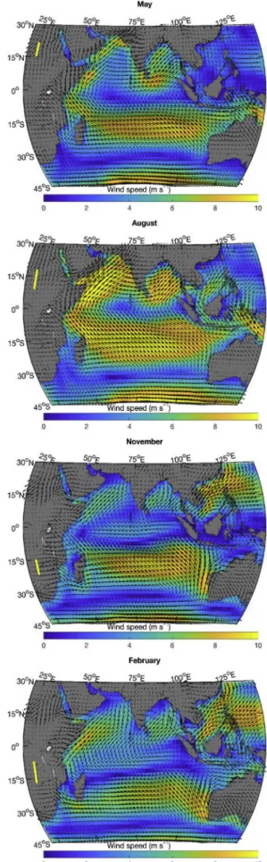
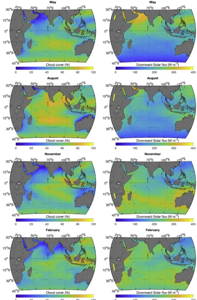
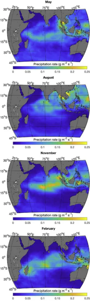
The Indian Ocean is strongly influenced by the South Asian mon-soon, which leads to strong southwest trade winds during the boreal summer (Fig. 1, see the August panel), peaking in July when the in-tertropical convergence zone (ITCZ) is located above the Asian con-tinent. This brings heavy cloud cover (Fig. 2) over the northern Indian Ocean. As is the case most of the year, the cloud cover at that time is higher in the eastern part of the ocean (Fig. 2). This leads to an east–west asymmetry in the downward solar flux (Fig. 2) and
Fig. 1. Average monthly wind speeds and direction (NCEP DOE reanalysis). The yellow line along the 25° meridian shows the sun declination angles spanned during that month. (For interpretation of the references to color in thisfigure legend, the reader is referred to the Web version of this article.)
Fig. 2. Average monthly cloud cover (left) and downward solarflux (right). The yellow line along the 25° meridian shows the sun declination angles spanned during that month. (For interpretation of the references to color in thisfigure legend, the reader is referred to the Web version of this article.)
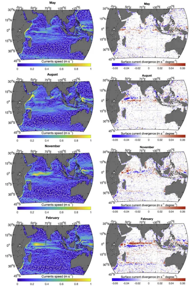
precipitation (Fig. 3) is heavier in the east. The southwest monsoon winds lead to anticyclonic circulation north of the equator (Fig. 4); currents at the equatorflow westward, while north of the equator in the Arabian Sea and the Bay of Bengal the circulation is generally eastward (see,Fieux, 2010;Tomczak and Godfrey, 2005). An upwelling zone also forms along the Somali coast (Fig. 4, strongly positive surface diver-gence in August) and the east coast of India in the presence of the strong southwest monsoon winds. East of the Maldives, a structured diver-gence zone is observed along the equator and a converdiver-gence zone is observed around 5˚N. During this period (seeFig. 1, August panel), winds are blowing from the continent to the ocean along the northwest coast of Australia leading to particularly clear skies, high irradiance and low precipitation.
In February, the northeast monsoon winds (actually the northeast trade winds) reach their maximum velocities in the northern Indian Ocean (Fig. 1). The anticyclonicflow in the Arabian Sea has essentially disappeared, and the anticyclonic circulation in the Bay of Bengal is much reduced; both regions have much less structured flow. The equatorial current has shifted northward (now referred to as the North Equatorial Current) and strengthened. The upwelling along the Somali coast has been replaced by a downwelling zone (Fig. 4). At this time of year, the divergence along the equator is strongest (see also,Koné et al., 2009), while a convergence zone is observed south of the equator (Fig. 4). Dry air from Asia brings nearly cloudless weather to the northern Indian Ocean (Fig. 2). The band of precipitation (Fig. 3) and low wind (Fig. 1) has followed the ITCZ that is now straddling the 15˚S parallel (slightly more south in the west and more north in the east), bringing a large band of clouds (extending north of the ITCZ) and lower surface irradiance. Along the northwest coast of Australia, the winds have also reversed bringing clouds and rain to the region.
Except in northwest Australia, the regions at latitudes south of 15˚S follow seasonal changes in solar irradiance and cloud cover; however, the wind patterns do not reverse. The subtropical ridge region is clearly seen as a band of low winds and cloud cover (∼30˚S to 35˚S) and re-mains at a more or less constant position all year. The zone just north of the subtropical ridge around 27˚S shows an interesting feature between December and March (February is shown inFigs. 1–4), where a zone of oceanic divergence (at∼27˚S) is adjacent to a zone of convergence at about 32˚S (Fig. 4). This corresponds roughly to the zone where large episodic blooms of phytoplankton (Longhurst, 2001) have been ob-served in late summer in some years.
Transitions between the monsoon periods occur around May and November as the ITCZ moves near the equator and monsoon winds are much reduced. At these times of year, the equatorial current reverses direction andflows east. In November, a broad divergence zone is ob-served east of Somalia, while the equator east of the Maldives becomes a convergence zone. A weak divergence zone is observed along the west coast of Sumatra throughout the year.
3.2. Clustering yearly climatological measurements
3.2.1. Average
Thefirst clustering analysis was based on the yearly average of in-dividual properties. This partitioning was carried out with a k-means algorithm, and regions with similar absolute values were grouped to-gether (Fig. 5).
Similar to the observations above on the physical forcings, this approach clearly highlights a strong east-west gradient in several phy-sical variables north of approximately 15˚S. This is particularly striking in the salinity distribution that shows lower salinity in the region with the most precipitation (Fig. 3), cloudiness (Fig. 2) and lowest solarflux (Fig. 2). The surface waters are warmer and less saline than in western regions. These general trends obtained from satellite data match well the maps of the World Ocean Atlas (Locarnini et al., 2013) that were computed from in situ data. South of the Arabian Sea and Bay of Bengal, the chlorophyll concentration is also lower in the east than in the west.
Fig. 4. Average monthly current (left column) and surface divergence (right; upwelling in red and downwelling in blue) from the HYCOM model. Current arrows are not proportional to the current speed and show only the current direction. (For interpretation of the references to color in thisfigure legend, the reader is referred to the Web version of this article.)
An even stronger north-south dichotomy is present with a boundary at around 10˚S to 15˚S for variables like wind speed, SST, ΔSST, and chlorophyll. The southern region is characterized by stronger winds, generally lower EPAR, deeper zMLD, and much larger temperature
var-iations. Note that the FT
23.9 clusters expectedly resemble those in SST
and, as such, we will use this ratio because it is a more direct measure of the impact of temperature on biological rates (it is also conveniently scaled and dimensionless). Between 15˚S and 30˚S, much lower phyto-plankton abundances are found in the subtropical gyre region, which lead to deeper zeu reaching around 180 m in the clearest part of the
gyre. By comparing the maps of zeu, chlorophyll concentration and
EPAR, it is clear that the attenuation coefficient of PAR irradiance, here
parameterized as a function of Kd(490) (and functionally similar to
Chl), has an overwhelming influence on zeucompared to EPAR; the use of
a percentage of incident surface irradiance is thus not a bad approx-imation - at least over the latitudes examined here– as a first estimate
of the depth of the euphotic zone (but seeBanse, 2004for the limita-tions of this approach). Similarly, adgroughly follows Chl and therefore
the same north-south gradient. The north-south gradient is also ob-served in the day-night difference in surface temperature. Because this difference is largely driven by wind speed (and solar irradiance), with lighter winds and higher irradiance increasing the daily difference (Gentemann et al., 2003), the distributions largely reflect the wind
speed patterns superimposed on a north-south gradient. Regions north of 10˚S have a much stronger daytime stratification than more southern regions.
Some of the derived variables seem to transcend these north-south and east-west gradients. Such is the case of E¯PARand FeuMLD. Both result
from the combination of zMLD, EPARand KdPAR(driven mostly by
phy-toplankton absorption/chlorophyll concentration). The average irra-diance in the mixed layer is strongly affected by the attenuation coef-ficient and also reflects the complex interplay of the attenuation, the
Fig. 5. Clustering of the annual climatology (average) for the 15 variables identified. Color bars show the range of values within each cluster, except for the upper and lower clusters, which extend (uppermost and lowermost value of highest and lowest cluster respectively) to 2 standard deviations from the cluster centroid value. The white lines correspond to the province boundaries identified byLonghurst (2007). (For interpretation of the references to color in thisfigure legend, the reader is referred to the Web version of this article.)
incident irradiance and mixing depth. The depth of the mixed layer also has a strong influence onChlintin that layer. The shallower mixed layer
north of∼15˚S leads to almost uniformChlint(∼3 mg m−2) for much of
the open ocean between 15˚N and 30˚S. The bbpdoes not appear to
covary with any other variable. It shows surprisingly low values in the eastern Arabian Sea and in the Bay of Bengal, while in the gyre, unlike in other gyres (e.g.,Brewin et al., 2012;Huot et al., 2008), it does not seem to follow the changes in chlorophyll. The high backscattering values south of∼40˚S have been associated with the presence of coc-colithophores (“the great calcite belt”Balch et al., 2011), but the pre-sence of higher winds (inducing bubble formation) and higher Chl concentration (causing an increased concentration of particles of all sizes) could also contribute to this elevated backscattering.
This analysis provides clusters for chlorophyll that are similar to those in the analysis byHardman-Mountford et al. (2008), who used principal component analysis to objectively map oceanic regions. In our study, the partitioning based on average annual chlorophyll is the most similar to the partitioning proposed byOliver and Irwin, (2008), who used normalized water leaving radiance (nLw) at 443 and 551 nm as
well as SST to identify their regions. This highlights the strong impact of Chl on the Oliver and Irwin provinces, through its impact on nLw.
For our next analyses, we decided to drop the CDOM index and the day-night temperature differences because they were noisier in the data types that were examined next; we also dropped SST, which is re-dundant with FT
23.9(they are provided in thesupplementary materials).
3.2.2. Standard deviation
The variance or its derived standard deviation is also informative as it allows grouping regions according to the amount of yearly variation within the regions (Fig. 6); this allows identifying stable vs variable regions. For parameters such as the chlorophyll concentration, zMLDand
to some extent adg, the maps based on the standard deviation show
spatial distributions that are similar to the maps based on average va-lues (Fig. 5). Most other variables show very different patterns. As an example, the incident EPARvariable does not show the east-west
gra-dient seen in the average maps but shows a mostly latitudinal gragra-dient as expected from solar insolation changing with season. Similarly, variability in the SST (presented as FT
23.9) shows very distinct patterns
from those in the annual climatology maps. In particular, a strong east-west gradient is present at all latitudes with the eastern side of the gyre showing much less variability in FT
23.9.
The eastern equatorial region extending to about 10˚S and 5˚N shows particularly low variability in most variables (except for salinity and bbp). This feature is likely due to low wind speed and high water
temperature that lead to a stable and well-stratified ocean with little variability. The shallowest zMLD according to HYCOM in the Indian
Ocean are, however, found in the western region between 0 and 15˚S (Fig. 5).
The sharp boundary that marks the North Subtropical Front (NSTF) between∼33˚S and 37˚S (depending on longitude) in the euphotic zone depth variable is a striking feature of these maps. South of the front, the increased irradiance in summer is almost exactly compensated by the increased attenuation due to chlorophyll (and associated material) such that the depth of the euphotic zone remains stable. This feature would not be observed if using the 1%-light level as the depth of the euphotic zone since it would only be determined by light attenuation. This fea-ture also highlights the slight inaccuracy in the boundary of Longhurst's ocean provinces in this region. Reygondeau (Reygondeau et al., 2013
theirFig. 3) also observed this departure in the static version of their classification of the Indian Ocean.
3.3. Clustering time series
Instead of using one measurement to capture the mean or variability of the time series, clustering the complete time series allows each time point, in this case monthly observations, to vary independently. It
allows separating different annual patterns even if the annual mean or standard deviation in two regions are similar.
3.3.1. Un-normalized time series
The simplest approach to use the times series is without any mod-ification (apart from the log transform for variables that span several orders of magnitude). In this case, the absolute value of the times series has a large impact on the clustering analysis, and most of the variables (Fig. 7) have distributions that resemble the average maps (Fig. 5). With the addition of the temporal aspect, the separation of the different clusters tends, however, to be stronger. Two variables that show dif-ferent clustering patterns when using the time series are EPARand E¯PAR.
In the (simpler to describe) case of EPAR, the presence of very different
annual cycles (more or less affected by the monsoon and/or cloudiness) leads to a very distinct distribution of clusters. North of 15˚S in the time series clustering, there is a clear north-south clustering with the northern regions showing a stronger effect of the monsoon (cycles that show two minima per year). The north-south clusters are further se-parated in an east-west fashion with the eastern portion showing higher irradiances due to lower cloudiness. In a similar, but less distinct, fashion from the average maps, the FT
23.9variable also separates along an
east-west gradient. A region in the northern Bay of Bengal and in the Arabian Sea shows the distinct bimodal monsoon features.
The annual cycles of bbpshow that the minimum and very low
va-lues in the Bay of Bengal occur from January to February when the mixed-layer depth is deepest and monthly wind speeds are nearly at the lowest values measured in the whole Indian Ocean. The highest values of bbpin the southern portion of the study area, previously referred to as
‘the great calcite belt’ (Balch et al., 2011), also occur around that time of year.
The annual cycles of the mixed-layer depth show that the east-west difference in the depth occurs mostly during the austral winter months, when the mixed layer is deeper in the eastern region by about 20 m. This feature does not seem to be reflected in the remotely measured fields (Chl, bbp, adg, salinity).
A strong north-south separation occurs in the adgvariable around
the equator (this was also observed but less obviously inFig. 5). This strong feature is not seen in any other variable. Values north of the equator tend to show more seasonality and/or higher values, which are perhaps linked to the relative proximity to the continent.
3.3.2. Time series normalized by the annual mean
The relative changes in the variables can be examined by dividing the time series by its annual average (Fig. 8). This approach removes the effect of the average value of a property and the spatial distribution of the clusters becomes very different from those obtained by using the time series without normalization. As described inTable 2, normalizing by the mean emphasizes at the same time the amplitude (related to the standard deviation examined in section 3.2.2) and the shape of the annual cycle. For time series of variables that show little variability compared to the mean, such normalization by the mean leads to clus-ters that have little meaning. This is certainly the case for salinity (apart perhaps in the northern Bay of Bengal), and the clusters appear to be very heterogeneous and without links to oceanographic or atmospheric patterns.
For some variables, there is an interesting added value in the re-lative changes that helps to understand the processes. For example, EPAR
highlights very clearly the increasing annual variability in the irra-diance with increasing latitude, with only a slight effect of clouds su-perimposed in the equatorial region. In all regions, irradiance values match their yearly average twice a year (i.e., a value of 1 inFig. 8) near the equinoxes. The E¯PARhas similar patterns to EPAR, though with more
variability in the latitudinal patterns as it is influenced by zMLD.
Simi-larly, the SST, here presented as FT
23.9, shows a mostly north-south
gradient. The effect of the monsoon in the north region is emphasized relative to the un-normalized time series. South of 10˚S, there is a clear
east-west separation where the western region has lower variability in the FT
23.9(pale blue cluster; similar to what was observed inFig. 6). In a
similar fashion to the EPARcentroids reaching their mean annual value
at the equinox, FT
23.9values reach their annual mean twice a year in
mid-November and at the beginning of March. The heating and cooling cycle is controlled by the net heat flux; this “crossing” of the annual average is later in the year than the incident irradiance.
The chlorophyll and zeucluster in a similar fashion. Compared to
previous clusters (e.g.Fig. 7), the spatial distributions are more scat-tered, with more mixing between the clusters as a large part of the variance was removed by the normalization. In addition to showing similar regions to those previously identified (e.g., Arabian Sea, east coast of Africa, stable region in the eastern equatorial Indian Ocean in
Fig. 7), it highlights new regions and some regions in different ways. In particular, it highlights a region that includes the Mozambique Channel and southwest of Madagascar, which is characterized by an increase in chlorophyll concentrations from December to June, which is very dis-tinct from all other clusters (and influenced by the episodic blooms described in section3.1). South of 30˚S, there is also a very strong
la-titudinal (but varying with longitude) clustering. Apart from the cluster southwest of Madagascar, the gyre region between 15˚S and 30˚S clusters in three groups with differences in the timing and amplitude of the annual chlorophyll cycle. The eastern region (green cluster in the chlorophyll panel) shows less variability in a manner that is consistent
with the F23.9T clusters.
This clustering approach is very similar to the approach followed by
D'Ortenzio and d'Alcalà, 2009 in the Mediterranean Sea; they used weekly instead of monthly averaged data and normalized to the annual maximum instead of the annual average here. Our approach, however, leads to more continuous clusters and less mixing between the clusters when applied to the Mediterranean Sea (data not shown).
3.3.3. Standardized time series
Further standardization of the data by subtracting the mean and dividing by the standard deviation provides clusters that are again quite different from the previously described clusters (Fig. 9). The most im-portant aspect is that any effect of amplitudes linked either to variations of the annual cycle or to different average values are removed, so that all clusters have roughly the same annual amplitude (non-normal dis-tributions can lead to differences in range) and average mean.
This does not always lead to more useful interpretations, especially in terms of understanding physical and biological changes, but it can provide insight into smaller sources of variability as well as the timing/ phenology of events. This is clearly illustrated in the EPARpanel, where
the latitudinal variation almost disappears and where two very similar clusters group most of the area south of 15˚S. Above 15˚S, the clusters separate according to slightly different annual cycles that appear to be influenced mostly by cloudiness in the different regions and to a lesser
extent by latitude. These clusters likely have very little power to explain the ecology of different regions. Another example is the salinity, as was already the case with the normalization by the mean that salinity clusters make little sense and, though they show some spatial con-tinuity, they are very patchy and probably do not reflect processes that
are easily understandable; adjacent clusters can show extremely dif-ferent patterns.
This approach to standardizing is thus probably most suited to ex-amining the distribution of phenology in the region, particularly for focusing on the timing of events. The chlorophyll panel highlights this
Fig. 7. Clusters based on the monthly times series without normalization. Cluster are colored according to the mean value of the centroid presented as line plots under each map.
very clearly. For example, examining the low variability region near the equator (purple color), which was identified from the previous clus-tering maps, clearly shows that chlorophyll varies annually (though only by ∼20%, see Fig. 7) with two maxima (large one in Octo-ber–November and a smaller one in April–May) and two minima in July
and February–March. Such observations were barely shown in the previous clustering analysis. At the same time, it may not be very im-portant, and the most important characteristic in this region appears to be its stability through time, which is not observable with the stan-dardization. Standardization does, however, bring out new regions that
Fig. 8. Clusters on the times series normalized by the mean. Clusters are colored according to the standard deviation of the centroid (blue = low, red = high) presented as line plots under each map.
likely have different ecological regimes. This is the case in the area west of the Maldives, which shows an annual cycle that is distinct from the surrounding regions. South of 30˚S, this normalization in the chlor-ophyll map also clearly highlights the very different annual cycles
present in the adjacent yellow and green clusters, which appear to delineate the subtropical convergence zone. This region is also apparent in the adg map and some of the maps derived from or related to
chlorophyll (zeu,Chlint). The region west and southeast of Madagascar
Fig. 9. As inFig. 8but for clusters based on the standardized times series (mean subtracted and divided by standard deviation). Colors are attributed randomly to the clusters. The clusters centroids are presented as line plots under each map. (For interpretation of the references to color in thisfigure legend, the reader is referred to the Web version of this article.)
that appeared inFig. 8is also apparent in thisfigure.
This approach is similar to the one used byLacour et al. (2015)in the North Atlantic to examine regions with different bloom character-istics. They used weekly datasets and subtracted the minimum and di-vided by the range instead of a subtraction of the mean and a division by the standard deviation. It also allows examination of bloom char-acteristics as was carried out byLévy et al. (2007). While Levy et al. limited their investigation to regions with larger annual cycles, there are strong similarities in the regions they have identified and the pat-terns retrieved here despite the reduced number or regions we de-scribed (some of our regions include several regions in Levy et al.). The timing of blooms certainly matches those observed by Levy et al. (who manually decided on the regional separation by choosing parameter intervals, instead of the statistical approach described here).
3.3.4. Multiple parameters
With 12 variables examined here and different data types, the possible number of clusters based on combinations of variables and data types is huge and we cannot explore them all. Specific combina-tions should be chosen based on their relevance to specific quescombina-tions. One common approach is to use temperature and chlorophyll to cluster surfacefields (e.g.,Devred et al., 2007); this is largely because both are historically easily accessible from remote sensing and provide key sources of information about oceanic biophysical processes.
An example of clustering these two variables is shown inFig. 10for the standardized time series. By comparing thisfigure with the chlor-ophyll and FT
23.9 panels inFig. 9, it can be seen that temperature has
little effect on structuring the fields south of ∼10˚S. This lack of impact
of temperature is largely due to the fact that the standardized time series of FT
23.9 for this region are very similar (leading to a very large
cluster in the FT
23.9 panel inFig. 9), while the chlorophyll time series
shows substantial differences (thereby leading to a stronger “weight” during the clustering when the centroid distances are computed). North of∼10˚S, the temperature and chlorophyll time series both play a role in structuring the regions and together show distinct patterns relative to each of the individual time series inFig. 9. Adding information on temperature also allows, in some cases, better separation of the clusters. For example, the dark blue cluster in the chlorophyll panel inFig. 9that spans the equator and is also found between 30˚S and 45˚S is not present in this new partitioning. Although the two regions show similar annual chlorophyll phenology, the temperature time series are clearly dif-ferent. The region where the annual cycles are influenced by the monsoon are particularly well highlighted in this clustering; the yellow and red regions show a strong monsoon-like impact on the annual cy-cles (double dips in the chlorophyll and temperature), while the purple region is clearly more influenced by the annual cycles of solar irra-diance.
3.4. Comparison with Longhurst's provinces
Our partitioning results did not closely reproduce the Longhurst provinces (Longhurst, 2007). This is normal as the goals and ap-proaches are different. This said, the average climatologies and the un-normalized time series for chlorophyll and temperature provide the closest match in most cases. However, the regions west of Madagascar (Longhurst's East Africa Coastal province), along the west coast of India (Longhurst's West India Coastal province), and along the coast in the Bay of Bengal (Longhurst's East India Coastal province) do not appear here. The very few in situ data in the Indian Ocean that were available to Longhurst when he defined provinces, as compared to the spatially continuousfields used here, are likely one reason for these differences. In this work, we also focused on clustering single variables whereas Longhurst considered multiple variables, including bathymetry which we did not include. Our clustering results is only relevant to the surface or near surfacefields and will only be affected indirectly by deeper features such as bathymetry if it influences the surface fields.
Finally, the clustering methods use a fundamentally objective ap-proach whereas defining an ‘ecological biogeography’ as per Longhurst is more subjective. Our clustering analysis attempts to reduce the var-iance in the dataset by choosing the most appropriate centroids, while the ecological biogeography approach attempts to identify regions that have common sources of forcing and similar responses for multiple variables. Longhurst also focused more specifically on partitioning that would be relevant to estimates of primary production.
Our work must therefore be seen as complementary to that of Longhurst and coworkers. It does not replace or contradict these find-ings but present a different approach to partitioning the Indian ocean. An attempt to link the clustering approach with the Longhurst approach was made byReygondeau et al. (2013)by forcing a clustering approach to use the Longhurst provinces as the source of data for the cluster centroids, and then using these centroids to identify regions using a clustering approach. Their goal was basically to identify which regions obtained from an ‘objective clustering’ would best match or extend those defined by Longhurst allowing dynamic clustering.
4. Conclusions
Physical forcing in the Indian Ocean is highly variable and complex, and many of the variables show distinct responses to common forcings. The spatial patterns in the partitioning results were different for in-dependent variables whereas dependencies between variables (e.g., euphotic zone depth being derived from the same underlying data as chlorophyll) expectedly led to similar clustering results. In both cases, the resulting partitions have clear biophysical underpinnings. Similarly,
Fig. 10. Top: Clusters obtained by the simultaneous clustering on the stan-dardized chlorophyll and temperature time series. The white lines correspond to the province boundaries identified byLonghurst (2007). Center and bottom: The centroids of chlorophyll and temperature are presented as line plots under the map.
the different data types examined capture different properties of the same data. Using the yearly average or the untransformed time series provided very similar results, which indicates that in both cases the amplitude of the data has an overwhelming influence on the clustering analysis. However, using either the standard deviation of the data or the normalized or standardized time series provided different patterns.
The patterns and clusters obtained with different variables and data types highlight a keyfinding of our study: well-defined research ques-tions should drive the selection of the variables and data types that, in turn, determine the relevant ‘homogeneous’ regions. The ‘homo-geneous’ regions will thus change depending on the research questions. It is not advantageous, for example, to define one standard set of ‘homogeneous’ regions for a large range of scientific questions. The partitioning should be different depending on the scientific questions being addressed for a given sampling campaign. For example, ‘homo-geneous’ regions in terms of chlorophyll phenology (e.g.,Fig. 9) are very different from the regions with similar average yearly chlorophyll concentrations (e.g.,Fig. 5). This observation does not preclude the use of ‘homogeneous’ regions for extrapolating local results to larger re-gions. Instead, if the basin is sufficiently well sampled, ‘homogeneous’ regions can be defined a posteriori depending on the questions, and the measurements taken within a ‘homogeneous’ region can be used to define its characteristics. Even better, sampling should be planned ac-cording to‘homogeneous’ regions that were developed specifically to answer well-defined questions.
Acknowledgements
This work was supported by a Curtin University Visiting Fellowship to YH and the Canada Research Chair program. NCEP_Reanalysis 2 data provided by the NOAA/OAR/ESRL PSD, Boulder, Colorado, USA, from their Web site athttp://www.esrl.noaa.gov/psd/
Appendix A. Supplementary data
Supplementary data to this article can be found online athttps:// doi.org/10.1016/j.dsr2.2019.04.002.
References
Balch, W.M., Drapeau, D.T., Bowler, B.C., Lyczskowski, E., Booth, E.S., Alley, D., 2011. The contribution of coccolithophores to the optical and inorganic carbon budgets during the Southern Ocean Gas Exchange Experiment: new evidence in support of the “Great Calcite Belt” hypothesis. J. Geophys. Res. Ocean 116, C00F06.
Banse, K., 2004. Should we continue to use the 1% light depth convention for estimating the compensation depth of phytoplankton for another 70 years. Limnol. Oceanogr. Bull. 13, 49–52.
Brewin, R.J., DallOlmo, G., Sathyendranath, S., Hardman-Mountford, N.J., 2012. Particle backscattering as a function of chlorophyll and phytoplankton size structure in the open-ocean. Optic Express 20, 17632–17652.
Charrad, M., Ghazzali, N., Boiteau, V., Niknafs, A., Charrad, M.M., 2014. Package NbClust. J. Stat. Softw. 61, 1–36.
Devred, E., Sathyendranath, S., Platt, T., 2007. Delineation of ecological provinces using ocean colour radiometry. Mar. Ecol. Prog. Ser. 346, 1–13.
D'Ortenzio, F., d'Alcalà, M.R., 2009. On the trophic regimes of the Mediterranean Sea: a satellite analysis. Biogeosciences 6, 139–148.
Dowell, M., Platt, T., Stuart, V., 2009. Partition of the ocean into ecological provinces: role of ocean-colour radiometry, no. 9. Reports and Monographs of the International Ocean-Colour Coordinating Group (IOCCG)..
Eppley, R.W., 1972. Temperature and phytoplankton growth in the sea. Fish. Bull. 70, 1063–1085.
Fieux, M., 2010. Current Systems in the Indian Ocean. Ocean Currents: A Derivative of the Encyclopedia of Ocean Sciences, vol. 135.
Fore, A.G., Yueh, S.H., Tang, W., Hayashi, A.K., Lagerloef, G.S.E., 2014. Aquarius wind speed products: algorithms and validation. IEEE Trans. Geosci. Remote Sens. 52, 2920–2927.
Frouin, R., Franz, B.A., Werdell, P.J., 2003. The SeaWiFS PAR Product. Algorithm Updates for the Fourth SeaWiFS Data Reprocessing, vol. 22. pp. 46–50 NASA/TM-2003-206892.
Gentemann, C.L., Donlon, C.J., Stuart-Menteth, A., Wentz, F.J., 2003. Diurnal signals in satellite sea surface temperature measurements. Geophys. Res. Lett. 30, 1140.
Hardman-Mountford, N.J., Hirata, T., Richardson, K.A., Aiken, J., 2008. An objective methodology for the classification of ecological pattern into biomes and provinces for the pelagic ocean. Remote Sens. Environ. 112, 3341–3352.
Hood, R.R., Urban, E.R., McPhaden, M.J., Su, D., Raes, E., 2016. The 2nd international Indian Ocean Expedition (IIOE-2): motivating new exploration in a poorly under-stood basin. Bull. Ass. Sci. Limnol. Ocean 25, 117–124.
Huot, Y., Morel, A., Twardowski, M., Stramski, D., Reynolds, R.A., 2008. Particle optical backscattering along a chlorophyll gradient in the upper layer of the eastern South Pacific Ocean. Biogeosciences 5, 463–474.
Kanamitsu, M., Ebisuzaki, W., Woollen, J., Yang, S.-K., Hnilo, J.J., Fiorino, M., Potter, G.L., 2002. Ncep-doe amip-ii reanalysis (r-2). Bull. Am. Meteorol. Soc. 83, 1631–1643.
Kintisch, E., 2015. Marine science. 'The Blob' invades Pacific, flummoxing climate experts. Science 348, 17–18.
Koné, V., Aumont, O., Resplandy, L., Lévy, M., 2009. Physical and biogeochemical con-trols of the phytoplankton seasonal cycle in the Indian Ocean: a modeling study. In: Wiggert, J.D., Hood, R.R., Naqvi, S.W.A., Brink, K.H. (Eds.), Indian Ocean Biogeochemical Processes and Ecological Variability. American Geophysical Union, Washington, D. C., pp. 147–166.
Lacour, L., Claustre, H., Prieur, L., D'Ortenzio, F., 2015. Phytoplankton biomass cycles in the North Atlantic subpolar gyre: a similar mechanism for two different blooms in the Labrador Sea. Geophys. Res. Lett. 42, 5403–5410.
Lévy, M., Shankar, D., André, J.-M., Shenoi, S.S.C., Durand, F., de Boyer Montégut, C., 2007. Basin-wide seasonal evolution of the Indian Ocean's phytoplankton blooms. J. Geophys. Res. Ocean 112, C12014.
Locarnini, R.A., Mishonov, A.V., Antonov, J.I., Boyer, T.P., Garcia, H.E., Baranova, O.K., Zweng, M.M., Paver, C.R., Reagan, J.R., Johnson, D.R., Hamilton, M., Seidov, D., 2013. World ocean atlas 2013. In: In: Levitus, S., Mishonov, A. (Eds.), Temperature, vol. 1. NOAA Atlas NESDIS, pp. 73.
Longhurst, A., 2001. A major seasonal phytoplankton bloom in the Madagascar Basin. Deep Sea Res. Oceanogr. Res. Pap. 48, 2413–2422.
Longhurst, A., Sathyendranath, S., Platt, T., Caverhill, C., 1995. An estimate of global primary production in the ocean from satellite radiometer data. J. Plankton Res. 17, 1245–1271.
Longhurst, A.R., 2007. Ecological Geography of the Sea. Academic Press.
Marra, J.F., Lance, V.P., Vaillancourt, R.D., Hargreaves, B.R., 2014. Resolving the ocean's euphotic zone. Deep Sea Res. Oceanogr. Res. Pap. 83, 45–50.
Maxwell, D.P., Falk, S., Trick, C.G., Huner, N.P.A., 1994. Growth at low temperature mimics high-light acclimation in Chlorella vulgaris. Plant. Physiol. 105, 535–543.
Meissner, T., Wentz, F., Ricciardulli, L., Hilburn, K., Scott, J., 2014. The Aquarius salinity retrieval algorithm recent progress and remaining challenges. In: Microwave Radiometry and Remote Sensing of the Environment (MicroRad), 2014 13th Specialist Meeting on, pp. 49–54.
Minnett, P.J., Brown, O.B., Evans, R.H., Key, E.L., Kearns, E.J., Kilpatrick, K., Kumar, A., Maillet, K.A., Szczodrak, G., 2004. sea-surface temperature measurements from the moderate-resolution imaging spectroradiometer (MODIS) on aqua and terra. In: Geoscience and Remote Sensing Symposium, 2004. IGARSS'04. Proceedings. 2004 IEEE International, pp. 4576–4579.
Morel, A., Gentili, B., 2009. A simple band ratio technique to quantify the colored dis-solved and detrital organic material from ocean color remotely sensed data. Rem. Sens. Environ. 113, 998–1011.
Morel, A., Maritorena, S., 2001. Bio-optical properties of oceanic waters: a reappraisal. J. Geophys. Res. Ocean 106, 7163–7180.
Nelson, N.B., Siegel, D.A., 2013. The global distribution and dynamics of chromophoric dissolved organic matter. Ann. Rev. Mar. Sci. 5, 447–476.
Oliver, M.J., Irwin, A.J., 2008. Objective global ocean biogeographic provinces. Geophys. Res. Lett. 35, L15601.
Platt, T., Caverhill, C., Sathyendranath, S., 1991. Basin-scale estimates of oceanic primary production by remote sensing: the North Atlantic. J. Geophys. Res. Ocean 96, 15147–15159.
Raven, J.A., Geider, R.J., 1988. Temperature and algal growth. New Phytol. 110, 441–461.
Reygondeau, G., Longhurst, A., Martinez, E., Beaugrand, G., Antoine, D., Maury, O., 2013. Dynamic biogeochemical provinces in the global ocean. Glob. Biogeochem. Cycles 27, 1046–1058.
Tomczak, M., Godfrey, J.S., 2005. Regional Oceanography: an Introduction (PDF edi-tion)..