HAL Id: hal-00489072
https://hal.archives-ouvertes.fr/hal-00489072
Submitted on 3 Jun 2010HAL is a multi-disciplinary open access archive for the deposit and dissemination of sci-entific research documents, whether they are pub-lished or not. The documents may come from teaching and research institutions in France or abroad, or from public or private research centers.
L’archive ouverte pluridisciplinaire HAL, est destinée au dépôt et à la diffusion de documents scientifiques de niveau recherche, publiés ou non, émanant des établissements d’enseignement et de recherche français ou étrangers, des laboratoires publics ou privés.
transition time Petri nets
Marc Boyer, Olivier Henri Roux
To cite this version:
Marc Boyer, Olivier Henri Roux. On the compared expressiveness of arc, place and transition time Petri nets. Fundamenta Informaticae, Polskie Towarzystwo Matematyczne, 2008, 88 (3), pp.225-249. �hal-00489072�
On the compared expressiveness of Arc, Place and Transition Time
Petri Nets
Marc Boyer∗
IRIT/ENSEEIHT,
2 rue Camichel, BP 7122, 31071 Toulouse Cedex 7, France marc.boyer@enseeiht.fr
Olivier H. Roux
IRCCyN
1 rue de la No¨e, 44321 Nantes Cedex 3, France. olivier-h.roux@irccyn.ec-nantes.fr
Abstract. In this paper, we consider safe Time Petri Nets where time intervals (strict and large) are
associated with places (P-TPN), arcs (A-TPN) or transitions (T-TPN). We give the formal strong and weak semantics of these models in terms of Timed Transition Systems. We compare the expressive-ness of the six models w.r.t. (weak) timed bisimilarity (behavioral semantics). The main results of the paper are : (i) with strong semantics, A-TPN is strictly more expressive than P-TPN and T-TPN ; (ii) with strong semantics P-TPN and T-TPN are incomparable ; (iii) T-TPN with strong semantics and T-TPN with weak semantics are incomparable. Moreover, we give a complete classification by a set of 9 relations explained in Fig. 19 (p. 23).
1. Introduction
The two main extensions of Petri nets with time are Time Petri Nets (TPNs) [20] and Timed Petri Nets [22]. For TPNs a transition can fire within a time interval whereas for Timed Petri Nets it has a duration and fires as soon as possible or with respect to a scheduling policy, depending on the authors. Among Timed Petri Nets, time can be considered relative to places (P-Timed Petri Nets), arcs (A-Timed Petri Nets) or transitions (T-Timed Petri Nets) [23, 21]. The same classes are defined for TPNs i.e.T-TPN [20, 4], A-TPN [16, 1, 15] and P-TPN [18, 19]. It is known that P-Timed Petri Nets and T-Timed Petri ∗
Nets are expressively equivalent [23, 21] and these two classes of Timed Petri Nets are included in the two corresponding classes T-TPN and P-TPN [21]
Depending on the authors, two semantics are considered for {T,A,P}-TPN: a weak one, where no transition is never forced to be fired, and a strong one, where each transition must be fired when the upper bound of its time condition is reached. Moreover there are a single-server and several multi-server semantics [6, 3]. The number of clocks to be considered is finite with single-server semantics (one clock per transition, one per place or one per arc) whereas it is not with multi-server semantics.
A-TPN have mainly been studied with weak (lazy) multi-server semantics [16, 1, 15]: this means
that the number of clocks is not finite but the firing of transitions may be delayed, even if this implies that some transitions are disabled because their input tokens become too old. The reachability problem is undecidable for this class of A-TPN but thanks to this weak semantics, it enjoys monotonic properties and falls into a class of models for which coverability and boundedness problems are decidable.
Conversely T-TPN [20, 4] and P-TPN [18, 19] have been studied with strong single-server semantics. They do not have monotonic features of weak semantics although the number of clocks is finite. The marking reachability problem is known undecidable [17] but marking coverability, k-boundedness, state reachability and liveness are decidable for bounded T-TPN and P-TPN with strong semantics.
Related work : Expressiveness of models extended with time Time Petri Nets versus Timed Au-tomata. Some works compare the expressiveness of Time Petri Nets and Timed AuAu-tomata. In [24],
the author exposes mutual isomorphic translations between 1-safe Time-Arc Petri Nets (A-TPN) and networks of Timed Automata.
In [13, 11] it was proved that bounded T-TPN with strong semantics form a strict subclass of the class of timed automata w.r.t. timed bisimilarity. Authors give in [12] a characterisation of the subclass of timed automata which admit a weakly timed bisimilar T-TPN. Moreover it was proved in [11] that bounded T-TPN and timed automata are equally expressive w.r.t. timed language acceptance.
Arc, Place and Transition Time Petri Nets. The comparison of the expressiveness between A-TPN, P-TPN
and T-TPN models with strong and weak semantics w.r.t. timed language acceptance and timed bisimu-lation have been very little studied1.
In [14] authors compared these models w.r.t. language acceptance. With strong semantics, they established P-TPN ⊆LT-TPN ⊆LA-TPN2and with weak semantics the result is P-TPN =LT-TPN =L
A-TPN.
In [9] authors study only the strong semantics and obtain the following results: T-TPN ⊂L A-TPN and P-TPN #⊂LT-TPN.
These results of [14] and [9] are inconsistent.
Concerning bisimulation, in [9] (with strong semantics) we have T-TPN ⊂≈ A-TPN, P-TPN ⊆≈
A-TPN and P-TPN #⊆≈ T-TPN. But the counter-example given in this paper to show P-TPN #⊆≈ T-TPN uses the fact that the T-TPN ‘`a la Merlin’ cannot model strict timed constraint3. This counter example fails if we extend these models to strict constraints.
1Moreover, all studies consider only closed interval constraints, and from results in [9], offering strict constraints makes a difference on expressiveness.
2We note ∼Land ∼≈with ∼∈ {⊂, ⊆, =} respectively for the expressiveness relation w.r.t. timed language acceptance and timed bisimilarity.
In [19] P-TPN and T-TPN are declared incomparable but no proof is given. Many problems remain open concerning the relationships between these models.
Our Contribution. In this paper, we consider safe Arc, Place and Transition Time Petri Nets with strict and large timed constraints and with single-server semantics. We give the formal strong and weak semantics of these models in terms of Timed Transition Systems. We compare each model with the two others in the weak and the strong semantics, and also the relationships between the weak and the strong semantics for each model (see Fig. 19, p. 23). The comparison criterion is the weak timed bisimulation. In [8], a previous version of this work, only 7 of the 9 relations where covered. Here, the 2 missing ones are also presented, in Theorems 4.10 and 4.12.
The paper is organised as follows: Section 2 gives some “framework” definitions. Section 3 presents the three timed Petri nets models, with strong and weak semantics. Section 4 is the core of our contribu-tion: it lists all the new results we propose. Section 5 concludes.
2. Framework definition
We denote AX the set of mappings from X to A. If X is finite and |X| = n, an element of AX is also a vector in An. The usual operators +, −, < and = are used on vectors of Anwith A = N, Q, R and are the point-wise extensions of their counterparts in A. For a valuation ν ∈ AX, d ∈ A, ν + d denotes the vector (ν + d)(x) = ν(x) + d . The set of boolean is denoted byB. The set of non negative intervals inQ is denoted by I(Q≥0). An element of I(Q≥0) is a constraint ϕ of the form α ≺1 x ≺2 β with α ∈Q≥0, β ∈Q≥0∪ {∞} and ≺1, ≺2∈ {<, ≤ }, such that I =[[ϕ]]. We let I↓ =[[0 ≤ x ≺2 β]] be the
downward closure of I and I↑ =[[α ≺
1 x]] be the upward closure of I. Let Σ be a fixed finite alphabet s.t. ε #∈ Σ and Σε= Σ ∪ {ε}, with ε the neutral element of sequence (∀a ∈ Σε : εa = aε = a).
Definition 2.1. (Timed Transition Systems)
A timed transition system (TTS) over the set of actions Σ" is a tuple S = (Q, Q0, Σ", −→) where Q is a set of states, Q0 ⊆ Q is the set of initial states, Σ" is a finite set of actions disjoint from R≥0, −→⊆ Q × (Σ" ∪R≥0) × Q is a set of edges. If (q, e, q&) ∈−→, we also write q −→ qe &. Moreover, it should verify some time-related conditions: time determinism (td), time-additivity (ta), nul delay (nd) and time continuity (tc). ∀d, d& ∈R≥0, ∀q, q&, q&&∈ Q :
td ≡ q−→ qd &∧ q−→ qd &&⇒ q& = q&& ta ≡ q−→ qd &∧ q& d−→ q# &&⇒ q−−−→ qd+d# && nd ≡ q−→ q0 tc ≡ q−→ qd & ⇒ ∀d&≤ d, ∃qd#, q d
# −→ qd# In the case of q −→ qd &with d ∈R≥0, d denotes a delay and not an absolute time.
In a TTS S = (Q, Q0, Σ", −→), a run ρ of length n ≥ 0 is a finite (n < ω) or infinite (n = ω) sequence of alternating time and discrete transitions (starting from q0 ∈ Q0) of the form:
ρ = q0−−→ qd0 0& a0 −−→ q1−−→ qd1 1& a1 −−→ · · · qn dn −−→ qn& · · · A run ρ from a state q1is a run starting from q1∈ Q.
A trace of ρ is the timed word w = (a0, d0)(a1, d1) · · · (an, dn) · · · that consists of the sequence of letters of Σ.
We write Untimed(ρ) = Untimed(w) = a0a1· · · an· · · for the untimed part of w, and Duration(ρ) =
Duration(w) =! dkfor the duration of the timed word w and then of the run ρ. As a shorthand, we denote :
• ρ = q−−→ qabc & or ρ = q−→ qa a b −→ qb
c
−→ q& for the sequence in null time of discrete steps a, b and c like ρ = q−→ q0 a0 a −→ qa−→ q0 b0 b −→ qb 0 −→ qc0 c −→ q&
• ρ = q −−→ q"∗a &for a sequence in null time of some epsilon transition followed by a ∈ Σ like in the run ρ = q−→ · · ·" −→ q" ε∗ −→ qa &
• q−−−→ q(a,d) &for a sequence of time elapsing and discrete steps like q−→ qd && a−→ q&. • ρ = q −−−−→ q("∗,d) &for a run ρ = q−−−−→ q(",d1) 1
(",d2) −−−−→ · · · qn
(",dn)
−−−−→ q& such that!
1≤i≤ndi= d
Definition 2.2. (Strong Timed Bisimilarity)
Let S1 = (Q1, Q10, Σ, −→1) and S2= (Q2, Q20, Σ, −→2) be two TTS4and ≈Sbe a binary relation over Q1× Q2. We write q ≈S q&for (q, q&) ∈ ≈S. ≈Sis a timed bisimulation relation between S1and S2if:
• q1 ≈Sq2, for all (q1, q2) ∈ Q10× Q20;
• if q1 −→t 1 q&1with t ∈ R≥0and q1 ≈S q2then q2 −→t 2 q2& for some q2&, and q1& ≈S q2&; conversely if q2 −→t 2 q2& and q1≈S q2 then q1 −→t 1 q1& for some q&1and q1& ≈S q&2;
• if q1 −→a 1 q&1with a ∈ Σ and q1 ≈S q2then q2 −→a 2 q2& and q1& ≈S q2&; conversely if q2 −→a 2 q2& and q1 ≈Sq2then q1−→a 1 q1& and q1& ≈Sq&2.
Two TTS S1and S2 are timed bisimilar if there exists a timed bisimulation relation between S1and S2. We write S1 ≈SS2in this case.
Let S = (Q, Q0, Σε, −→) be a TTS. We define the ε-abstract TTS Sε = (Q, Qε0, Σ, −→ε) (with no ε-transitions) by:
• q−→d εq&with d ∈R≥0iff there is a run ρ = q−→ q∗ &with Untimed(ρ) = ε and Duration(ρ) = d, • q−→a εq& with a ∈ Σ iff there is a run ρ = q
∗
−→ q&with Untimed(ρ) = a and Duration(ρ) = 0, • Qε
0 = {q | ∃q& ∈ Q0| q& ∗−→ q and Duration(ρ) = 0 ∧ Untimed(ρ) = ε}.
Definition 2.3. (Weak Timed Bisimilarity)
Let S1 = (Q1, Q10, Σε, −→1) and S2 = (Q2, Q20, Σε, −→2) be two TTS and ≈W be a binary relation over Q1 × Q2. ≈W is a weak (timed) bisimulation relation between S1 and S2 if it is a strong timed bisimulation relation between Sε
1and S2ε. 4Note that they contain no ε-transitions.
Note that if S1 ≈S S2then S1≈W S2and if S1 ≈W S2then S1and S2have the same timed language. In this paper, we consider weak timed bisimilarity and we note ≈ for ≈W.
Definition 2.4. (Expressiveness w.r.t. (Weak) Timed Bisimilarity)
The class C is more expressive than C& w.r.t. timed bisimilarity if for all B& ∈ C& there is a B ∈ C s.t. B ≈ B&. We write C& ⊆≈ C in this case. If moreover there is a B ∈ C s.t. there is no B& ∈ C& with B ≈ B&, then C is strictly more expressive than C&, denoted by C& ⊂≈C. If both C& ⊆≈ C and C ⊆≈ C& then C and C& are equally expressive w.r.t. timed bisimilarity, and we write C =≈C&.
3. {T,A,P}-TPN: definitions and semantics
The classical definition of T-TPN [20] is based on a single server semantics (see [6, 3] for other seman-tics). With this semantics, bounded-TPN and safe-TPN (i.e. one-bounded) are equally expressive w.r.t. timed-bisimilarity and then w.r.t. timed language acceptance [11]. For multi-sever semantics, it is easy to show for {T,A,P}-TPN that bounded-TPN and safe-TPN are equally expressive w.r.t. timed-bisimilarity and then w.r.t. timed language acceptance. A proof of this result can be found for {T,A,P}-TPN in ap-pendix ??. [7]. Thus, in the sequel, we will consider safe TPN. We now give definitions and semantics of safe {T,A,P}-TPN.
3.1. Common definitions
We assume the reader is aware of Petri net theory, and only recall a few definitions. Definition 3.1. (Petri Net)
A Petri Net N is a tuple (P, T,•(.), (.)•, M0, Λ) where: P = {p1, p2, · · · , pm} is a finite set of places and T = {t1, t2, · · · , tn} is a finite set of transitions; •(.) ∈ ({0, 1}P)T is the backward incidence mapping; (.)• ∈ ({0, 1}P)T is the forward incidence mapping; M
0 ∈ {0, 1}P is the initial marking, Λ : T → Σ ∪ {ε} is the labeling function.
Notations for all Petri nets We use the following common shorthands: p ∈ M def= M (p) ≥ 1, M ≥ •tdef= ∀p : M (p) ≥•(t, p),•tdef= {p •(t, p) ≥ 1}, t• def= {p (t, p)•≥ 1},•pdef= {t (t, p)• ≥ 1}, p• def= {t •(t, p) ≥ 1}.
A marking M is an element M ∈ {0, 1}P. M (p) is the number of tokens in place p. A transition t is said to be enabled by marking M iff M ≥ •t, denoted t ∈ enabled(M ). The firing of t leads to a marking M& = M −•t + t•, denoted by M −→ Mt &.
Often, the alphabet is the set of transitions and the labeling function the identity (Σ = T, Λ(t) = t). In these cases, the label of the transition will not be put in figures.
Notations for all timed Petri nets In timed extensions of Petri nets, a transition can be fired only if the enabling condition and some time related condition are satisfied. In the following, the expressions
enabled and enabling refer only to the marking condition, and firable is the conjunction of enabling and
the model-specific timed condition.
Then, t ∈ firable(S) denotes that t is firable in timed state S, and t ∈ enabled(M ) that t is enabled by marking M .
Weak vs. strong semantics The basic strong semantics paradigm is expressed in different ways de-pending on the authors: one expression could be “time elapsing can not disable the firable property of a transition”, or “whenever the upper bound of a firing interval is reached, the transition must be fired”. Depending on the models and the authors, this principle is described by different equations. In this paper, the one we are going to use is: a delay d is admissible from state S (5) iff
t /∈ firable(S + d) ⇒ ∀d& ∈ [0, d] : t /∈ firable(S + d&) (1) which means that from S, if a transition is not firable after a delay d, it never was between S and S + d, which is equivalent6 to say that, if a transition is enabled now or in the future (without discrete transition firing), it remains firable with time elapsing.
3.2. Transition Time Petri Nets (T-TPN)
The model. Time Petri Nets were introduced in [20] and extend Petri nets with timing constraints on the firings of transitions.
Definition 3.2. (Transition Time Petri Net)
A Time Petri Net N is a tuple (P, T,•(.), (.)•, M0, Λ, I) where: (P, T,•(.), (.)•, M0, Λ) is a Petri net and I : T → I(Q≥0) associates with each transition a firing interval.
Semantics of Transition Time Petri Nets.
The state of T-TPN is a pair (M, ν), where M is a marking and ν ∈ RT
≥0 is a valuation such that each value ν(ti) is the elapsed time since the last time transition tiwas enabled. 0 is the initial valuation with ∀i ∈ [1..n], 0(ti) = 0.
For Transition Time Petri Net, notations enabled and f irable are defined as follows :
t ∈ enabled(M ) iff M ≥•t t ∈ firable(M, ν) iff "
t ∈ enabled(M ) ν(t) ∈ I(t)
The newly enabled function ↑enabled(tk, M, ti) ∈B is true if tkis enabled by the firing of transition ti from marking M , and false otherwise. This definition of enabledness is based on [4, 2] which is the most common one. In this framework, a transition tkis newly enabled after firing tifrom marking M if “it is not enabled by M −•tiand is enabled by M& = M −•ti+ t•i” [4]. A discussion on other semantics can be found in [10]. Formally this gives:
↑enabled(tk, M, ti) =#M −•ti+ t•i ≥•tk$ ∧ #(M −•ti <•tk) ∨ (tk= ti) $
(2)
Notice that the condition tk = tiis useless in the safe context.
Lemma 3.1. (Equivalent definition of “newly enabled“ in safe T-TPN) If N is a safe T-TPN, then
↑enabled(tk, M, ti) = "
tk∈ enabled(M −•ti+ t•i) t•k∪•ti #= ∅
5The encoding of the state depends on the model. 6Because (A ⇒ B) ≡ (¬B ⇒ ¬A), then (eq 1) ≡ ∃d#
∈ [0, d] : t ∈ firable(S + d#
Definition 3.3. (Strong Semantics of T-TPN)
The semantics of a T-TPN N is a timed transition system SN = (Q, q0, →) where: Q = {0, 1}P × (R≥0)n, q0 = (M0, 0), −→∈ Q × (Σε∪R≥0) × Q consists of the discrete and continuous transition relations:
• the discrete transition relation is defined ∀t ∈ T :
(M, ν)−−−→ (MΛ(t) &, ν&) iff t ∈ firable(M, ν) M& = M −•t + t•
∀t&∈ T : ν&(t&) = "
0 if ↑enabled(t&, M, t), ν(t&) otherwise.
• the continuous transition relation is defined ∀d ∈R≥0:
(M, ν)−→ (M, νd &) iff ν& = ν + d ∀t ∈ T : t /∈ firable(M, v + d) ⇒
(∀d& ∈ [0, d] : t /∈ firable(M, v + d&))
(3)
Notice that, for the sake of simplicity, a valuation is associated to each transition, even those who are not enabled. The same will apply for P-TPN and A-TPN.
Lemma 3.2. (Equivalent definition of the continuous transition relation) An equivalent definition of the continuous transition relation is:
(M, ν)−→ (M, νd &) iff "
ν& = ν + d
∀t ∈ T,#M ≥•t =⇒ ν&(t) ∈ I(t)↓$ (4) Proof:
First of all, a little property is needed: for all reachable states, if a transition is enabled, its clock is in the downward closure of its timing interval.
M ≥•t ⇒ ν(t) ∈ I(t)↓ (5)
This comes from the fact that, in strong semantics, the clock of a transition can never overtake the upper bound of its interval. It can be easily proved by induction.
(3) ⇒ (4) Let be t a transition and ν&= ν + d.
Then (3) ⇐⇒ t ∈ firable(M, ν+d)∨(∀d& ∈ [0, d], t /∈ firable(M, ν + d&)). If t ∈ firable(M, ν+ d), then M ≥•t and ν +d ∈ I(t) ⊂ I(t)↓. Otherwise, we have ∀d&∈ [0, d], t /∈ firable(M, ν +d&). If M <•t, (4) olds. If not, from (5), we know that ν(t) ∈ I(t)↓, then, condition ∀d& ∈ [0, d], ν(t)+ d&∈ I(t) means that ν(t) + d/ &does not reach the lower bound of I(t) and remains in I(t)↓. (4) ⇒ (3) There are two cases: either t ∈ firable(M, ν + d) (and (3) is satisfied) or it is not. In this case,
it either comes from marking (M < •t) or time constraint (ν(t) + d /∈ I(t)). If M <•t, (3) is obviously satisfied. Otherwise, ν(t) + d ∈ I(t)↓ but ν(t) + d /∈ I(t), that is to say, the clock did not reach the lower bound and ∀d& ∈ [0, d], ν(t) + d& ∈ I(t)./ 78
Definition 3.4. (Weak Semantics of T-TPN)
For safe T-TPN, the only difference of the weak semantics is on the continuous transition relation defined ∀d ∈R≥0:
(M, ν)−→ (M, νd &) iff ν&= ν + d Examples.
[1,2]
[3,4] [5,5]
t u v
Figure 1. Priority in strong se-mantics [0,2] [1,1] [0,2] u v t Figure 2. Synchronization [1,1] [2,2] t u
Figure 3. Continuous en-abling
Figure 1 illustrates the difference between weak and strong semantics: in the initial marking, only t and u are enabled. After one time unit delay, u is firable, in both semantics. Then, the behaviours split:
• in the strong semantics, because u reaches its upper interval always before t becomes firable (3 > 2), t can never be fired. v is fired exactly five time units after the firing of u.
• in the weak semantics, u can overlap its upper bound, and t can be fired after being enabled 3 times units up to 4 time units. It also can not be fired. If u is fired, v can be fired 5 time units after firing of u, but it also may not.
Figure 2 illustrates the synchronization rule: u (resp. v) is fired at an absolute date θu ≤ 2 (resp. θv ≤ 2), and t can be fired at max(θu, θv) + 1. The difference between the weak and strong semantics is that, in the weak semantics, transitions may not be fired.
Figure 3 illustrates another important point: the continuous enabling. In this T-TPN with the strong semantics, transition u will never be fired, because, at each time unit, t is fired, removing the token and putting it back immediately. Then, u is at most 1 time unit continuously enabled, never 2 time units. With the weak semantics, u is fired iff t overlaps its upper bound.
3.3. Place Time Petri Nets (P-TPN)
The model. Place Time Petri Nets were introduced in [18], adding interval on places and considering a strong semantics.
Putting interval on places implies that clocks are handled by tokens: a token can be use to fire a transition iff its age in the place is in the interval of the place. A particularity of this model is the notion of dead token. A token whose age is greater than the upper bound of its place can never leave this place: it is a dead token.
Let dead be a mapping in {0, 1}P. dead(p) is the number of dead tokens in place p (∀p ∈ P : dead(p) ≤ M (p)). We use the following shorthands : M \dead for M − dead and thus p ∈ M \dead for M (p) − dead(p) ≥ 1.
Definition 3.5. (Place Time Petri Net)
A Place Time Petri Net N is a tuple (P, T,•(.), (.)•, M0, Λ, I) where: (P, T,•(.), (.)•, M0, Λ) is a Petri net and I : P → I(Q≥0) associates with each place a residence time interval.
Semantics of Place Time Petri Nets.
The state of P-TPN is a tuple (M, dead, ν) where M is a marking, dead is the dead token mapping and ν ∈ RM
≥0 the age of tokens in places. A transition can be fired iff all tokens involved in the firing respect the residence interval in their places. Tokens are dropped with age 0. In strong semantics, if a token reaches its upper bound, and if there exists a firable transition that can consume this tokens, it must be fired.
For Place Time Petri Net, notations enabled and f irable are defined as follows :
t ∈ enabled(M \dead) iff M − dead ≥•t
t ∈ firable(M, dead, ν) iff "
t ∈ enabled(M \dead) ∀p ∈•t, ν(p) ∈ I(p) Definition 3.6. (Strong Semantics of P-TPN)
The semantics of a P-TPN N is a timed transition system SN = (Q, q0, →) where: Q = {0, 1}P × {0, 1}P × (R
≥0)P, q0 = (M0, 0, 0), −→∈ Q × (Σε∪R≥0) × Q consists of the discrete and continuous transition relations:
The discrete transition relation is defined ∀t ∈ T :
(M, dead, ν)−−−→ (MΛ(t) &, dead, ν&) iff t ∈ firable(M, dead, ν) M& = M −•t + t• ν&(p) = " 0 if (dead(p) = 0) ∧ (p ∈ t•) ν(p) otherwise.
The continuous transition relation is defined ∀d ∈R≥0:
(M, dead, ν)−→ (M, deadd &, ν&) iff ν& = ν + d
∀t ∈ T : t /∈ firable(M, dead, v + d) ⇒ (∀d& ∈ [0, d] : t /∈ firable(M, dead, v + d&)) dead&(p) =
"
1 if (p ∈ M \dead) ∧ (v&(p) /∈ I(p)↓) dead(p) otherwise
Definition 3.7. (Weak Semantics of P-TPN)
The weak semantics is exactly the same as the strong one without the condition ∀t ∈ T : t /∈ firable(M , dead, v + d) ⇒ (∀d&∈ [0, d] : t /∈ firable(M , dead, v + d&) in the continuous transition relation.
3.4. Arc Time Petri Nets (A-TPN)
The model. Arc Time Petri Nets were introduced in [25], adding interval on arcs and considering a weak semantics.
Like in P-TPN, an age is associated with each token. A transition t can be fired iff the tokens in the input places p satisfy the constraint on the arc from the place to the transition.
As for P-TPN, there could exist dead tokens, that is to say, tokens whose age is greater than the upper bound of all output arcs.
Definition 3.8. (Arc Time Petri Net)
An Arc Time Petri Net N is a tuple (P, T,•(.), (.)•, M0, Λ, I) where: (P, T,•(.), (.)•, M0, Λ) is a Petri net and I : P × T → I(Q≥0) associates with each arc from place to transition a time interval.
For Arc Time Petri Net, notations enabled and f irable are defined as follows:
t ∈ enabled(M \dead) iff M − dead ≥•t
t ∈ firable(M, dead, ν) iff "
t ∈ enabled(M \dead) ∀p ∈•t, ν(p) ∈ I(p, t)
Semantics of Arc Time Petri Nets. Like for P-TPN, the state of A-TPN is a tuple (M, dead, ν) where M is a marking, dead is the dead token mapping and ν ∈RM
≥0the age of tokens in places. A transition t can be fired iff all tokens involved in the firing respect the constraint on arc from their place to the transition. Tokens are dropped with age 0. In strong semantics, if a token reaches one of its upper bound, and if there exists a transition that consumes this tokens, it must be fired.
Definition 3.9. (Strong Semantics of A-TPN)
The semantics of a P-TPN N is a timed transition system SN = (Q, q0, →) where: Q = {0, 1}P × {0, 1}P × (R
≥0)P, q0 = (M0, 0), −→∈ Q × (Σε∪R≥0) × Q consists of the discrete and continuous transition relations: The discrete transition relation has the same definition that the one of A-TPN (with its specific definition of firable). The continuous transition relation is defined ∀d ∈R≥0:
(M, dead, ν)−→ (M, deadd &, ν&) iff ν& = ν + d
∀t ∈ T : t /∈ firable(M, dead, v + d) ⇒ (∀d& ∈ [0, d] : t /∈ firable(M, dead, v + d&)) dead&(p) = 1 if " p ∈ M \dead ∀t ∈ p•, ν&(p) #∈ I(p, t)↓ dead(p) otherwise (6)
The definition of semantics of A-TPN and P-TPN are very similar: the only difference is that, in the definition of A-TPN, the timing condition for firable is ∀p ∈ •t : ν(p) ∈ I(p, t) as in P-TPN, it’s ∀p ∈•t : ν(p) ∈ I(p), and the same for the condition associated with dead.
Definition 3.10. (Weak Semantics of A-TPN)
The weak semantics is exactly the same as the strong one without the condition ∀t ∈ T : t /∈ firable(M , dead, v + d) ⇒ (∀d& ∈ [0, d] : t /∈ firable(M, dead, v + d&)) in the continuous transition relation.
4. Comparison of the expressiveness w.r.t. bisimulation
In the sequel we will compare various classes of safe TPN w.r.t. bisimulation. We note T-TPN and
T-TPN, for the classes of safe Transition Time Petri Nets respectively with strong and weak semantics.
We note A-TPN and A-TPN, for the classes of safe Arc Time Petri Nets respectively with strong and weak semantics. We note P-TPN and P-TPN, for the classes of safe Place Time Petri Nets respectively with strong and weak semantics.
A run of a time Petri net N is a (finite or infinite) path in SN starting in q0. As a shorthand, we write that there is a run from a state q in N if there is a run q0
ρ0
−−→ q−→ in Sρ N.
Moreover, we write N for SN (i.e. we will use the shorthand : a run ρ of N or a state q of N ).
4.1. X-TPN #⊆≈X-TPN with X ∈ {T, A, P } t p [0,0] Figure 4. A “non-delay” T-TPN t p [0,0] Figure 5. A “non-delay” P-TPN t p [0,0]
Figure 6. A “non-delay” A-TPN
Theorem 4.1. (Weak semantics can not emulate strong semantics)
P-TPN #⊆≈P-TPN T-TPN #⊆≈T-TPN A-TPN #⊆≈A-TPN
Proof:
By contradiction: assume there exists a T-TPN weakly timely bisimular to the T-TPN of Figure 4. From its initial state, a delay of duration d > 0 is possible (in weak semantics, a delay is always possible). By bisimulation hypothesis, it should also be possible from the initial state of the strong T-TPN of Figure 4. Since t is a visible action (Λ(t) = t #= )), this contradicts our assumption.
The same applies for P-TPN and A-TPN. 78
4.2. P-TPN ⊂≈P-TPN
Let be N ∈ P-TPN. We construct a TPN N ∈ P-TPN as follow :
• we start from N = N and M0= M0, • for each place p of N ,
– we add to N , the net in the gray area of the Figure 7 with a token in place pt2. – for each transition t such that p ∈•t, we add an arc from pt
2to t and an arc from t to pt2. Note that in the gray area, there is always a token either in place pt
1or in the place pt2. p pt 1 pt2 [0, ∞[ [0, ∞[ I(p) ε ε t • •
Lemma 4.1. (Translating a P-TPN into a P-TPN)
Let N ∈ P-TPN and N ∈ P-TPN its translation into P-TPN as defined previously, N and N are timed bisimilar.
Proof:
N = (P, T,•(.), (.)•, M0, I) and N = (P , T ,•(.), (.)•, M0, I). Note that P ⊂ P and T ⊂ T .
Let (M, dead, ν) be a state of N and (M , dead, ν) be a state of N . We define the relation ≈ ⊆ (({0, 1} ×R≥0)P × ({0, 1} ×R≥0)P by: (M, dead, ν) ≈ (M , dead, ν) ⇐⇒ ∀p ∈ P (1) M (p) = M (p) (2) dead(p) = dead(p) (3) ν(p) = ν(p) (7)
Now we can prove that ≈ is a weak timed bisimulation relation between N and N . Proof : First we have (M0, dead0, ν0) ≈ (M0, dead0, ν0).
Let us consider a state q = (M, dead, ν) ∈ N and a state q = (M , dead, ν) ∈ N such that (M , dead, ν) ≈ (M, dead, ν).
• Discrete transitions Let t be a firable transition from q = (M, dead, ν) in N . There is a run ρ1 = (M, dead, ν) −→ (Mt 1, dead1, ν1) (with dead = dead1). It means that ∀p ∈ •(t) ν(p) ∈ I(p)↓. Moreover, M1 = M −•t + t•and ∀p ∈ M1\dead1, ν1(p) = 0 if p ∈ t•.
In N , as (M , dead, ν) ≈ (M, dead, ν) we have ∀p ∈ •(t) ν(p) ∈ I(p)↓. Moreover ν(pt 2) ∈ I(pt
2)↓(with upper bound : ∞) and there is a token either in pt1 or in pt2. Thus, there is a run ρ1 = (M , dead, ν) −−→ (M"∗ ε1, deadε1, νε1)
t
−→ (M1, dead1, ν1) with (Mε1, deadε1, νε1) ≈ (M, dead, ν) and Mε1(p
t
2) = 1. We have M1 = M −•t + t• that is to say M1(pt2) = 1, M1(pt1) = 0 and ∀p ∈ P , M1(p) = M1(p). Moreover dead = dead1 and ∀p ∈ M1\dead1, ν1(p) = 0 if p ∈ t• and then ∀p ∈ P , ν1(p) = ν1(p). Thus (M1, dead1, ν1) ≈ (M1, dead1, ν1).
• Continuous transitions In N , from q = (M, dead, ν), there is a run ρ2 = (M, dead, ν) −→d (M2, dead2, ν2) such that ∀p ∈ M (p), ν2(p) = ν(p)+d and M = M2. Moreover, ∀p ∈ M \dead, M2(p) = 1 and dead2(p) = 0 if ν2(p) ∈ I(p)↓and M2(p) = dead2(p) = 1 if ν2(p) #∈ I(p)↓.
– if there is no firable transition t such that ∃pt∈•(t) with ν(pt) ∈ I(pt)↓and ν2(pt) #∈ I(pt)↓. As (M, dead, ν) ≈ (M , dead, ν), we have ∀p ∈ P, M (p) = M (p), dead(p) = dead(p) and ν(p) = ν(p) and then in N , there is a run ρ2 = (M , dead, ν)−→ (Md 2, dead2, ν2) such that dead2 = dead and ∀p ∈ P , M2(p) = M2(p) and ν2(p) = ν2(p) + d = ν2(p). Thus (M2, dead2, ν2) ≈ (M2, dead2, ν2)
– if there is a firable transition t such that ∃pt ∈•(t) with ν(pt) ∈ I(pt)↓ and ν2(pt) #∈ I(pt)↓ (and then dead(pt) = 0 and dead2(pt) = 1). As (M, dead, ν) ≈ (M , dead, ν), we have ∀p ∈ P, M (p) = M (p), dead(p) = dead(p) and ν(p) = ν(p). In N , there is a run ρ2 = (M , dead, ν) −−→ (M"∗ ε2, deadε2, νε2) such that (Mε2, deadε2, νε2) ≈ (M, dead, ν) and Mε2(pt2) = 0. Thus, there is a run (Mε2, deadε2, νε2)
d
−→ (M2, dead2, ν2) such that M2(pt) = dead2(pt) = 1 and ∀p ∈ P , ν2(p) = ν(p) + d = ν2(p) and then (M2, dead2, ν2) ≈ (M2, dead2, ν2).
The converse is straightforward following the same steps as the previous ones. 78 Theorem 4.2. (The strong semantics is strictly more expressive for P-TPN)
P-TPN ⊂≈P-TPN
Proof:
As P-TPN #⊆≈P-TPN (Theorem 4.1) and thanks to Lemma 4.1. 78
4.3. A-TPN ⊂≈A-TPN
Theorem 4.3. (The strong semantics is strictly more expressive for A-TPN)
A-TPN ⊂≈A-TPN
Proof:
As for Theorem 4.2 78
4.4. T-TPN #⊆≈ T-TPN
We first recall the following theorem :
Theorem 4.4. ([11])
There is no TPN ∈ T-TPN weakly timed bisimilar to A0∈ T A (Fig. 8).
Theorem 4.5. (The strong semantics does not generalise the weak one for T-TPN)
T-TPN #⊆≈T-TPN
Proof:
We first prove that the TPN NT0∈ T-TPN of Fig. 9 is weakly timed bisimilar to A0 ∈ T A (Fig. 8). Let (*, v) be a state of A0 ∈ T A where * ∈ {*0, *1} and v(x) ∈R≥0is the valuation of the clock x. We define the relation ≈ ⊆ ({*0, *1} ×R≥0) × ({0, 1} ×R≥0) by:
(*, v) ≈ (M, ν) ⇐⇒ (1) * = *0 ⇐⇒ M (P1) = 1 * = *1 ⇐⇒ M (P1) = 0 (2) v(x) = ν(a) (8)
≈ is a weak timed bisimulation (The proof is straightforward).
From Theorem 4.4, there is no TPN ∈ T-TPN weakly timed bisimilar to A0 ∈ T A (Fig. 8) and the TPN
l0 l1 a ; x < 1
Figure 8. The Timed Automaton A0
P1 • a, [0, 1[
Figure 9. The TPN NT 0∈ T-TPN bisimilar
to A0 pa 1 pa2 P1 [0, ∞[ [0, ∞[ [0, 1[ ε ε a • •
Figure 10. The TPN NP 0∈ P-TPN
bisimi-lar to A0 P1, [0, 1[ a • Figure 11. A TPN NP 1 ∈ P-TPN bisimilar to NP 0 4.5. P-TPN #⊆≈ T-TPN
Lemma 4.2. The TPN NP0 ∈ P-TPN (Fig.10) is weakly timed bisimilar to A0 ∈ T A (Fig. 8).
Proof:
From Lemma 4.1, NP0 ≈ NP1. Obviously, NP1 ≈ NT0. And, from proof of Theorem 4.5, NT0 ≈ A0. By transitivity, NP0 ≈ A0.
(NP0, NP1, NT0 and A0are respectivly presented in Figures 10, 11, 9, 8). 78
Theorem 4.6. (In strong semantics, T-TPN does not generalise P-TPN)
P-TPN #⊆≈T-TPN
Proof:
From Theorem 4.4, there is no TPN ∈ T-TPN weakly timed bisimilar to A0 ∈ T A (Fig. 8) and from Lemma 4.2, the TPN NP0 ∈ P-TPN is weakly timed bisimilar to A0. 78
4.6. T-TPN #⊆≈P-TPN and T-TPN #⊆≈ P-TPN
Definition 4.1. (Relevant clock of a P-TPN)
Let N = (P, T,•(.), (.)•, M0, Λ, I) be a P-TPN (P-TPN or P-TPN), and q = (M, dead, ν) be a state of N . In q, a clock x associated to a place p ∈ P is said to be relevant iff M (p) = 1.
We first give a lemma stating that “in P-TPN (P-TPN or P-TPN) a relevant clock (associated to a token in a marked place p) can become irrelevant or can be reset only in its firing interval (ν(p) ∈ I(p))”.
Lemma 4.3. (Reset of relevant clock in P-TPN)
In P-TPN, a relevant clock can become irrelevant or can be reset only in its firing interval. Let N , be
a P-TPN (P-TPN or P-TPN). Let (M, dead, ν) be a state of N such that M (p) > 0 and ν(p) > 0. If (M, dead, ν) −→ (M&, dead&, ν&) (where −→ is a discrete or a continuous transition) and ν&(p) = 0 or M&(p) = 0 then ν(p) ∈ I(p)
Proof:
From the semantics of P-TPN (P-TPN or P-TPN), a relevant clock associated to a place p (M (p) = 1) can become irrelevant or can be reset only by a discrete transition (M, dead, ν) −→ (Mt &, dead, ν&) such that p ∈ •t (if p ∈ t• the relevant clock is reset, otherwise it become irrelevant). Then, as t ∈
firable(M, dead, ν), we have ν(p) ∈ I(p). 78
P1
u, [2, 2]
v, [0, ∞[ •
Figure 12. The TPN NT 1∈ T-TPN
Theorem 4.7. There is no TPN ∈ P-TPN weakly timed bisimilar to NT1∈ T-TPN (Fig. 12).
Proof:
The idea of the proof is that in the T-TPN NT1the clock associated to the transition u can be reset at any time (in particular before 2 time units). In the P-TPN, time measure is performed by a finite number of clock.
Corollary 4.1. (In strong semantics, P-TPN does not generalise T-TPN)
T-TPN #⊆≈P-TPN
Proof:
Direct from Theorem 4.7. 78
Moreover, the Theorem 4.7 remains valid in weak semantics. Indeed, we can consider the net of the Fig. 12 with a weak semantics and the proof of Theorem 4.7 remains identical. It just needs to rewrite the no-death assumption as : there exists q0&&such that behaviour from q0&&in N& is bisimilar to NT1 without death of any token. The proof is then : if a state q0& require the death of a token in a place p to be bisimilar to q0, we can kill this token (by firing the corresponding run) and then fire v to go back to a state which must be bisimilar to q0and so on until q&&0.
We have then the following corollary.
Corollary 4.2. (In weak semantics, P-TPN does not generalise T-TPN)
T-TPN #⊆≈P-TPN
4.7. T-TPN ⊂≈ A-TPN and T-TPN ⊆≈ A-TPN
The proof of this strict inclusion is done in two steps: Lemma 4.4 (in Section 4.7.1) shows that T-TPN ⊆≈
A-TPN (by construction: for each T-TPN, a weak-bisimilar A-TPN is built), and Lemma 4.5 shows that
there exists a A-TPN bisimilar to A0 ∈ T A (Fig. 8) already used in Theorem 4.4. With these two lemmas, the strict inclusion is straightforward (Section 4.7.3).
4.7.1. Weak inclusion: : T-TPN ⊆≈A-TPN and T-TPN ⊆≈A-TPN
Lemma 4.4. (From T-TPN to A-TPN)
T-TPN ⊆≈A-TPN T-TPN ⊆≈A-TPN
The proof is done by construction: for each T-TPN N , a weak-bisimilar A-TPN N&is built. The main issue is to emulate the T-TPN “start clock when all input places are marked” rule with the A-TPN rule “start clock as soon as the token is in place”.
The main idea is, for each transition t in a T-TPN N , to build a chain of places ◦t0, . . . ,◦tn (with n = |•t|) in the translated A-TPN N&, such that !
p∈•tMN(p) = i ⇐⇒ MN#(◦ti) = 1 (with i ∈ [1, n]). Therefor, the time interval IN(t) is set to arc from◦t|
•
t|to t. Then, the rule “start clock in I(t) when all input places of t are marked” is emulated by the rule “start clock constraint in I(◦t|•t|, t) when◦t|•t|is marked” which is equivalent because IN#(◦t|
•t|
, t) = IN(t) and!p∈•tMN(p) = n ⇐⇒ MN#(◦tn) = 1.
Once this done, a little stuff has to be added to handle conflict and reversible nets7.
It should be noticed that exactly the same translation applies for weak and strong semantics. Never-theless, to improve readability, two proofs are given. One technical difficulty of the proof comes from the dead tokens: the are no dead tokens in T-TPN definitions, but there are in P-TPN. With the strong semantics, these dead tokens never appear, then, they can be neglected. But in weak semantics, they have to be handled.
Emulating the T-TPN firing rule The emulation pattern is presented with help of an example: the T-TPN of Figure 2 is translated into the A-TPN of Figure 13.
In T-TPN, a timed condition is activated when a transition t is enabled, that is to say, when there are enough tokens in the places•t. Conversely, in A-TPN a timed condition is activated when a token enter into a place. To emulate the first condition with the second one, a chain of places )◦
t0, . . . ,◦t|•t|* is introduced8, like in Figure 13. Then, the firing condition is activated only when there is one token in place◦t|•t|(◦t2in the example), that is to say, when there are enough tokens in the emulated places•t.
With this chain structure, the firing of the transition u (resp. v) must increase the marking of•t, i.e. put a token in◦t1or◦t2(depending on the previous marking).
Since bisimulation is based on the timed transition system where only labels of transitions are visible, the transition u can be replaced by two transitions, one putting a token in◦t1and the other in◦t2, as long as they have the same label.
In Figure 13, these two transitions are called u(t:0,1)and u(t:1,2)and Λ(u(t:0,1)) = Λ(u(t:1,2)) = Λ(u) (9).
7This translation pattern have been used in [5] to translate T-TPN into P-TPN, but it was a mistake. The translation only apply in some specific cases: when transitions are conflict-free or when the lower bound of time intervals is 0 for example (see[7]). 8Be careful to this notation :•
tis the set of input places of a transition t, and◦
tiis a place in the built P-TPN. This notation has been chosen to underline the fact that this chain of places ◦
t0, . . . ,◦
t|•t| in the A-TPN emulates the marking of the places •
tin the T-TPN.
9Notation u(t:1,2)is used to denotes that this firing of u makes the marking of•
[1, 1] [0, 2] [0, 2] [0, 2] [0, 2] t ◦t0 ◦t1 ◦t2 u(t:0,1) u(t:1,2) v(t:0,1) v(t:1,2)
Figure 13. A translation of the T-TPN of Figure 2 into A-TPN
Full formal translation With the chain structure introduced in the previous subsection, we are able to emulate the firing rule of T-TPN with A-TPN in simple examples: incrementing the marking of•t up to enabling, and starting clock just when all input places are marked.
But the firing of a transition does not, in the general case, increment the input marking of just one transition: it can modify several input marking transition, adding or removing tokens.
The full translation should also be able to modify several chains, by increase or decrease.
For a given transition t ∈ T , its firing will remove tokens in the input places of some transitions and add in the input places of others. Then, for each of these transitions, for each possible marking of the input chain of these transition, the impact of the firing of t must be encoded in N&.
Let N = (P, T,•(.), (.)•, M0, Λ, I) be a T-TPN. For each t, let us define:
InfluencedBy (t) = {u ∈ T •u ∩ (•t ∪ t•) #= ∅} InflOf (t, u) = +
p∈•u
(t, p)•−•(t, p) Then, let N&= (P&, T&, P re&, P ost&, M0&, Λ&, I&) built as follow:
• the set of places is the one of N augmented with the chains◦t0,...,|•t| P& = P ∪ , t∈T , i∈{0,...,|•t|} )◦ ti*
• each transition t is replaced by a set of transitions that emulates all it possible firing: for all transition ukinfluenced10by the firing of t, and for each pair ik, jkof possible marking of•uksuch that firing of t leads from ikto jk, a transition t{(u1:i1,j1)···(un:in,jn)}is created. Let Change (t) be the set of tuples {(u1 : i1, j1) · · · (un: in, jn)}.
Change (t) = , u∈InfluencedBy(t) , i,j∈{0,...,|•u|} j=i+InflOf(t,u) {(u : i, j)} T&= , t∈T , u∈Change(t) tu
10That is to say: {uk}
• the P re and P ost set of transition t{(u1:i1,j1)···(un:in,jn)} are: P re#t{(u1:i1,j1)···(un:in,jn)}$ = •t ∪-◦t|•t|. ∪-◦ui0 0 , . . . ,◦uinn .
P ost#t{(u1:i1,j1)···(un:in,jn)}$ = t
•∪-◦uj0
0 , . . . ,◦u jn n
.
• the new initial marking is M0& = M0∪ ◦tn / / / / / t ∈ T ∧ n = + p∈•t M0(p) • the labeling function is very simple: Λ&(tu) = Λ(t) for all u ∈ Change (t)
• and the time interval function associates interval I(t) to the arcs (◦t|•t|, tu) for all u ∈ Change (t) and [0, ∞[ otherwise.
Proof
4.7.2. A specific A-TPN
Lemma 4.5. The TPN NA0 ∈ A-TPN of Fig.15 is weakly timed bisimilar to A0∈ T A (Fig. 8). The bisimulation relation and the proof are identical to those of Lemma 4.2.
4.7.3. Strict inclusion in strong semantics
Theorem 4.8. (Strict inclusion of T-TPN into A-TPN in strong semantics)
T-TPN ⊂≈A-TPN
Proof:
Thanks to Lemma 4.4 we have T-TPN ⊆≈ A-TPN. Moreover from Theorem 4.4, there is no TPN ∈ T-TPN weakly timed bisimilar to A0 ∈ T A (Fig. 8) and from Lemma 4.5, the TPN NA0 ∈ A-TPN is
weakly timed bisimilar to A0. 78
4.8. P-TPN ⊂≈ A-TPN and P-TPN ⊂≈A-TPN
Lemma 4.6. (P-TPN included in A-TPN (strong and weak semantics))
P-TPN ⊆≈A-TPN P-TPN ⊆≈A-TPN
Proof:
The translation is obvious: for a given P-TPN N , a A-TPN N& is built, with the same untimed Petri net, and such that, ∀p, ∀t ∈ p• : I&(p, t) = I(p). Then, considering their respective definitions for enabled, f irable and the discrete and continuous translation, the only difference is that, when the
P-TPN condition is ν(p) ∈ I(p) or ν(p) ∈ I(p)↓, the A-TPN condition is ∀t ∈ p• : ν(p) ∈ I(p, t) or ν(p) ∈ I(p, t)↓. And in our translation, I&(p, t) = I(p).
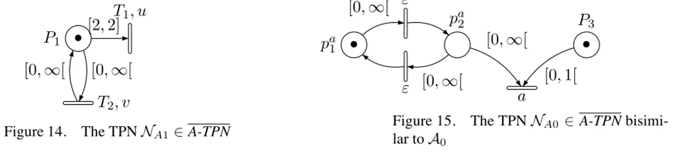
P1 T1, u T2, v [2, 2] [0, ∞[ [0, ∞[ •
Figure 14. The TPN NA1∈ A-TPN
pa 1 pa 2 P3 ε ε a [0, ∞[ [0, ∞[ [0, ∞[ [0, 1[ • •
Figure 15. The TPN NA0 ∈ A-TPN
bisimi-lar to A0
Then, all evolution rules are the same and both are strongly bisimilar.
7 8 Lemma 4.7. (No P-TPN is bisimilar to a A-TPN)
There exists NA1∈ A-TPN such that there is no N ∈ P-TPN weakly timed bisimilar to NA1.
Proof:
The proof is based on Theorem 4.7. The A-TPN NA1 (cf. Fig. 14) is the same net than the T-TPN NT1 (cf. Fig. 12). Obviously, NA1and NT1are (strongly) bisimilar. Then, from Theorem 4.7 that states that there is no P-TPN weakly bisimilar to NT1, there neither is any P-TPN weakly bisimilar to NA1. 78
Lemma 4.8. (No P-TPN is bisimilar to a A-TPN)
There exists NA1∈ A-TPN such that there is no N ∈ P-TPN weakly timed bisimilar to NA1. The proof is the same as for Lemma 4.7.
Theorem 4.9. (A-TPN are strictly more expressive than P-TPN)
P-TPN ⊂≈A-TPN P-TPN ⊂≈A-TPN
Proof:
Obvious from Lemma 4.6, 4.7 and 4.8. 78
4.9. P-TPN #⊆≈T-TPN
According to Corollary 4.2, we have T-TPN #⊆≈ P-TPN. To prove that T-TPN is not more expressive than P-TPN, we prove that the TPN NP of Figure 16 can not be bisimulated by any net of T-TPN. The intuition of the proof is that, in weak semantics, the ) transition can never be forced to be fired. Then, the bisimulation relation should be achieved with some “direct” mapping, which is impossible due to the very different synchronisation rules, like in the strong semantics case.
The Lemma 4.9 proves this “direct” mapping property in a specific case, used in the proof of the Theorem 4.10.
A technical point of the proof could be highlighted: the proof is, like the one of Theorem 4.7, based on the smallest constant of the nets, but, to simplify the notations, the problem can be reduced to a problem on integer, by multiplying by the least common multiple of all denominators.
P1 P2 P3 [0, 1] [0, 1] [0, 1] a b • • Figure 16. A TPN NP ∈ P-TPN
Lemma 4.9. Let us consider a TPN N ∈ T-TPN such that ∀t ∈ T , α(t) ∈ N and β(t) ∈ N. Let us define a state q such that for all run from q, an action b is continuously possible during 0.5 time unit and impossible after 0.5 time unit. Formally it gives :
∀q& st q−−−−→ q("∗,d) &we have "
d ∈ [0, 0.5] ⇒ ∃q& "∗b−−→ d > 0.5 ⇒# ∃q& "∗b−−→
If such state q = (ν, M ) is a state of N then ∃tbwith Λ(tb) = b such that ν(tb) + 0.5 = β(tb) I(tb) is closed on the right α(tb) ≤ β(tb) − 1
The lemma could also states with every value in ]0, 1[, other than 0.5. But for the proof, 0.5 is sufficient.
Proof:
When q is a state, and d a delay (a real number), let q + d denotes the state reached from q by a delay of duration d (because of the time determinism property, it is unique). Formally, it gives : q−→ q + d withd q = (M, ν) and q + d = (M, ν + d)
Because of the weak semantics, the state q + d can always be reached, The proof is decomposed into several steps.
1. Let m be the minimal delay such that no transition met its upper bound between q +m and q +0.5. As q = (M, ν), for each enabled transition t, β(t) − ν(t) is the remaining time before disabling of the transition.
m is then formally defined by : m = max {β(t) − ν(t) M ≥•t and β(t) − ν(t) < 0.5} If the set is empty, m = 0.
As the number of transitions is finite, m obviously exists.
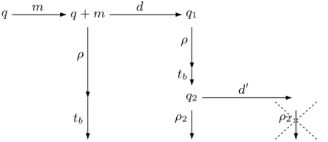
2. From the state q + m, action b is accessible, by a null duration path ρ.
From the hypothesis, there exists a sequence of transitions ρ such that q + m−→ρ tb
−→, with Λ(tb) = b, untimed(ρ) = )∗ and duration(ρ) = 0 (the sequence ρ may be emtpy).
3. The same path ρ can be used a little later
Let d be such that m + d < 0.5. Because of the definition of m, the state q + m + d can be reached without disabling any transition. Let us denote q1 = q + m + d.
By definition of m, every transition firable in q + m is still firable in q1: no upper bound β(t) have been ovelapped by its clock value ν(t). Then, the same transition sequence can be used: q1
ρ −→ tb
q m q+ m d q1 d # ρ ρ tb tb ρ tb
Figure 17. States and path illustrating steps 2, 3, 4 and 5 of the proof of lemma 4.9
q q+ m q1 q2 m d d# ρ ρ tb tb ρ2 ρ2
Figure 18. States and path illustrating step 6 of he proof of lemma 4.9
4. But this path can no more be used once the 0.5 limits have been overlapped: it means a transition
have overlapped its upper bound
Let now be d&such that m + d + d& > 0.5. From our hypothesis, the action b is no more reachable, and then, the path ρtb can no more be used as shown in Fig. 17. It means that there exists a transition t1 in ρtb(i.e. ρtb = ρ1t1ρ2) that was firable from q1and whose upper bound have been overlapped. That is to say a transition t1such that νq1(t1) ≤ β(t1) ≤ νq1+d#(t1).
5. The transition t1was firable from q + m and α(t1) < β(t1).
As ρ1 is in null time, t1is not newly enabled by the firing of a transition in ρ1(Indeed, obviously, β(t1) can not be overlapped without time elapsing). Then t1 is enabled in state q1and then in q and q + m since the marking of these states is the same. Moreover, as t1 is firable from q1 and from q + m we have β(t1) ≥ d > 0 and α(t1) ≤ β(t1) − d < β(t1).
6. The transition tb was firable from q + m and α(tb) < β(tb). If t1 = tb, we can stop (cf previous step).
If not, ρ2 is not empty and ρ2 = ρ&2tb. We can consider q2 defined by q1 ρ1t1
−−−→ q2 (see Fig.18). Because q2is reachable from q with a path of duration m + d < 0.5, the same reasoning can be applied, with ρ&2 instead of ρ. Each ti is enabled in q + m (see previous item). Thus, since the number of enabled transitions in q + m is finite, after a finite n number of steps, we get tn = tb and transition tbwas firable from q + m and α(tb) < β(tb).
νq+(m+d)(tb) ≤ β(tb) ≤ νq+(m+d+d#)(tb)
We have proved νq+m+d(tb) ≤ β(tb) ≤ νq+m+d+d#(tb) ⇐⇒ νq(tb) + m + d ≤ β(tb) ≤ νq(tb) + m + d + d& for all values of d, d& such that m + d < 0.5 and m + d + d& > 0.5. When m + d tends to 0.5 from the left, and m + d + d& tends to 0.5 from the right, both values tends to ν(tb) + 0.5, then ν(tb) + 0.5 = β(tb).
Moreover, because α(tb) and β(tb) are integers, and α(tb) < β(tb) we have α(tb) ≤ β(tb) − 1, and also α(tb) ≤ ν(tb) − 0.5.
7 8 Let us consider the TPN NP ∈ P-TPN of the Figure 16.
Theorem 4.10. There is no TPN ∈ T-TPN weakly timed bisimilar to NP ∈ P-TPN (Fig. 16).
Proof:
The proof is done by contradiction.
Let NP ∈ P-TPN the net of the Figure 16. Assume there exists NT ∈ T-TPN = (P, T,•(.), (.)•, M0, Λ, I) that is timed bisimilar to NP. We denote ∼ the bisimulation relation such that NT ∼ NP.
Let Const = {α(t) > 0, β(t) > 0} be the set of constant of NT and k, be the least common denom-inator of Const.
Let NTk ∈ T-TPN = (P, T,•(.), (.)•, M0, Λ, k.I) be the TPN obtained by multiplying by k all bound α and β of the firing intervals I. The bounds of the firing intervals of NTk are inN.
Moreover NTk is timed bisimilar to the net NPkobtained by the same operation. Let be the run ρk
P = q0 k−0.5 −−−−→ q1
a
−→ q2 in NPk. From q2, every delay of duration d ≤ 0.5 can be followed by a firing of b, and every delay of duration d > 0.5 can not.
Let q0& be the initial state of NTk. By bisimulation assumption, there exists a run ρkT = q&0
("∗,k−0.5) −−−−−−−→ q1& −−→ q"∗a &
2, with q2& = (M2&, ν2&). By bisimulation assumption, q2& respects the hypotheses of Lemma 4.9. It implies that there exists tbwith ΛTk(tb) = b such that αTk(tb) ≤ βTk(tb) − 1.
In q&2, tbis enabled, and tbis firable since 0.5 time unit, that is to say, tb is firable before the firing of the transition of label a, which contradicts the bisimulation assumption. 78 Theorem 4.11. (In weak semantics, T-TPN does not generalise P-TPN)
P-TPN#⊆≈T-TPN
Proof:
This is a direct application of Theorem 4.10. 78
4.10. T-TPN ⊂≈A-TPN
Theorem 4.12. (In weak semantics, A-TPN are strictly more expressive than T-TPN)
Proof:
We already know that T-TPN ⊆≈A-TPN (Lemma 4.4, p. 16).
From the previous Theorem 4.10, there exists NP ∈ P-TPN (Figure 16) that can not be bisimulated by any T-TPN.
From Lemma 4.6, there exists NA∈ A-TPN bisimilar to NP.
Then, NAcan not be bisimulated by any T-TPN, that is to say A-TPN #⊆≈T-TPN. 78
4.11. Sum up
We are now going to sum-up all results in a single location, Figure 19.
T-TPN P-TPN A-TPN T-TPN P-TPN A-TPN #⊆≈(9) !≈ ⊂≈(7) ⊂≈(8) #⊆≈ (3)!≈ ⊂≈(1) ⊂≈(2) #⊆≈(5) !≈ ⊂≈(6) ⊃≈ (4)
Figure 19. The classification explained
(1) and (7) A P-TPN can always be translated into a A-TPN and there exist some A-TPN that can not be simulated by any P-TPN (Theorem 4.9).
(2) A T-TPN can be translated into a A-TPN (Lemma 4.4) and there exist a A-TPN that can not be simulated by any P-TPN (Theorem 4.12).
(3) Corrolary 4.2 states that T-TPN #⊆≈P-TPN, and Theorem 4.11 states the opposite. Both model are incomparable.
(4) The strong semantics of A-TPN strictly generalises the weak one (Theorem 4.3).
(5) Strong and weak T-TPN are incomparable: the weak semantics can not emulate the strong one (Theorem 4.1) but there also exist T-TPN with weak semantics that can not been emulated by any strong T-TPN (Theorem 4.5).
(6) Theorem 4.2 states that P-TPN ⊂≈P-TPN: in P-TPN, the strong semantics can emulate the weak one (Lemma 4.1), but weak semantics can not do the opposite (Theorem 4.1).
(8) A T-TPN can be translated into a A-TPN (Lemma 4.4) and there exists a A-TPN (Lemma 4.5) that can not be emulated by any T-TPN. Then strict inclusion follows (Theorem 4.8).
(9) T-TPN and P-TPN with strong semantics are incomparable: Theorem 4.6 states that there is a
5. Conclusion
Several timed Petri nets models have been defined for years for different purposes. They have been individually studied, some analysis tools exists for some of them, and the users know that a given problem can be modelled with one or the other with more or less difficulty, but a clear map of their relationships was missing. This paper draws most of this map (cf. Fig. 19).
Behind the details of the results, a global view of the main results is the following:
• P-TPN and A-TPN are really close models, since their firing rule is the conjunction of some local clocks, whereas the T-TPN has another point of view, its firing rule taking into account only the last clock;
• the A-TPN model generalises all the other models, but emulating the T-TPN firing rule with A-TPN ones is not possible in practice for human modeller;
• the strong semantics generalises the weak one for P-TPN and A-TPN, but not for T-TPN. The next step will be to study the language-based relationships.
References
[1] Abdulla, P. A., Nyl´en, A.: Timed Petri Nets and BQOs, 22nd International Conference on Application and
Theory of Petri Nets (ICATPN’01), 2075, Springer-Verlag, United Kingdom, 2001.
[2] Aura, T., Lilius, J.: A Causal Semantics for Time Petri Nets, Theoretical Computer Science, 243(2), 2000, 409–447.
[3] Berthomieu, B.: La m´ethode des classes d’´etats pour l’analyse des r´eseaux temporels. Mise en œuvre, exten-sion `a la multi-sensibilisation, Mod´elisation des Syst`emes R´eactifs (MSR’01), Toulouse (Fr), 17–19 Octobre 2001.
[4] Berthomieu, B., Diaz, M.: Modeling and Verification of Time Dependent Systems Using Time Petri Nets,
IEEE transactions on software engineering, 17(3), March 1991, 259–273.
[5] Boyer, M.: Translation from timed Petri nets with interval on transitions to interval on places (with urgency),
Workshop on Theory and Practice of Timed Systems, 65, Elsevier Science, Grenoble, France, April 2002.
[6] Boyer, M., Diaz, M.: Multiple enabledness of transitions in time Petri nets, Proc. of the 9th IEEE
In-ternational Workshop on Petri Nets and Performance Models, IEEE Computer Society, Aachen, Germany,
September 11–14 2001.
[7] Boyer, M., Roux, O. H.: Comparison of the expressiveness w.r.t. timed bisimilarity of k-bounded Arc, Place
and Transition Time Petri Nets with weak and strong single server semantics, Technical Report RI2006-15,
IRCCyN, 2006, (http://www.irccyn.ec-nantes.fr/hebergement/Publications/2006/3437.pdf).
[8] Boyer, M., Roux, O. H.: Comparison of the expressiveness of Arc, Place and Transition Time Petri Nets,
Proceeding of the 28th International Conference on Application and Theory of Petri Nets and Other Models of Concurrency (ICATPN) (J. Kleijn, A. Yakovlev, Eds.), 4546, Springer-Verlag, Siedlce, Poland, june 2007.
[9] Boyer, M., Vernadat, F.: Language and bisimulation relations between subclasses of timed Petri nets with
strong timing semantic, Technical report, LAAS, 2000.
[10] B´erard, B., Cassez, F., Haddad, S., Lime, D., Roux, O. H.: Comparison of Different Semantics for Time Petri Nets, Automated Technology for Verification and Analysis (ATVA’05), 3707, Springer, Taiwan, October 2005.
[11] B´erard, B., Cassez, F., Haddad, S., Lime, D., Roux, O. H.: Comparison of the expressiveness of Timed Automata and Time Petri Nets, 3rd International Conference on Formal Modelling and Analysis of Timed
Systems (FORMATS 05), 3829, Springer, Uppsala, Sweden, 2005.
[12] B´erard, B., Cassez, F., Haddad, S., Lime, D., Roux, O. H.: When are timed automata weakly timed bisimilar to time Petri nets ?, 25th Conference on Foundations of Software Technology and Theoretical Computer
Science (FSTTCS 2005), 3821, Springer, Hyderabad, India, 2005.
[13] Cassez, F., Roux, O. H.: Structural Translation from Time Petri Nets to Timed Automata – Model-Checking Time Petri Nets via Timed Automata, The journal of Systems and Software, 79(10), 2006, 1456–1468. [14] Cerone, A., Maggiolo-Schettini, A.: Timed based expressivity of time Petri nets for system specification,
Theoretical Computer Science, 216, 1999, 1–53.
[15] de Frutos Escrig, D., Ruiz, V. V., Alonso, O. M.: Decidability of properties of timed-arc Petri nets, 21st
International Conference on Application and Theory of Petri Nets (ICATPN’00), 1825, Springer-Verlag,
Aarhus, Denmark, jun 2000.
[16] Hanisch, H.: Analysis of place/transition nets with timed-arcs and its application to batch process control,
14th International Conference on Application and Theory of Petri Nets (ICATPN’93), 691, 1993.
[17] Jones, N. D., Landweber, L. H., Lien, Y. E.: Complexity of Some Problems in Petri Nets., Theoretical
Computer Science 4, 1977, 277–299.
[18] Khansa, W., Denat, J.-P., Collart-Dutilleul, S.: P-Time Petri Nets for manufacturing systems, International
Workshop on Discrete Event Systems, WODES’96, Edinburgh (U.K.), august 1996.
[19] Khanza, W.: R´eseau de Petri P-Temporels. Contribution `a l’´etude des syst`emes `a ´ev`enements discrets, Ph.D. Thesis, Universit´e de Savoie, 1992.
[20] Merlin, P. M.: A study of the recoverability of computing systems, Ph.D. Thesis, Dep. of Information and Computer Science, University of California, Irvine, CA, 1974.
[21] Pezz`e, M.: Time Petri Nets: A Primer Introduction, Tutorial presented at the Multi-Workshop on Formal Methods in Performance Evaluation and Applications, Zaragoza, Spain, september 1999.
[22] Ramchandani, C.: Analysis of asynchronous concurrent systems by timed Petri nets, Ph.D. Thesis, Massa-chusetts Institute of Technology, Cambridge, MA, 1974, Project MAC Report MAC-TR-120.
[23] Sifakis, J.: Performance Evaluation of Systems using Nets, Net theory and applications : Proc. of the
advanced course on general net theory, processes and systems (Hamburg, 1979), 84, Springer-Verlag, 1980.
[24] Srba, J.: Timed-Arc Petri Nets vs. Networks of Timed Automata, Proceedings of the 26th International
Conference on Application and Theory of Petri Nets (ICATPN 2005), 3536, Springer-Verlag, 2005.
[25] Walter, B.: Timed Net for Modeling and Analysing protocols with time, Proceedings of the IFIP Conference
![Figure 1. Priority in strong se- se-mantics [0,2] [1,1] [0,2]uvtFigure 2.Synchronization [1,1] [2,2]tu](https://thumb-eu.123doks.com/thumbv2/123doknet/8162107.274004/9.892.108.778.232.456/figure-priority-strong-se-se-mantics-uvtfigure-synchronization.webp)