HAL Id: hal-01581521
https://hal.archives-ouvertes.fr/hal-01581521
Submitted on 4 Sep 2017
HAL is a multi-disciplinary open access
archive for the deposit and dissemination of
sci-entific research documents, whether they are
pub-lished or not. The documents may come from
teaching and research institutions in France or
abroad, or from public or private research centers.
L’archive ouverte pluridisciplinaire HAL, est
destinée au dépôt et à la diffusion de documents
scientifiques de niveau recherche, publiés ou non,
émanant des établissements d’enseignement et de
recherche français ou étrangers, des laboratoires
publics ou privés.
Improved Local Spectral Unmixing of hyperspectral
data using an algorithmic regularization path for
collaborative sparse regression
Lucas Drumetz, Guillaume Tochon, Miguel Angel Veganzones, Jocelyn
Chanussot, Christian Jutten
To cite this version:
Lucas Drumetz, Guillaume Tochon, Miguel Angel Veganzones, Jocelyn Chanussot, Christian
Jut-ten. Improved Local Spectral Unmixing of hyperspectral data using an algorithmic regularization
path for collaborative sparse regression. ICASSP 2017 - IEEE International Conference on
Acous-tics, Speech and Signal Processing, IEEE, Mar 2017, New Orleans, United States. pp.6190-6194,
�10.1109/ICASSP.2017.7953346�. �hal-01581521�
IMPROVED LOCAL SPECTRAL UNMIXING OF HYPERSPECTRAL DATA USING AN
ALGORITHMIC REGULARIZATION PATH FOR COLLABORATIVE SPARSE REGRESSION
L. Drumetz
a, G. Tochon
b, M.A. Veganzones
c, J. Chanussot
b,d, C. Jutten
aa
Universit´e Grenoble Alpes,
bGrenoble Institute of Technology,
cCNRS, GIPSA-lab, Grenoble, France
dDepartement of Mathematics, University of California, Los Angeles (UCLA), USA
ABSTRACT
Local Spectral Unmixing (LSU) methods perform the unmixing of hyperspectral data locally in regions of the image. The endmembers and their abundances in each pixel are extracted region-wise, instead of globally to mitigate spectral variability effects, which are less se-vere locally. However, it requires the local estimation of the number of endmembers to use. Algorithms for intrinsic dimensionality (ID) estimation tend to overestimate the local ID, especially in small re-gions. The ID only provides an upper bound of the application and scale dependent number of endmembers, which leads to extract irrel-evant signatures as local endmembers, associated with meaningless local abundances. We propose a method to select in each region the best subset of the locally extracted endmembers. Collaborative sparsity is used to detect spurious endmembers in each region and only keep the most influent ones. We compute an algorithmic reg-ularization path for this problem, giving access to the sequence of successive active sets of endmembers when the regularization pa-rameter is increased. Finally, we select the optimal set in the sense of the Bayesian Information Criterion (BIC), favoring models with a high likelihood, while penalizing those with too many endmembers. Results on real data show the interest of the proposed approach.
Index Terms— Hyperspectral imaging, local spectral unmixing, binary partition tree, collaborative sparsity, regularization path
1. INTRODUCTION
Spectral Unmixing (SU) is one of the most important applications in hyperspectral imaging for remote sensing [1]. Because of the limited spatial resolution of hyperspectral images (HSI), observed pixels can account for the contribution of several materials present in the field of view of the sensor during the acquisition. SU is a source separation problem whose goal is to automatically identify the spectral signatures of the materials present in the observed scene (called endmembers) and then to estimate their proportions in each pixel (called abundances). Most SU algorithms assume a Linear Mixing Model (LMM), in which the observations are modeled as linear combinations of the endmembers’ spectra, weighted by the fractional abundances [2]. The abundances are additionally subject to the abundance nonnegativity constraint (ANC) and a sum to one constraint (ASC). Therefore they lie in the probability simplex, and the data lie in another simplex whose vertices are the endmembers. The main two limitations of this approach have been identified as nonlinearities and spectral variability. Nonlinear mixing can hap-pen locally when the incident light undergoes multiple reflections (e.g. in urban scenarios, tree canopies, or particulate media such as This work has been partially supported by the European Research Council under the European Community’s Seventh Framework Programme FP7/2007–2013, under Grant Agreement no.320684 (CHESS project), as well as the Agence Nationale de la Recherche and the Direction G´en´erale de l’Armement, under the project ANR-DGA APHYPIS.
sand) [3]. Spectral variability [4, 5] can affect the endmembers’ sig-natures locally depending on the geometry of the scene (topography and changing illumination conditions) or because of changes in the physico-chemical composition of the materials (e.g. soil moisture content) [6, 7, 8]. Local Spectral Unmixing (LSU) is a technique in which the unmixing is performed in local regions of the image, instead of a whole HSI. The idea is that in smaller local regions, the effects of spectral variability are not so severe. Another motivation is that nonlinear effects are usually very localized in space. The key issue is then to choose the regions on which to perform LSU in an appropriate way. The first methods of the literature to perform the unmixing locally were using sliding windows [9, 10]. Segmentations of the HSI could also be used. The more recent work of [11] uses Binary Partition Trees (BPT) [12] to compute an unmixing-driven hierarchical segmentation of hyperspectral datasets. An optimal par-tition of this hierarchy in the sense of local reconstruction perfor-mance is computed, providing meaningful regions for LSU. How-ever, one of the drawbacks of this approach is that the Intrinsic Di-mensionality (ID) of each region has to be estimated with one of the algorithms of the literature [13], to choose the local number of end-members to use. As shown in [14], the ID can be severely overesti-mated in small regions of the image, or for a large number of spectral bands. Besides, the ID only provides an upper bound of the number of endmembers to use in practice (even for large regions or full im-ages), which is subjective, application and scale dependent. As a result, it often happens that irrelevant endmembers are extracted in many regions, and are associated to very sparse abundance maps. To avoid this, we propose an automatic method to identify and discard irrelevant endmembers in each region during the segmentation step. We make use of collaborative sparsity [15], allowing us to retain only the significant endmember contributions in the region. There is no need to tune any parameters, because we are able to compute a regularization path for the underling optimization problem. The re-mainder of this paper is organized as follows: section 2 introduces in more detail the LSU scheme of [11]. We present our contribution in section 3. Section 4 presents the results of the proposed approach on a real dataset. Finally, section 5 gathers some concluding remarks.
2. BINARY PARTITION TREE BASED LSU In this section, we briefly summarize the BPT-based LSU approach of [11], which is the basis of the present work. The construction of a BPT is conceptually simple: starting from an initial partition of the image (typically an oversegmented partition, obtained using a segmentation algorithm), the two most similar adjacent regions are iteratively merged, building a tree structure. An example is shown in Fig. 1 (a). To obtain an unmixing driven process, we model each region by the set of endmembers extracted by any endmember ex-traction algorithm (EEA) of the literature (here the Vertex Compo-nent Analysis (VCA) [16]). This implies to estimate the ID of each
1 2 3 4 5 1 2 6 5 1 2 7 7 8 9 9 7 8 6 5 1 2 3 4 1 (a) 9 7 8 6 5 1 2 3 4 pruning cut 1 2 7 corresponding partition (b)
Fig. 1. Example of the construction (a) and pruning (b) of a Binary Partition Tree. (a) 100 101 102 103 104 105 0 10 20 30 40 50 60 70
Region size (pixels)
Estimated ID
(b)
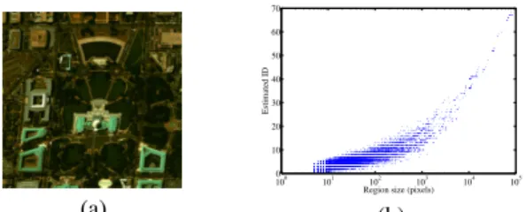
Fig. 2. RGB representation of the Washington DC mall dataset (a), and Local ID of the regions of the BPT (on a logarithmic scale for the x-axis), estimated with the RMT algorithm (b).
region prior to the endmember extraction. One can for instance use the Random Matrix Theory (RMT) based algorithm of [17], with the recommendations of [14] for its use in local settings. The similarity measure used to compare regions is a distance between endmember matrices, proposed in [18]. The abundance maps of each region are also estimated, assuming the LMM holds locally, in each region R:
XR= SRAR+ ER, (1)
We denote by XR∈ RL×NRthe hyperspectral pixels of the region
(L and NRare the number of spectral bands, and the number of
pixels in the region, respectively). SR ∈ RL×dRis the local
end-member matrix, extracted by VCA, and AR ∈ RdR×NR is the
abundance matrix, estimated using the classical Fully Constrained
Least Squares Algorithm (FCLSU) [19]. dRis the estimated ID in
region R. ER∈ RL×NR is an additive noise, usually assumed to
be Gaussian. The BPT is a hierarchical representation of the regions of the image, and in order to get a single partition out of all those possible using the BPT structure, the tree has to be pruned, as shown in Fig. 1 (b). Here, we are able to recover an optimal partition us-ing an optimization process on the hierarchy defined by the BPT. We obtain a partition with a desired number of regions which minimizes an energy based on the reconstruction errors in each region (see [11] for details). In this sense, this segmentation is optimal in terms of SU performance. The local endmembers and abundances can then be recovered for each region of this partition.
3. PROPOSED REGION MODEL 3.1. Motivation
The BPT based LSU scheme described in the previous section has proved useful, but due to the ID overestimation issue in local re-gions, and to the fact that the ID does not always match the expected number of endmembers in an image, the extraction of spurious end-members is frequent. To show this, we built a BPT on the Washing-ton DC mall dataset (shown in Fig. 2 (a)) acquired by the HYDICE sensor, in the visible and near infrared, with a spatial resolution of 2.8m. The initial segmentation was obtained using a mean shift clus-tering algorithm [20], giving an initial partition with 5760 regions. From the BPT, we show in Fig. 2 (b) a plot of the estimated ID as a function of the region size (before the pruning). The estimated ID seems relatively high, up to 70 for the largest regions of the BPT, and regularly over 10 for small regions, (even for regions of 100
Region size: 3460, Estimated ID: 20 Region size: 470, Estimated ID: 9
0.5 1 1.5 2 2.5 0 0.2 0.4 0.6 0.8 1 Wavelength (µm) Normalized Radiance 0.5 1 1.5 2 2.5 0 0.2 0.4 0.6 0.8 Wavelength (µm) Normalized Radiance
Fig. 3. Two regions of a BPT built on the Washington dataset (top row), and the associated extracted endmembers (bottom row). pixels or less). To provide more evidence for this phenomenon, we compare visually in Fig. 3 two regions of the optimal segmentation obtained by keeping around 500 regions. Although a visual inspec-tion can be misleading, we do not expect more than three, perhaps four endmembers in the region on the left, and one or two on the region on the right. However, the estimated IDs were respectively of 20 and 9. The local endmembers extracted by VCA are shown in the bottom row. They clearly show that many signatures are very similar and are probably associated to the same materials. For in-stance, on the left there are at least 6 signatures with a very low spectrum, all associated to shadowed areas of the region. For the rooftop region, only 3 signatures are significantly different from one another in terms of spectral distance (neglecting scaling effects of the signatures). Therefore, most of the abundance maps of these two regions are very sparse (sometimes only non negligible in extremely small regions or isolated pixels), or only there to fit the noise. This means that most of them do not correspond to significant instances of the same materials, and are then not meaningful in terms of spectral variability. However, because they are given the same weight as le-gitimate endmembers in the region model, they can affect the whole BPT construction and pruning. To get better interpretable results in local regions, these dummy endmembers should be discarded in the BPT construction process.
3.2. Collaborative sparsity in LSU
In order to solve this issue, we propose a modified region model for the BPT construction which eliminates the spurious endmembers ex-tracted in a given region. To select the endmembers which should be discarded in the unmixing process, we want to force the ones whose abundance maps are already very sparse or low in most pixels to be zero everywhere, for each region.
To do that, we are going to replace the abundance estimation step within a region with FCLSU by a collaborative sparse unmixing
step [15, 21]. Indeed, the mixed L2,1 norm [22] (||AR||2,1 =
PdR
p=1||aR,p||2, where aR,pis the p
th
row of AR) used in this type
of sparse regression problems encourages row-wise sparsity in the abundance matrix. This means that some endmembers in the region will have zero abundance maps for all the pixels of the region. Then we will only have to discard those from the set of local endmem-bers. Unmixing the region with collaborative sparsity boils down to solving the following convex optimization problem:
arg min AR 1 2||XR− SRAR|| 2 F+ λR||AR||2,1+ I∆dR(AR), (2)
where I∆P is the indicator function of the probability simplex (0
column of AR, and λRis a regularization parameter. This prob-lem can be relatively easily solved using proximal methods, such as the Alternating Direction Method of Multipliers (ADMM) [23]. To use it, we introduce split variables to decouple the different terms in the optimization. We then rewrite problem (2) in the equivalent for-mulation using linear constraints, which is suitable for the ADMM:
arg min AR 1 2||XR− SRAR|| 2 F+ λR||UR||2,1+ I∆dR(VR) s.t. UR= AR, VR= AR. (3)
The ADMM then minimizes an augmented Lagrangian w.r.t. to all the blocks of variables involved, alternatively and iteratively, before
updating the Lagrange multipliers (called CR and DR in
Algo-rithm 1) in a so-called dual update.
However, there are two problems with this approach. The first is that since the linear constraints of the ADMM are only satisfied asymp-totically, in practice the entries of the supposedly discarded rows of the abundance matrix are often not exactly zero, but very small values. Then an arbitrary thresholding step is required to eliminate endmembers with a small contribution [15, 21]. The second is that to obtain the appropriate sparsity level, the regularization parameter
λRneeds to be tuned in every region. A grid search over a set of
parameters in each region would be very computationally costly and would require a criterion to select the best run of the algorithm. We will see that we can find solutions for both issues.
3.3. Obtaining an algorithmic regularization path
In order to tackle both the regularization parameter issue and the inexact sparsity of the collaborative sparse regression at once, we would like to obtain the regularization path of the solution, as a
function of λR. Regularization paths can sometimes be computed
easily, for instance on the LASSO (for Least Absolute Shrinkage Selection Operator) problem [24]. However, for more complex prob-lems, such as ours, there is no way, to our knowledge, to obtain this regularization path easily. A convenient workaround for this is to compute a so-called ADMM algorithmic regularization path, intro-duced in [25]. This approach is able to use the ADMM to quickly approximate the sequence of active supports of the variable of inter-est, when the regularization parameter increases, for certain sparsity regularized least squares problems. Even though there are as of to-day no theoretical guarantees on the efficiency of this algorithm, it was experimentally shown to be able to efficiently approximate the true sequence of active sets on several problems [25], including the LASSO. Here, we propose to extend this algorithm to collaborative sparsity. Since exactly solving the optimization problem for a large number of regularization parameters would be too time consuming, we are more interested in finding the active set of endmembers when the weight of the sparsity term increases w.r.t. this of the data fit term. The idea is, for each region involved in the construction of the BPT, to find a sequence of endmember matrices, whose number
of endmembers are decreasing from dRto zero (when the model is
fully sparse). Each new matrix contains the same endmembers as the previous one, except for one, which is the next endmember to be discarded when the weight of the sparsity term gets more impor-tant. To do that, we modify the ADMM in order to quickly obtain the support of the regularization path, for each region. An iteration of the ADMM is carried out for a very small value of the regular-ization parameter (guaranteeing a fully dense solution). Then, the variables obtained after this iteration are used as a warm start for another iteration with a new slightly higher regularization parame-ter. By repeating this for several iterations with higher and higher
regularization parameters, the split variable UR, which undergoes a
block soft thresholding (the proximal operator of the L2,1norm [23])
becomes increasingly sparse. Since we are using warm starts, and because regularization parameters vary slowly, even if the ADMM is not fully converged at each iteration, the support of the active set
is encoded in UR, often in one iteration only, long before this active
set is propagated to AR(this will be the case only at convergence,
when the constraints of problem (3) are satisfied). With these
mod-ifications, we obtain Algorithm 1. The notation ||UiR||2,0denotes
the number of nonzero rows of the matrix UiR, and ρ is the barrier
parameter of the ADMM. soft·denotes the block soft thresholding
operator with scale parameter in index, and proj∆
dR denotes the
projection on the probability simplex, performed with the algorithm of [26]. These operators are applied columnwise. Here, we are
us-ing a geometric progression for γR(we changed the notation of this
regularization parameter, because we do not completely solve the op-timization problem (3)), whose common ratio is t. This value should be small to approximate the active sets of the regularization path well enough. The regularization space can be explored very quickly
since the algorithm provides at most dRendmember subsets of the
full endmember set extracted by VCA, that need to be tested after
this process. In practice we chose γ0R= 10
−4
and t = 1.04, which
allows γRto sweep from 10−4to 5.104in 500 iterations (less than
what is usually required in practice to reach a fully sparse model).
Data: XR, SR
Result: The sequence of UiR, i = 0, ..., imax
Initialize A0Rand choose γ0Rand t > 0 ;
while ||UiR||2,06= 0 do γi R← tγi−1R ; UiR← softγi R/ρ(A i−1 R − C i−1 R ) ; AiR← (S>RSR+ 2ρIdR) −1 (S>RXR+ ρ(UiR+ Vi−1 R + C i−1 R + D i−1 R )) ; ViR← proj∆dR(A i R− Di−1R ) ; Ci R← Ci−1R + U i R− AiR; DiR← Di−1R + V i R− AiR; i ← i + 1 end
Algorithm 1: Algorithmic regularization path for problem (3). 3.4. Selecting the best model
Using the active sets, we can store a sequence of dRsparser and
sparser candidate endmember matrices (denoted as SiR). The last
step is to select the optimal active set in the sense of some criterion. We used the Bayesian Information Criterion (BIC) [27], which helps choosing from a set of candidate models, by favoring those with an important likelihood, and penalizing those with a high number of pa-rameters. This criterion assumes that the noise is spectrally and spa-tially white, a strong but still widely used assumption. A candidate
model Miis made of one of the SiRand the corresponding estimated
abundances with FCLSU. For our problem, the BIC writes [28]:
BICi= ln(L)Pi+ L ln
||XR− SiRAˆiR||2F
L
!
, (4)
where Piis the number of endmembers in SiR∈ RL×Pi. ˆAiRis the
abundance matrix estimated by FCLSU using the data and the
end-member matrix Si
R. The best model is simply the one minimizing
the BIC value. In our case, to alleviate the computational load, we perform these FCLSU steps from the smallest endmember matrices to the bigger ones, and stop when the BIC value has increased for three consecutive iterations, to avoid performing numerous useless abundance matrix estimations in each region. The flowchart of the proposed region model is shown in Fig. 4.
4. RESULTS
To assess the impact of the proposed modifications to the region model, we built two BPTs on the Washington Mall dataset, one
with-Local endmember set Sequence of local active endmember sets Optimal local endmember set and abundances Region pixels Local ID estimation + VCA endmember extraction
ADMM algorithmic regularization path for Collaborative Sparse
Unmixing Unmixing of the region using all models
Selection of the best model in the BIC sense
Contribution
Fig. 4. Flowchart of the proposed modifications to the region model.
(a) (b) 100 101 102 103 104 105 0 10 20 30 40 50 60 70
Region size (pixels) Estimated ID Number of endmembers retained
(c)
Fig. 5. Optimal segmentations whose number of regions is the clos-est to 500, when no sparsity is considered (a), using the proposed modifications to the region model (b), and number of endmembers in the regions of the BPT with no sparsity (in blue), and with the proposed BPT construction (in red) (c).
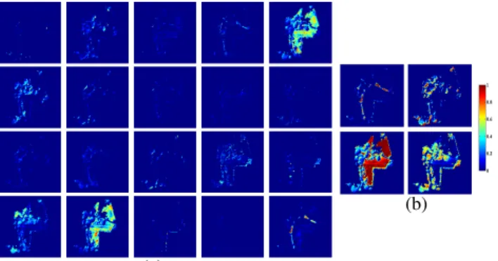
out sparsity, and one with the proposed region model. We show the effect of collaborative sparsity on the local number of endmembers, in Fig. 5 (c). We can see that using the BIC criterion on the sequence of models extracted by the modified ADMM significantly reduces the number of endmembers used in each region. We also computed, in each case, the optimal segmentations whose number of regions is closest to 500 (Fig. 5 (a) and (b)). The regions of these segmenta-tions can correspond to actual structures in the data, but not always, since we are looking for partitions minimizing the RMSE, not for ho-mogeneous regions. The segmentations are relatively similar, with some differences, which shows that we have been able to discard the useless endmembers without significantly impacting the aver-age RMSE. To compare more precisely the local unmixing results on the same regions, we apply the proposed endmember elimination scheme on regions of the BPT obtained without sparsity. We did this on the region on the right of Fig. 3. The average RMSE of this region without sparsity is 0.0061, using 9 endmembers. The proposed ap-proach (for a given run) only retains 3 endmembers, with a RMSE of 0.0064. This shows that we have been able to discard irrelevant end-members by removing the redundant or meaningless information in the region. The proposed region model also significantly impacts the interpretability of the results. For the region on the left of Fig. 3, we show the difference in abundance maps with or without collaborative sparsity (Fig. 6). When no sparsity is applied, at least 8 abundance maps (out of the 20 abundance maps associated to the 20 endmem-bers) have negligible values on almost all the support of the region. Only around 5 abundance maps are really meaningful at the scale of the region. There seems to be 2 instances of grass, 2 instances of trees and one endmember associated to the gravel pathway. With the proposed scheme, only four endmembers are retained: one for grass, two for trees (including one for shadowed parts of the trees), and one for gravel. The different terms involved in the computa-tion of the BIC are displayed in Fig. 7. These plots confirm that
(a)
(b)
Fig. 6. Abundance maps in the region on the left of Fig. 3, without sparsity (a) and with the proposed model selection (b).
5 10 15 100 200 300 400 500 600 700 800 Number of parameters Likelihood term 5 10 15 0 20 40 60 80 100 Number of parameters Parameter term 5 10 15 100 200 300 400 500 600 700 800 Number of parameters BIC (a) 5 10 15 100 200 300 400 500 600 700 800 Number of parameters Likelihood term 5 10 15 0 20 40 60 80 100 Number of parameters Parameter term 5 10 15 100 200 300 400 500 600 700 800 Number of parameters BIC (b) 5 10 15 100 200 300 400 500 600 700 800 Number of parameters Likelihood term 5 10 15 0 20 40 60 80 100 Number of parameters Parameter term 5 10 15 100 200 300 400 500 600 700 800 Number of parameters BIC (c)
Fig. 7. Likelihood (a) and the parameter (b) terms of the BIC (c) for the sequence of endmember matrices obtained with the proposed method, for the region on the left of Fig. 3.
the likelihood term (very related to the mean RMSE in the region) does not decrease much when more than 4 endmembers are retained, while the parameter term increases linearly. The sparsity only kept the most relevant signatures, making the results more easily inter-pretable at the region scale.
It may also happen in some visually relatively homogeneous regions that even with sparsity a significant number of endmembers are re-tained, for instance in the water pond in the center of the upper part of the image. In the most central region, the estimated ID is 5, and no endmember was discarded after the collaborative unmixing. In this region, comprising a shallow water pond (around 50cm deep), and some kind of concrete at the bottom, the mixing process is likely to be highly nonlinear. The BPT approach allowed to isolate this region from the rest of the image, by segmenting it, avoiding the propaga-tion of the errors due to the endmembers of this region. Similarly, in regions which visually correspond to one macroscopic material (e.g. in the region on the right of Fig. 3), several endmembers (around 3 to 6 in this case, depending on the VCA runs) can be retained, be-cause the LMM does not explicitly account for spectral variability, and several endmembers are necessary to fit the data well.
5. CONCLUSION
We have proposed a new region model for local spectral unmixing (LSU) based on binary partition trees (BPT). This model still com-pares the local endmembers extracted in each region, but is able to cope with the extraction of spurious endmembers due to local ID estimation. We get rid of those endmembers by using collaborative sparsity, and avoid parameter tuning in each region by computing an algorithmic regularization path for the resulting optimization prob-lem. We are then able to select the best sparse model by using the Bayesian Information Criterion (BIC). The results show that the pro-posed modifications allow to eliminate the redundant information in each region, without penalizing the unmixing performance. Future work will include an extension of the proposed method for the un-mixing of complete images rather than regions for LSU. In combi-nation with the ideas of [21], a completely blind and parameter free algorithm for simultaneous SU and ID estimation can be designed.
6. REFERENCES
[1] W.-K. Ma, J. M. Bioucas-Dias, J. Chanussot, and P. Gader, “Signal and image processing in hyperspectral remote sens-ing,” IEEE Signal Processing Magazine, vol. 31, no. 1, pp. 22–23, 2014.
[2] J.M. Bioucas-Dias, A. Plaza, N. Dobigeon, M. Parente, Qian
Du, P. Gader, and J. Chanussot, “Hyperspectral unmixing
overview: Geometrical, statistical, and sparse regression-based approaches,” IEEE Journal of Selected Topics in Applied Earth Observations and Remote Sensing, vol. 5, no. 2, pp. 354–379, April 2012.
[3] R. Heylen, M. Parente, and P. Gader, “A review of nonlin-ear hyperspectral unmixing methods,” IEEE Journal of Se-lected Topics in Applied Earth Observations and Remote Sens-ing, vol. 7, no. 6, pp. 1844–1868, June 2014.
[4] A. Zare and K.C. Ho, “Endmember variability in hyperspectral analysis: Addressing spectral variability during spectral un-mixing,” IEEE Signal Processing Magazine, vol. 31, no. 1, pp. 95–104, Jan 2014.
[5] L. Drumetz, J. Chanussot, and C. Jutten, “Endmember vari-ability in spectral unmixing: recent advances,” in Proc. IEEE Workshop on Hyperspectral Image and Signal Processing: Evolution in Remote Sensing (WHISPERS), 2016, pp. 1–4. [6] L. Drumetz, M. A. Veganzones, S. Henrot, R. Phlypo,
J. Chanussot, and C. Jutten, “Blind hyperspectral unmixing using an extended linear mixing model to address spectral vari-ability,” IEEE Transactions on Image Processing, vol. 25, no. 8, pp. 3890–3905, Aug 2016.
[7] S. Henrot, J. Chanussot, and C. Jutten, “Dynamical spectral un-mixing of multitemporal hyperspectral images,” IEEE Trans-actions on Image Processing, vol. 25, no. 7, pp. 3219–3232, July 2016.
[8] P.-A. Thouvenin, N. Dobigeon, and J.-Y. Tourneret, “Hyper-spectral unmixing with “Hyper-spectral variability using a perturbed linear mixing model,” IEEE Transactions on Signal Process-ing, vol. 64, no. 2, pp. 525–538, 2016.
[9] M.A. Goenaga, M.C. Torres-Madronero, M. Velez-Reyes, S.J. Van Bloem, and J.D. Chinea, “Unmixing analysis of a time series of hyperion images over the guanica dry forest in puerto rico,” IEEE Journal of Selected Topics in Applied Earth Obser-vations and Remote Sensing, vol. 6, no. 2, pp. 329–338, April 2013.
[10] K. Canham, A Schlamm, A Ziemann, B. Basener, and D. Messinger, “Spatially adaptive hyperspectral unmixing,” IEEE Transactions on Geoscience and Remote Sensing, vol. 49, no. 11, pp. 4248–4262, Nov 2011.
[11] M. A. Veganzones, G. Tochon, M. Dalla Mura, A. Plaza, and J. Chanussot, “Hyperspectral image segmentation using a new spectral unmixing-based binary partition tree representation,” IEEE Transactions on Image Processing, vol. 23, no. 8, pp. 3574–3589, Aug 2014.
[12] S. Valero, P. Salembier, and J. Chanussot, “Hyperspectral im-age representation and processing with binary partition trees,” IEEE Transactions on Image Processing, vol. 22, no. 4, pp. 1430–1443, April 2013.
[13] A. Robin, K. Cawse-Nicholson, A. Mahmood, and M. Sears, “Estimation of the intrinsic dimension of hyperspectral images:
Comparison of current methods,” IEEE Journal of Selected Topics in Applied Earth Observations and Remote Sensing, vol. 8, no. 6, pp. 2854–2861, June 2015.
[14] L. Drumetz, M. A. Veganzones, R. Marrero G´omez, G. To-chon, M. D. Mura, G. A. Licciardi, C. Jutten, and J. Chanussot, “Hyperspectral local intrinsic dimensionality,” IEEE Transac-tions on Geoscience and Remote Sensing, vol. 54, no. 7, pp. 4063–4078, July 2016.
[15] M.-D. Iordache, J. M. Bioucas-Dias, and A. Plaza, “Collab-orative sparse regression for hyperspectral unmixing,” IEEE Transactions on Geoscience and Remote Sensing, vol. 52, no. 1, pp. 341–354, Jan 2014.
[16] J.M.P. Nascimento and J.M. Bioucas Dias, “Vertex component analysis: a fast algorithm to unmix hyperspectral data,” IEEE Transactions on Geoscience and Remote Sensing, vol. 43, no. 4, pp. 898–910, April 2005.
[17] K. Cawse-Nicholson, S.B. Damelin, A Robin, and M. Sears, “Determining the intrinsic dimension of a hyperspectral image using random matrix theory,” IEEE Transactions on Image Processing, vol. 22, no. 4, pp. 1301–1310, April 2013. [18] M. Grana and M. A. Veganzones, “An endmember-based
dis-tance for content based hyperspectral image retrieval,” Pattern Recognition, vol. 45, no. 9, pp. 3472–3489, 2012.
[19] D.C. Heinz and Chein-I Chang, “Fully constrained least
squares linear spectral mixture analysis method for material quantification in hyperspectral imagery,” IEEE Transactions on Geoscience and Remote Sensing, vol. 39, no. 3, pp. 529– 545, Mar 2001.
[20] D. Comaniciu and P. Meer, “Mean shift: A robust approach toward feature space analysis,” IEEE Transactions on Pattern Analysis and Machine Intelligence, vol. 24, no. 5, pp. 603–619, 2002.
[21] R. Ammanouil, A. Ferrari, C. Richard, and D. Mary, “Blind and fully constrained unmixing of hyperspectral images,” IEEE Transactions on Image Processing, vol. 23, no. 12, pp. 5510–5518, Dec 2014.
[22] M. Kowalski, “Sparse regression using mixed norms,” Applied and Computational Harmonic Analysis, vol. 27, no. 3, pp. 303– 324, 2009.
[23] S. Boyd, N. Parikh, E. Chu, B. Peleato, and J. Eckstein, “Dis-tributed optimization and statistical learning via the alternating direction method of multipliers,” Foundations and Trends in Machine Learning, vol. 3, no. 1, pp. 1–122, 2011.
[24] B. Efron, T. Hastie, I. Johnstone, and R. Tibshirani, “Least angle regression,” The Annals of statistics, vol. 32, no. 2, pp. 407–499, 2004.
[25] Y. Hu, E. Chi, and G. I. Allen, “ADMM algorithmic regu-larization paths for sparse statistical machine learning,” arXiv preprint arXiv:1504.06637, 2015.
[26] L. Condat, “Fast projection onto the simplex and the L1ball,”
Mathematical Programming, pp. 1–11, 2014.
[27] G. Schwarz, “Estimating the dimension of a model,” Ann. Statist., vol. 6, no. 2, pp. 461–464, 03 1978.