HAL Id: hal-01572076
https://hal.archives-ouvertes.fr/hal-01572076
Submitted on 4 Aug 2017
HAL is a multi-disciplinary open access
archive for the deposit and dissemination of
sci-entific research documents, whether they are
pub-lished or not. The documents may come from
teaching and research institutions in France or
abroad, or from public or private research centers.
L’archive ouverte pluridisciplinaire HAL, est
destinée au dépôt et à la diffusion de documents
scientifiques de niveau recherche, publiés ou non,
émanant des établissements d’enseignement et de
recherche français ou étrangers, des laboratoires
publics ou privés.
A Parameter Optimization to Solve the Inverse Problem
in Electrocardiography
Gwladys Ravon, Rémi Dubois, Yves Coudière, Mark Potse
To cite this version:
Gwladys Ravon, Rémi Dubois, Yves Coudière, Mark Potse. A Parameter Optimization to Solve the
Inverse Problem in Electrocardiography. FIMH 2017 - 9th International Conference on Functional
Imaging and Modelling of the Heart, Jun 2017, Toronto, Canada. pp.219-229,
�10.1007/978-3-319-59448-4_21�. �hal-01572076�
A parameter optimization to solve the inverse
problem in electrocardiography
Gwladys Ravon1,2,3∗, Rémi Dubois1,2,3, Yves Coudière1,4,5, Mark Potse1,4,5
1
IHU Liryc, Electrophysiology and Heart Modeling Institute, F-33000 Pessac, France 2
Univ. Bordeaux, CRCTB, U1045, Bordeaux, France 3 INSERM, CRCTB, U1045, Bordeaux, France 4
CARMEN Research Team, INRIA, Bordeaux, France 5 Bordeaux University, IMB UMR 5251, F-33400 Talence, France
Abstract. The main challenge of electrocardiography is to retrieve the best possible electrical information from body surface electrical poten-tial maps. The most common methods reconstruct epicardial potenpoten-tials. Here we propose a method based on a parameter identification prob-lem to reconstruct both activation and repolarization times. The shape of an action potential (AP) is well known and can be described as a parameterized function. From the parameterized APs we compute the electrical potentials on the torso. The inverse problem is reduced to the identification of all the parameters. The method was tested on in silico and experimental data, for single ventricular pacing. We reconstructed activation and repolarization times with good accuracy accurate (CC between 0.71 and 0.9).
1
Introduction
The main challenge of electrocardiography is to retrieve the best possible elec-trical information from body surface elecelec-trical potential maps (BSPM). The most common approach relies on the inverse solution of the Laplace equation in the torso. It reconstructs epicardial potential maps from the BSPM. This technique requires a regularization strategy to deal with the ill-posedness of the problem, and a discretization method to approximate the Laplace equation. A Tikhonov regularization and the Method of Fundamental Solutions (MFS) are commonly used, as proposed by Wang and Rudy [1]. Relevant activation maps can be retrieved from this inverse solution, though it provides signals with a lower amplitude. Nevertheless the reconstruction of accurate activation maps and repolarization maps remains a very challenging problem.
Alternative formulations have been proposed Liu et al. [2] and by Van Oosterom et al. [3], in order to reconstruct directly the activation times (ATs). The method proposed by Liu et al. looks for the three-dimensional activation sequence in the ventricular muscle. The method of Van Oosternom et al. considers both epi-cardium and endoepi-cardium. These approaches still rely on a regularization tech-nique and are not designed to obtain repolarization maps.
We introduce a new technique that aims at recovering both the activation and re-polarization maps on the epicardium. We first focus on single ventricular pacing cases. We propose an approach based on a parameter identification (PI) pro-blem. As epicardial potentials are difficult to parameterize, we rather represent the action potential (AP) as a function of 4 parameters; namely the amplitude, activation time, plateau phase duration and repolarization slope. The final pa-rameter identification problem consists of identifying these 4 space-dependent parameters from the complete BSPM sequence. This method solves the whole electrical sequence: depolarization and repolarization. Since it introduces a pri-ori the shape of the AP, no regularization is needed. The nonlinear least squares parameter identification problem is solved by a gradient method.
The method was tested on both in silico and ex vivo experimental data. We found that activation maps from PI were at least as good as those from the MFS. Accuracy of reconstructed repolarization maps and torso potentials were also discussed.
2
Methods
2.1 Parameterization of the action potential
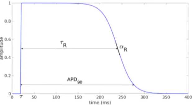
Following the work of Van Oosterom [4] we define the transmembrane potential (TMP) as the function:
Vm(t, x) = AF (α, t − τ )F (−αR, t − (τ + τR)), (1)
where F (α, ζ) = 1
1 + exp−αζ. α is the constant slope of the depolarization.
Its value (3.3 ms−1) is taken from the same study [4]. A is the amplitude, τ the activation time, τR the plateau phase duration and αR the slope of the
repo-larization (see Figure 1). Each of these 4 parameters may be space-dependent. Note that in our study the amplitude does not have physiological value. It is a qualitative parameter made to fit the amplitude of the given BSPM.
2.2 Mapping the TMP to the BSPM
Given the TMP Vmon each point xj of the epicardium, we compute the
extra-cellular potentials:
φe(xj, t) = Vm(t) − Vm(xj, t) j = 1, . . . , NH, (2)
where NHis the number of points on the heart surface. Vm(t) is the spatial mean
of Vmat each time. This formulation is derived from the monodomain model [5].
Finally, we approximate the solution of the Laplace equation far from the heart surface by [6,7]: φT(y, t) = NH X j=1 1 4πkxj− yk φe(xj, t), (3)
where y is any point on the body surface. These φT will be compared to the
BSPM.
2.3 The parameter identification problem
As a consequence we look for the parameter set P = (A, τ, τR, αR) that minimizes
the least squares error
J (P) =1 2 k2 X k=k1 NT X i=1 (φT(yi, tk) − φ?(yi, tk))2, (4)
where (yi)i=1...NTare the NTelectrode locations on the body surface, (tk)k=k1...k2
is the time sequence of interest, and (φ?(y
i, tk)) are the measured BSPM.
However, in order to improve the convergence of the method we make the following choices:
– the amplitude and the repolarization slope are set to a constant over the whole epicardium
– τ and τRare space-dependent. (τj)j and (τR,j)j are taken at the same
loca-tion on the epicardium as (xj)j
– the parameter set is split into the depolarization subset P = (A, (τj)j) and
the repolarization subset P = ((τR)j, αR).
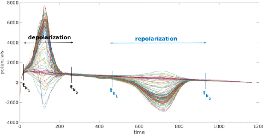
During the depolarization phase of a paced or normal beat we can assume that t τ +τR, so that Vm(t, x) ' AF (α, t−τ ). Hence we solve for P = (A, (τj)j)
in (4) on a time interval [tk1, tk2] that covers the total QRS interval, but contains
no T wave (see Figure 2). Still in order to improve the convergence, we split the identification in two steps: we first identify the constant amplitude A, and then the ATs (τj)j. We apply a standard MFS with a regularization method [1]. This
gives us electrical potentials on the heart surface. We then compute the ATs as the time with the highest negative slope. When we identify the amplitude the parameter set P is simply the singleton {A}, and ATs obtained from the MFS are an input in our PI problem. Once we have this optimized amplitude A? it
becomes an input and the cost function J is minimized for P = ((τj)j).
During the repolarization phase, we solve for P = ((τR,j)j, αR) in (4) on a
time interval [tk1, tk2] that covers the total extent of the T waves (see Figure 2).
We first identify the constant slope (e. g. P = (αR)). The input plateau phase
durations are coarsely determined from the given BSPM. Once we have the optimum α?R we minimize J for P = ((τR,j)j). Optimum A?, (τj?)j and α?R are
an input in this PI problem.
Fig. 2. Example of choice for k1and k2for experimental signals. Each curve represents the signal of one of the torso electrodes.
These four nonlinear least squares problems are solved by the gradient des-cent method. The explicit gradient of the cost function J with respect to the unknown parameters P is calculated analytically. If we wait for the method to converge overfitting occurs. It means that there are small changes in the cost function but the quality of the activation map decreases. To avoid overfitting, we couple the gradient descent method with an early stopping criterion based on the shape of the learning curve. For each gradient descent method, an initial guess is required. For the amplitude, we obtain this guess manually with a dichotomy approach. For the ATs, we use the ATs computed from the MFS. The initial guess for the slope is arbitrarily set to 1. The overall algorithm is summarized below.
Algorithm 1.1
Depolarization phase
1: Standard MFS on interval [tk1, tk2]
2: Compute ATs from MFS solution
3: Gradient descent to optimize the amplitude (MFS ATs as input) 4: Gradient descent to optimize the ATs (optimum A?as input) 5: Gradient descent to optimize the amplitude (optimum τ?as input)
Repolarization phase
1: Input: A?and τ?, from torso signal for τR
2: Gradient descent to optimize the constant slope αR
3: Gradient descent to optimize the (τR,j)j(optimum α?Ras input) 4: Gradient descent to optimize the slope (optimum τ?
Ras input)
3
Results
3.1 In silico data
In order to create in silico testing data, a simulation was run on an anato-mically realistic 3D geometry of the torso, including heart, blood vessels, lungs and skeletal muscle. Each organ had its own conductivity. Propagating action potentials were generated using a monodomain reaction-diffusion model with a Ten Tusscher membrane model [8]. An anisotropic human heart model at 0.2mm resolution was used for this purpose. An anisotropic Laplace equation was solved in the torso volume with a finite difference method [9]. We had ac-cess to the transmembrane potentials on the subepicardium and extra-cellular potentials on the epicardium. ATs were calculated from the epicardial potentials with the same method as the ATs from the MFS solution. Repolarization times were computed from epicardial potentials as the time with the highest positive slope during the repolarization phase.
On the same model anatomy, two different simulations were run: a left ventricu-lar (LV) pacing, and a right ventricuventricu-lar (RV) one. For both cases, we identified our parameters following the algorithm detailed in Algorithm 1.1.
We first looked at the ATs. For the LV pacing the method converged to satisfactory ATs on the whole heart (Figure 3, left). Our method gave a better range of ATs than the MFS. However for both methods the pacing site was not well localized. For the RV pacing, late activations were better reconstructed than the early ones. The correlation coefficient (CC) was the same for both methods but the distribution of points in the scatter plots was different. Indeed for the MFS we observed clustering of points along horizontal lines. This means that there were discontinuities in the distribution of ATs. These discontinuities were not consistent with the reference ATs (Figures 3, right and 4). On the map on the right, discontinuities are clearly visible between the dark blue and light green parts and between the dark green and orange parts.
Fig. 3. Scatter plot of the ATs for in silico data. For each point, the x coordinate is the reference AT and the y coordinate is the corresponding reconstructed AT (PI in red, MFS in blue).
Fig. 4. Activation maps of the RV pacing in silico case.
In Figure 5 we compare APD90 calculated from the reference APs and from the reconstructed ones, for both LV and RV pacing. First of all, we had a larger range of APD90 from the PI, especially for the RV pacing. Moreover, there was a clear difference in the repartition of APD90 between the LV and the RV. This difference was not correctly reconstructed with the PI approach.
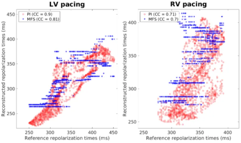
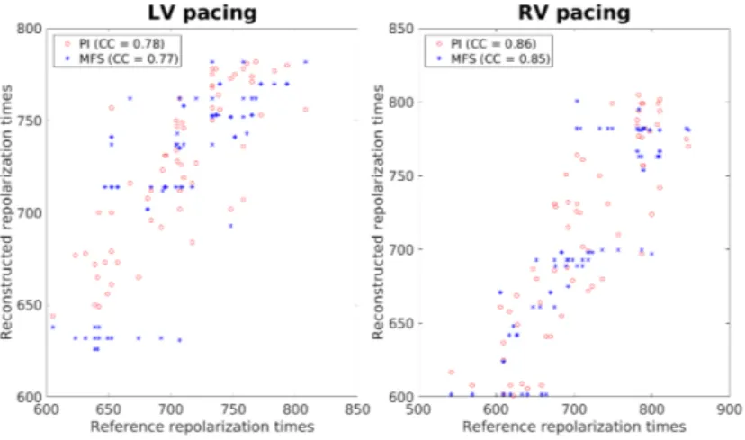
We compare the repolarization times in Figure 6. For the PI, the CC were 0.9 and 0.71 for the LV and RV pacing, respectively. These values were close to those for the MFS but we observed discontinuities in the distribution of points, as for the ATs (see Figure 7). Note that the quality of the reconstruction from the PI method was better for the repolarization times than for the APD90. This can be explained by the fact that if we had an error in the parameter τ , it would imply another error in the parameter τRto fit the repolarization phase correctly.
(a) LV pacing (b) RV pacing
Fig. 5. Comparison of APD90. The reference APD90 are obtained on the subepi-cardium mesh and the reconstructed APD90 on the episubepi-cardium mesh. Anteroposterior view.
Fig. 6. Scatter plot of the repolarization times for in silico data.
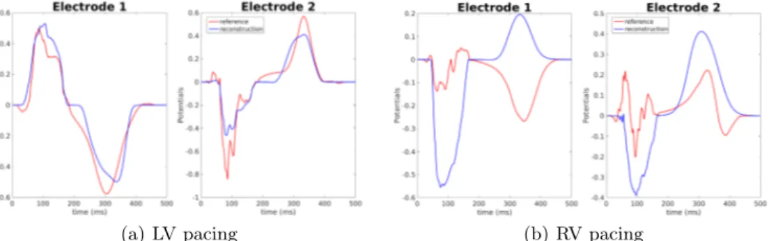
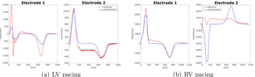
Finally we compare signals on the torso. Reconstructed potentials were com-puted from equations (1), (2) and (3) with the optimized parameters. In both cases the amplitude was optimized to fit the given BSPM. Figure 8 shows given and reconstructed potentials on two torso electrodes. For the LV pacing the am-plitude of the signal was better fitted on the first electrode than on the second. Both depolarization and repolarization phases were quite well identified. These two electrodes were representative for the 252 torso electrodes. For the RV pa-cing, on the same electrodes, the reconstruction was less accurate. Specifically, the repolarization was inverted on the first electrode, while on the second the depolarization was. This was due to the incorrect activation times on the right ventricle. In this case, the chosen electrodes exhibit some of the worst recons-tructed potentials.
(a) LV pacing (b) RV pacing
Fig. 8. Reconstructed potentials for in silico data. Electrode 1: close to the heart, Electrode 2: right hip. Red line: reference BSPM; blue line: reconstructed BSPM.
3.2 Experimental data
Experimental data were obtained from a Langendorff-perfused pig heart with an oxygenated electrolytic solution. Epicardial potentials were recorded with a fle-xible electrode sock (108 electrodes) placed over the epicardium. The heart was placed inside a human-shaped tank. BSPM were recorded from 128 electrodes, simultaneously with epicardial potentials. LV and RV pacing were performed with 1 Hz frequency. We removed signals from bad leads (e.g. not well con-nected) and the baseline. Finally we made a signal averaging over the whole recording to obtain a single beat.
We first looked at the ATs. As for the in silico data, it was difficult to localize the pacing sites precisely. Nevertheless the reconstructed ATs were satisfactory (Figure 9). We noticed a slight improvement of our method compared to MFS for the LV pacing (CC: 0.85 vs 0.82). On the RV pacing (CC: 0.92 vs 0.89) improvement was more obvious when we compared the distribution of points.
Fig. 9. Scatter plot of the ATs for experimental data
Scatter plots of the repolarization times are presented in Figure 10. For both cases, the reconstructed repolarization phase was shorter than the real. The CC were very close for the PI and the MFS but with the PI the distribution was smoother.
Fig. 10. Scatter plot of the repolarization times for experimental data.
Reconstructed potentials are presented in Figure 11. With our method we were able to identify both depolarization and repolarization phases. The am-plitude of the signals was well reproduced thanks to the optimized amam-plitude A?. We did not have any inversions of the T wave. The chosen electrodes were
(a) LV pacing (b) RV pacing
Fig. 11. Reconstructed potentials for experimental data. Electrode 1: close to the heart, Electrode 2: right hip. Red line: reference BSPM; blue line: reconstructed BSPM
4
Conclusion
We presented a parameter optimization method to solve the inverse problem of electrocardiography. Our method relies on a parameterization of the AP. Our main objective was to develop a method that gives precise information on the repolarization phase, in addition to information on the depolarization phase. Moreover, this approach gives access to all the properties of a local AP, like APD90.
We had to make some choices to ensure a good convergence and avoid overfit-ting: constant amplitude and slopes; split the identification process in two steps. Compared to the MFS, our PI gave better activation maps: we obtained a better range of ATs and did not have any artificial discontinuities in the distribution of the ATs on both in silico and experimental data. The method fitted the repola-rization phases quite accurately. However, having a good fit on the repolarepola-rization time could hide an error in the plateau phase duration. Indeed an error in the AT would lead to an error in the plateau phase duration to fit the repolarization phase. Reconstructed torso potentials were close to the measured ones. Espe-cially, optimized amplitude enabled to fit BSPM amplitudes. Moreover, both depolarization and repolarization phases were well caught on all the torso. To improve the quality of the results, we plan to add either the septum or the endocardium into the geometry. Another development will be to consider piece-wise constant amplitudes and repolarization slopes, instead of constant over the whole epicardium.
Acknowledgments
This study received financial support from the French Government as part of the “Investments of the Future” program managed by the National Research Agency (ANR), Grant reference ANR-10-IAHU-04. This work was granted access to the HPC resources of TGCC under the allocation x2016037379 made by GENCI.
References
1. Y. Wang, Y. Rudy: Application of the method of fundamental solutions to potential-based inverse electrocardiography. Ann. Biomed. Eng. 2006; 34:1272-1288
2. Z. Liu, C. Liu, B. He: Noninvasive reconstruction of three-dimensional ventricu-lar activation sequence from the inverse solution of distributed equivalent current Density. IEEE Trans. Med. Imag., vol 25, 1307-1318 (2006)
3. A. van Oosterom, T. Oostendorp: On computing pericardial potentials and current densities in inverse electrocardiography. J. Electrocardiol. 25S:102–106 (1993) 4. A. van Oosterom, V. Jacquemet: A parameterized description of transmembrane
potentials used in forward and inverse procedures. Int. Conf. Electrocardiol. 6, 5-8 (2005)
5. S. Labarthe: Modélisation de l’activité électrique des oreillettes et des veines pul-monaires. Thesis, University of Bordeaux (2013)
6. J. Malmivuo, R. Plonsey: Bioelectromagnetism: principles and applications of bio-electric and biomagnetic fields. Oxford University Press, USA (1995)
7. P. W. Macfarlane, A. van Oosterom, O. Pahlm, P. Kligfield, M. Janse, J. Camm: Comprehensive Electrocardiology. Springer London (2010)
8. K. H. W. J. ten Tusscher, D. Noble, P. J. Noble, A. V. Panfilov: A model for human ventricular tissue. Am. J. Physiol. H., vol 286 (2004)
9. M. Potse, B. Dubé, A. Vinet: Cardiac anisotropy in boundary-element models for the electrocardiogram. Med. Biol. Eng. Comput., 47(7), 719-729 (2009)