Publisher’s version / Version de l'éditeur:
Vous avez des questions? Nous pouvons vous aider. Pour communiquer directement avec un auteur, consultez la première page de la revue dans laquelle son article a été publié afin de trouver ses coordonnées. Si vous n’arrivez pas à les repérer, communiquez avec nous à [email protected].
Questions? Contact the NRC Publications Archive team at
[email protected]. If you wish to email the authors directly, please see the first page of the publication for their contact information.
https://publications-cnrc.canada.ca/fra/droits
L’accès à ce site Web et l’utilisation de son contenu sont assujettis aux conditions présentées dans le site LISEZ CES CONDITIONS ATTENTIVEMENT AVANT D’UTILISER CE SITE WEB.
Student Report (National Research Council of Canada. Institute for Ocean Technology); no. SR-2008-04, 2008
READ THESE TERMS AND CONDITIONS CAREFULLY BEFORE USING THIS WEBSITE.
https://nrc-publications.canada.ca/eng/copyright
NRC Publications Archive Record / Notice des Archives des publications du CNRC : https://nrc-publications.canada.ca/eng/view/object/?id=b9c9cb92-f743-4acc-be12-ab4cfd2eedbe https://publications-cnrc.canada.ca/fra/voir/objet/?id=b9c9cb92-f743-4acc-be12-ab4cfd2eedbe
NRC Publications Archive
Archives des publications du CNRC
For the publisher’s version, please access the DOI link below./ Pour consulter la version de l’éditeur, utilisez le lien DOI ci-dessous.
https://doi.org/10.4224/8895338
Access and use of this website and the material on it are subject to the Terms and Conditions set forth at
Automated image analysis for marine icing events
National Research Council Canada Institute for Ocean Technology Conseil national de recherches Canada Institut des technologies oc ´eaniques
Student Report
SR-2008-04
Automated Image Analysis for Marine Icing Events
W. Bruce
April 2008
DOCUMENTATION PAGE REPORT NUMBER SR-2008-04 NRC REPORT NUMBER SR-2008-04 DATE April 18, 2008
REPORT SECURITY CLASSIFICATION
UNCLASSIFIED
DISTRIBUTION
UNLIMITED
TITLE
Automated Image Analysis for Marine Icing Events AUTHOR(S)
Wayne Bruce
CORPORATE AUTHOR(S)/PERFORMING AGENCY(S)
IOT/NRC
PUBLICATION
SPONSORING AGENCY(S)
IOT/NRC
IOT PROJECT NUMBER NRC FILE NUMBER
KEY WORDS Marine Icing PAGES 45, Apps. A-C FIGS. 12 TABLES SUMMARY
Describes an automated approach for detecting ice thickness on vessels. Uses Marine Icing Monitoring System and Python to calculate the total ice accumulation and rate of increase during icing events on the Atlantic Kingfisher
ADDRESS National Research Council
Institute for Ocean Technology Arctic Avenue, P. O. Box 12093 St. John's, NL A1B 3T5
National Research Council Conseil national de recherches Canada Canada
Institute for Ocean Institut des technologies Technology océaniques
AUTOMATED IMAGE ANALYSIS
FOR MARINE ICING EVENTS
SR-2008-04
Wayne Bruce
Table of Contents
1.0 Introduction ... 1
2.0 Ice Accumulation ... 1
2.1 Marine Icing Spray... 2
3.0 Marine Icing Monitoring System... 3
4.0 Image Analysis ... 5 4.1 Positions ... 5 4.2 Image Processing ... 7 4.3 Edge Detection ... 9 4.4 Calibration ... 10 4.5 Sub-Pixels ... 10 4.6 Generated Images ... 12 4.7 Elliptical Structures ... 13
5.0 Ice Progression Graph ... 14
5.1 Features ... 15
5.2 Relationships ... 16
6.0 Conclusion ... 17
Table of Figures
Figure 1: Icing event on the Kingfisher ... 2Figure 2: Splash occurred against the Kingfisher ... 3
Figure 3: MIMS cameras on the Caribou ... 4
Figure 4: Icing and precipitation on MIMS camera ... 5
Figure 5: Positions used during automated analysis ... 7
Figure 6: (a) Icing image rotated (b) rotated and converted to greyscale ... 8
Figure 7: Generated image of the railing with image enhancements... 9
Figure 8: Before sub-pixel method was incorporated into edge detection ... 11
Figure 9: After sub-pixel method incorporated... 12
Figure 10: Generated image of linear structure (black pole structure)... 13
Figure 11: Generated image of the elliptical structure ... 14
Figure 12: Graph generated from Dec. 29 icing event... 15
Appendices
Appendix A: Python Code for Automated Image Analysis
Appendix B: Sample Analysis Pictures for Icing Event (Dec. 29, 2006) Appendix C: Icing Event Figures for Ice Accumulation
Automated Image Analysis for Marine Icing Events
1.0 Introduction
This report will focus on the analysis of ice accumulation using the Marine Icing Monitoring System (MIMS). Ice build-up continues to be a concern for offshore structures and vessels during the winter months. Python, a programming language, along with images from the MIMS technology uses an automated approach to calculate the rate and thickness of ice during icing events. Currently, the program investigates icing events occurring in the 2006/2007 winter on the Atlantic Kingfisher, an offshore supply vessel providing support for Petro-Canada’s Terra Nova project. MIMS, developed by the Institute for Ocean Technology, continues to try and improve this technology and increase safety conditions during icing events.
2.0 Ice
Accumulation
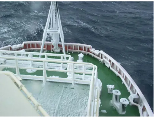
Ice accumulation on vessels can be a dangerous and cause both operation and safety problems if the issue is not monitored. The accumulation is caused by precipitation and marine icing spray under cold weather conditions. With significant amounts of ice build-up, the vessel’s weight can increase dramatically. This problem can result in stability issues as the centre of gravity of the vessel may be altered. Figure 1 shows large amounts of ice on the Atlantic Kingfisher during the winter of 2006/2007. This type of accumulation can become a major hazard to the standard operations of the vessel. With the potential to capsize vessels, icing is a danger that must be monitored during the winter.
Figure 1: Icing event on the Kingfisher
2.1 Marine Icing Spray
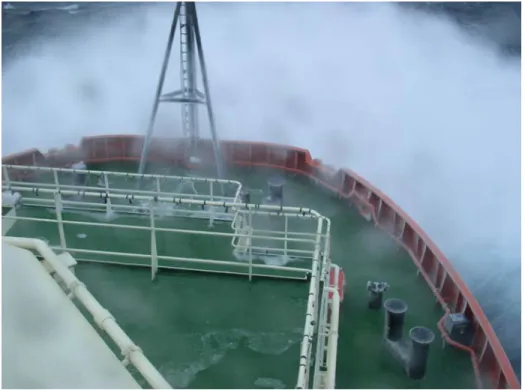
Marine icing spray refers to large sprays of water onto the deck of the ship. It is caused by waves crashing into the hull of the ship under certain weather conditions. Marine icing spray, as shown in Figure 2, can produce large amounts of water on the vessel’s deck, as the excess water will cause icing on susceptible areas of the vessel. High wind speed of approximately 9 m/s is needed to create sufficient waves (1m or higher) for the icing spray and a temperature of –10 °C is sufficient for icing to occur on the vessel. Under these conditions, marine icing spray is prone to create ice build-up and safety issues.
Figure 2: Splash occurred against the Kingfisher
3.0 Marine Icing Monitoring System
To monitor the icing events that occur on vessels, the Institute for Ocean Technology (IOT) developed the Marine Icing Monitoring System (MIMS). With the use of this technology, ice accumulation can be continuously observed to avoid problems that can occur during these circumstances.
MIMS technology is comprised of two cameras connected to a CPU (see Figure 3). The stationary cameras are located at the starboard and port sides of the vessel facing the front of the vessel. Each camera is programmed to take a picture in intervals of 12 minutes. The timing of both cameras is offset from each other creating one picture every 6 minutes. As well, the system includes a metal casing around the camera and a well-insulated area for all electronic components during marine conditions.
For monitoring purposes, a satellite phone was established to control the technology from IOT. The capabilities of the phone include zooming the camera
in and out and downloading images captured by the technology. Thumbnail images are often downloaded for monitoring since large full-scale images take great deal of time to produce. Instead, these images are retrieved from the vessel after the winter season.
Figure 3: MIMS cameras on the Caribou
The first Marine Icing Monitoring System was installed on Marine Atlantic’s ferry, the MV Caribou. This system was used to gain information on the system’s ability to tolerate the environmental conditions. From observations of the first cameras, additional heaters needed to be installed as the camera window continued to freeze during icing events. Adjustments were made to improve the second MIMS installed on the Atlantic Kingfisher. Visibility has increased from the first MIMS but some ice can still form on the camera window (shown in Figure 4). The images from the second MIMS are used for the automated analysis during the 2006/2007 winter. Currently, as of October 2007, these cameras have been moved to a similar oil supply vessel called the Atlantic Eagle. Seals, antenna, and power supply all needed to be replaced before installation.
Figure 4: Icing and precipitation on MIMS camera
4.0 Image
Analysis
The images collected using the MIMS technology can be analyzed further to incorporate the amount and rate of ice accumulation during icing events. Python, an object-oriented programming language, is used for analysis in an automated approach. The program uses edge detection techniques to find the width of particular structures for each image during the icing event. By comparing these measurements to the actual width found with no ice, the computer can output the ice thickness. Currently, the analysis has been conducted for icing events occurring on the Atlantic Kingfisher in December 2006 – February 2007. The program incorporates positions from the fixed images of the Kingfisher, however, the method could be modified for other vessels in the future.
4.1 Positions
The positions for analysis have been chosen to correspond with the techniques used in the program. There are many factors that make one position more
suitable than another to analyze. For example, linear structures result in more accurate edge detection calculations than rounded or elliptical structures. This result is caused by the edge detection method chosen for analysis. The method focuses on pixels of the image in a linear approach causing rounded structures to be less accurate.
As well, positions with vertical members have ice accumulation that is more uniform than horizontal structures. During icing events, horizontal structures, such as the white railing shown in Figure 11, will create icicles. The analysis can become flawed at these positions as it becomes difficult to find ice thickness.
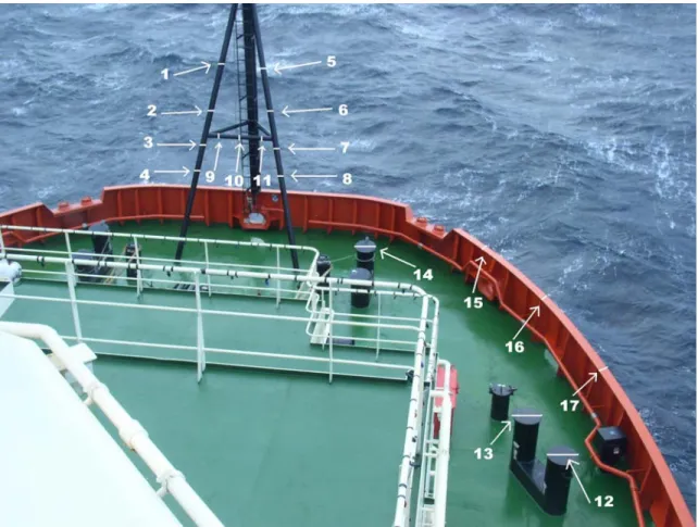
There have been 17 positions chosen for analysis during the icing events. As you can see from the figure below, the majority of which are located on the black pole structure. This structure appeared to give the most accurate results when computing the ice thickness on the vessel. With so many positions on this structure, relationships with respect to height and distance can be observed from analysis. As well, significant ice build-up has been observed on the black circular structures and the railing of the vessel in which three positions each have been analyzed.
Figure 5: Positions used during automated analysis
4.2 Image Processing
Each image in the icing event must undergo the same filters and enhancements to ensure the best possible results. When conducting image processing in Python, a new module called Python Imaging Library (PIL) must be imported into the script. PIL adds image-processing capabilities to your interpreter and contains all basic commands needed to manipulate your image. The commands are created to simplify programs and reduce the time it can take to run large self-written modules for images.
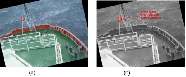
When the image is uploaded, it is rotated by a particular amount calculated for each position. This occurs so that the structure analyzed is in a vertical position required for edge detection. Next the image is changed completely to greyscale
(see Figure 6). A greyscale image is easier to process as all pixels in the image can be related using the same numerical scale (black = 0 and white = 255). After these processes, the program uses the crop command to focus on the position that is being calculated. The cropped image is modified to a size that will exclude as much noise and possible edges that can interfere. However, ice growth on the structure must be accounted for when determining a convenient size for the newly cropped image. This order of commands is created through testing of different configurations. The image has a greater clarity if the rotation and greyscale command precedes the cropping of the image.
(a) (b)
Figure 6: (a) Icing image rotated (b) rotated and converted to greyscale
Following these modifications, the image undergoes enhancements to continue to make the image clear for processing. Auto contrast is one command that is used with a particular cut off level. Any greyscale pixel that is above or below the percentage used for cut off will be changed to black or white, respectively. Another important command is a Median Filter, used for reducing noise in the image. The program uses a 3x3 filter, which analyzes the pixels in that window size. The value of each pixel is examined and all pixels are changed to the median value of the area. This will help avoid speckle noise that can occur in the image. Other commands that can be used for noise reduction include smoothing or blurring the image as well as an EDGE_ENHANCE command to expose the edges better. However, from further tests, these commands were not included in
the script. These seemed ineffective or did not improve the calculated widths of the structure. The final image modification is a command known as FIND_EDGES. With this command, the image is converted to black and white as the greyscale pixels are changed to whichever extremity is closer. This results in a black image with edges surfacing as white pixels.
The image processing has changed slightly depending on the particular position during the calculation. For example, color can be a factor for the railing because it has a distinctive red color compared to the positions on the black structure. This creates a lighter image when the greyscale is incorporated. Therefore, changes have been made to create the most accurate results. Image processing for edge detection can be created with only a small amount of code with the use of Python Imaging Library. This module has made very technical processes into conveniently small commands for the script.
Figure 7: Generated image of the railing with image enhancements
4.3 Edge Detection
When the image has gone through the image processing steps, the program is ready to detect its edges. Images are comprised of pixels, single points in the
graphic image that occupy a definable area. Each pixel is represented in a numerical scale which can be anywhere between black at 0 or white at 255. The values of each column of pixels in the image are averaged and compiled in a table in an Excel spreadsheet for easy access. The program begins a loop process at the left side of the image and continues through each column until it has found the maximum value for half of the columns. The loop will end at this maximum and this pixel value is determined as the left edge of the structure. The same method is used for the right edge as the program checks from right to left of the image for the maximum. The subtraction of the right and left edges calculates the width of the structure in pixels.
4.4 Calibration
The width at each position analyzed has no significant meaning without any calibrations. The positions used have been manually measured on the Kingfisher vessel to use for this calibration process. The program is run through images with no ice accumulation to calculate the initial pixel width. The calibration factor of each position is equal to the actual width of structure (in centimetres) divided by the pixel width of the positions with no ice. This value will increase as positions are farther away from the camera. With a list of calibration factors multiplied by each position, respectively, the calculated widths can be displayed in centimetres. The ice accumulation can now be related in actual measurements that are suitable for the analysis.
4.5 Sub-Pixels
A problem that occurred after observing the analysis included frequent time intervals with the exact same width as the icing event progressed. This occurrence was not due to the lack of ice accumulation during these images. The problem is a result of the edge detection process whereby the calculated width can only be from one pixel to another (Ex. From the black structure each measurement is at least 0.68cm apart). The result is data that becomes fixed at
the same value for a period of time instead of steadily increasing data. To resolve this problem, the measured widths must be calculated in a sub-pixel level. The edge detection process discussed earlier needed small adjustments to achieve this goal. Instead of averaging pixel values of each column, you could use the same method numerous times with a selected amount of rows (used sections of 5 rows). By using the edge detection technique several times and averaging these values found, the data set becomes more accurate for the ice thickness analysis. The data shows an improved uniform increase as expected for actual conditions. As well, necessary error factors have been implemented to this list of edge values to ensure that flawed values do not affect the analysis.
Figure 9: After sub-pixel method incorporated
4.6 Generated Images
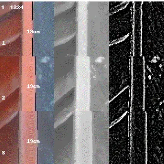
To assist with the analysis of the icing event, the program generates a progressive image to incorporate three stages of the image analysis. All three sections of the image are the cropped image at the particular position that is analyzed. The first section includes the image cropped and rotated while the second contains the image changed to greyscale with the other enhancements implemented by the program. Finally, the last section includes all edge commands and the final appearance that the edge detection will use for calculations. As well, the script produces lines as markers for the left and right edge of the structure. These appear on the first section as vertical lines for the linear structures and horizontal lines for the elliptical. These lines give an indication on whether the program is running properly and detecting the edges well. It also gives the ability to show the ice accumulation increase with each new
image. The images include reference number, time of day, and position number. Another property that has been included in the images is whether or not the detection process could not find an edge. If this is the case, the program will output ‘Could not find edges’ directly on the photo. This width value for the particular position is removed from the data. The indication creates further inspection and helps the detection process. Often you can reference back to the original image to check if any precipitation on the camera is the problem or if the process is not responding well.
Figure 10: Generated image of linear structure (black pole structure)
4.7 Elliptical Structures
The Edge detection method that has been used is ideally suited for linear structures such as black pole structure in the image. However, from inspection, there is significant ice accumulation on the circular black covers as shown in Figure 11. This accumulation warrants analysis at these positions. Three positions have been chosen to analyze with the program. Unfortunately, the techniques previously used for the linear structures do not accurately determine
the edges of the elliptical shape. To resolve this problem, the program has been adjusted with small changes to the edge detection. Instead of evaluating all rows of pixels, the program will average the pixel values of several rows in the middle of image. This will determine the rounded edge more effectively from the elliptical shape. This method works significantly better than the original, but the linear structures continue to show a more accurate result.
Figure 11: Generated image of the elliptical structure
5.0 Ice Progression Graph
With the addition of the matplotlib extension to Python, the program is given graphing capabilities to help display the ice analysis (see Appendix C). As shown in Figure 12, the script will output and save a graph displaying all the necessary calculations of the icing event in an organized manner (see Appendix B for additional graphs of each position during the December 29, 2006 icing event).
Figure 12: Graph generated from Dec. 29 icing event
5.1 Features
The graph includes a scattered plot of the width of each structure as the icing event progresses. A line of best fit is incorporated with respect to the data using standard commands in Python. The accuracy of this line is given in the top left corner of the graph as standard deviation. The residual standard deviation represents the average distance that each point is away from the best-fit line. As well, the ice thickness is calculated from the data by comparing the width of the standard structure with no ice and the icing width after the accumulation. The third calculation given at the top of the graph is the rate at which the ice is growing. This refers to the thickness of ice divided by the length of time for the icing event (five images are captured during one hour).
To increase the accuracy of the results, an error calculation is incorporated to avoid flawed data points (shown in Python Code, Appendix A). Edges that are not detected correctly can lead to a best-fit line that does not represent the entire data set well. By using the error formula, these points are removed from the data by comparing all points to the median value.
5.2 Relationships
From inspection of the graphs generated by the program, the most accurate data is retrieved from the black pole structure (see Appendix C for all positions). These positions have a smaller residual standard deviation than other position as the values are more closely related to the line of best fit. However, the horizontal pole of the black structure (positions 9, 10, and 11) does not calculate with the same accuracy. This is caused by the fact that some icicles have formed on the bottom of the pole creating ice build-up that is not uniform and difficult to calculate.
In addition to the black structure, the data from the railing positions were accurate with small deviation. However, more flawed values were removed and resulted in a smaller data set. These positions create better results than the elliptical data, as the computer often cannot detect the round edge effectively.
Another trend that can be observed from the data collected is with respect to the height and distance from the exterior of the vessel. As the height of the position decreases (seen in positions 1-4 and 5-8 of Figure 5), the ice accumulation increases. This occurrence is based on the marine icing spray as the lower positions of the structure tend to be sprayed in greater amounts. As well, the railing shows a relationship with the bow of the vessel. There is significantly greater ice accumulation the closer to the
bow since this is the part of the vessel, which the icing spray initially originates (positions 15, 16, and 17 of railing). Distance also plays a role with the white poles displayed in the image since they seem to be too far from the hull of the vessel to get sufficient icing spray to create accumulation.
6.0 Conclusion
The MIMS technology continues to be employed on the Atlantic Eagle as it captures a large amount of images during each winter. The images give the ability to monitor and research icing on offshore vessels and have the potential to avoid dangerous situations.
With the use of Python, ice accumulation and the rate of growth has been calculated in an automated approach. The accuracy of the automated analysis continues to improve and demonstrate the positions susceptible to icing. As MIMS and the detection methods develop, it can be a significant safety feature for vessels. Monitoring these icing events is necessary for all vessels travelling in waters that are prone to marine icing.
References
Guido van Rossum. Python Tutorial. February 21, 2008. <http://docs.python.org/tut/tut.html>
Python Imaging Library. May 6, 2005. Handbook reference. Viewed January
2008. <http://www.pythonware.com/library/pil/handbook/index.htm>
Cluett, D. Automated Analysis of Marine Icing Images. Institute for Ocean
Technology. 2007. SR-2007-02
Gibling, L. Marine Icing Events: an Analysis of Images Collected from the Marine
Icing Monitoring system (MIMS) Institute for Ocean Technology. 2007
Appendix A
Python Code for Automated
Image Analysis
import Image # PIL Python Image Library import ImageOps import ImageFilter import ImageDraw import ImageFont import glob, os import csv
from pylab import * frame = 100000
calib = (0.68, 0.68, 0.68, 0.68, 0.68, 0.68, 0.68, 0.68, 0.68, 0.68, 0.68)
boxS = (60,80) # size of image segment
boxR = [12.6, 12.6, 12.6, 12.5, -9.5, -9.6, -9.6, -9.6, 94, 94, 94] # rotation of image segment
boxO = [(575,350), (575,400), (575,575), (575,630), (950,225), (950,275), (950,425), (950,500), (725,1230), (725,1170), (725,1113)
] # location of corner of image segment after rotation cmlist = [[] for i in range(len(boxR))]
boxesSize = [(a[0], a[1], a[0]+boxS[0], a[1]+boxS[1]) for a in boxO] holdSize = [ 0, 0 , boxS[0]*3, boxS[1]*len(boxO)] # output image gif cnt = 1
fo = csv.writer(open("E:\Icing Event\icing.csv", 'wb')) fof = csv.writer(open("E:\Icing Event\icingNum.csv", 'wb')) col = [(' ')]*(3) # output data
for infile in glob.glob("E:\\Icing Event\\Icing Pics\\J*.jpg"): filepath, filename = os.path.split(infile)
filename, ext = os.path.splitext(filename) results = [filename] # list of file names
results.append(cnt) # append counter to list of file names im = Image.open(infile) # open image
hold = im.crop(holdSize) # create image to hold visual results
for i, box in enumerate(boxesSize): # for each area to analyze region = im.rotate(boxR[i], resample=2) # rotate image hold.paste(region.crop(box), (0, boxS[1]*i)) # save cropped original #region = region.crop(box) region = ImageOps.grayscale(region) #region = region.filter(ImageFilter.SMOOTH) #region = region.convert('L') #region = region.filter(ImageFilter.BLUR)
region = ImageOps.autocontrast(region, cutoff=10) region = region.filter(ImageFilter.MedianFilter(3)) region = region.filter(ImageFilter.SMOOTH) region = ImageOps.autocontrast(region, cutoff=3) #region.show()
#edge = region.filter(ImageFilter.EDGE_ENHANCE) edge = region.filter(ImageFilter.MedianFilter(3)) edge = edge.filter(ImageFilter.FIND_EDGES)
edge = ImageOps.autocontrast(edge, cutoff=2) #edge.show()
edge = edge.crop(box)
hold.paste(region.crop(box),(boxS[0], boxS[1]*i)) # save processed segment
hold.paste(edge,(boxS[0]*2, boxS[1]*i)) # save edge segment
width,height = edge.size # get the size of the image temp = [0]*width # temp list to hold average values string = ''
data = list(edge.getdata()) # convert image to list of values first1 = []
last1 = []
for n in range(height/5): rge_htx = (0 + 5*n) rge_hty = (5 + 5*n)
for j in range(width): # average values for each column for k in range(rge_htx,rge_hty):
temp[j] += float(data[k*width+j]) temp[j] = temp[j]/(height/5)
if i == 0: # for first segment output column averages col[1] = j
col[2] = '%5.1f' % (temp[j]) col[0] = cnt
fo.writerow(col)
peak = int(max(temp[5:-5])*0.7) # define peak value as 70% of max
for k in range(5, width/2): # find left edge if peak < temp[k]:
first1.append(k-1) break
for k in range(width-5, width/2, -1): # find right edge if peak < temp[k]:
last1.append(k+1) break
## print first1, last1
if len(first1) != 0 and len(last1) != 0: error = (first1 - mean(first1))**2 ermedian = median(error) * 1.5 g = 0 for f in range(0,len(first1)): if error[f] > ermedian: first1 = delete(first1, [g]) g = g-1
elif error[f] < ermedian/2.5: first1 = delete(first1, [g])
g = g-1 g += 1
error = (last1 - mean(last1))**2 ermedian = median(error) * 1.5 g = 0 for f in range(0,len(last1)): if error[f] > ermedian: last1 = delete(last1, [g]) g = g-1
elif error[f] < ermedian/2.5: last1 = delete(last1, [g]) g = g-1 g += 1 first = mean(first1) last = mean(last1) ## print first1,last1 ## print first,last pixelwidth = (last-first) draw = ImageDraw.Draw(hold) cmwidth = calib[i] * pixelwidth
if len(first1) == 0 or len(last1) == 0:
draw.text((5, boxS[1]*i+20), 'Could not find edges') else:
cmlist[i].append(cmwidth)
results.append(pixelwidth) # append width of edges to results
text = ' %s ,%3d, %3d, %3d' % (filename, pixelwidth, int(first), int(last))
string = '%2.1f' % (cmwidth) + 'cm'
pos = (int(boxS[0]/3), int(boxS[1]*i+boxS[1]/2)-1) draw.text( pos, string) # write edge width on image topline = int(boxS[1]/3+boxS[1]*i) botline1 = int(boxS[1]*2/3+boxS[1]*i) botline2 = int(boxS[1]+boxS[1]*i) draw.line(((first,boxS[1]*i), (first,topline)),fill=256,width=1) draw.line(((first,botline1), (first, botline2)),fill=256,width=1) draw.line(((last,boxS[1]*i),(last,topline)),fill=256,width=1) draw.line(((last,botline1),(last,botline2)),fill=256,width=1) # displays text for position counter, image counter, and time of each image for h in range(0,len(boxR)): string1 = (('%d' % (h+1)), ('%d' % (cnt)), (infile[-9:-5])) pos = ((5, boxS[1]*h+70), (4,5), (20,5)) for g in range(0,len(string1)): draw = ImageDraw.Draw(hold) draw.text(pos[g], string1[g]) g += 1 h += 1
print text, cnt # output to screen
fof.writerow(results) # write results to second file
picture = 'E:\Icing Event\\Analysis Pics\\' frame += 1
string = '%s' % (frame)
pic = '%s%s.gif' % (picture, string[-4:] )
hold.save(pic[0:len(picture)] + 'jan15pole' + pic[-8:], "GIF")
cnt +=1
if cnt >= 40: # exit after first file break for j in range(len(cmlist)): x_list = arange(0,len(cmlist[j])) y_list = [] for x in x_list: y = cmlist[j][x] y_list.append(y) y_list = array(y_list) m,b = polyfit(x_list,y_list,1)
error = (y_list - (m*x_list + b))**2 ermedian = median(error) * 10 g = 0 for i in range(0,len(y_list)): if error[i] > ermedian: #del y_list[i] y_list = delete(y_list, [g]) g = g-1
elif error[i] < ermedian/100: y_list = delete(y_list, [g]) g = g-1
g += 1
x_list = arange(len(y_list)) m,b = polyfit(x_list,y_list,1)
error = (y_list - (m*x_list + b))**2 ermedian = median(error) * 5 ## print error ## print ermedian ## print y_list ## print len(y_list) g = 0 for i in range(0,len(y_list)): if error[i] > ermedian: #del y_list[i] y_list = delete(y_list, [g]) g = g-1
elif error[i] < ermedian/25: y_list = delete(y_list, [g]) g = g-1
g += 1
x_list = arange(len(y_list)) m,b = polyfit(x_list,y_list,1)
bestfit = m*x_list + b
ice_thick = (max(bestfit) - min(bestfit))/2 string = '%s' % (j+1)
stringice = '%1.2f' % (ice_thick)
icerate = (max(bestfit) - min(bestfit))/(cnt/5) stringrate = '%1.3f' % (icerate)
print 'The ice thickness for Position', string, 'is', stringice, 'cm'
print 'The rate of ice thickness is ', stringrate, 'cm/hr'
std_ice = array((y_list - bestfit)**2)
std_value = sqrt((std_ice.sum())/(len(y_list)-2)) std_str = '%1.2f' % (std_value)
print std_value
plot(x_list, y_list, 'bo', x_list, bestfit, '-k', linewidth=2) string = '%s' % (j+1)
title('Ice Progression for Position ' + string + ' of Image (Jan 15)')
xlabel('Time Progress') ylabel('Width (cm)')
figtext(0.15,0.825, 'Ice Thickness = ' + stringice + ' cm', color='red')
figtext(0.15,0.725, 'Standard Deviation = ' + std_str, color='red') figtext(0.15,0.775, 'Rate of Increase = ' + stringrate + ' cm/hr', color='red')
savefig('E:\\Icing Event\\Figures\\jan15figposition' + string + '.png')
Appendix B
Sample Analysis Pictures for
Icing Event (Dec. 29, 2006)
Positions 1 – 11
Positions 12 – 14
Positions 15 – 17