Joint Reconstruction of Longitudinal Positron Emission Tomography Studies for Tau Protein Imaging

HAL Id: tel-03022660

https://tel.archives-ouvertes.fr/tel-03022660

HAL is a multi-disciplinary open access

archive for the deposit and dissemination of sci-entific research documents, whether they are pub-lished or not. The documents may come from teaching and research institutions in France or abroad, or from public or private research centers.

L’archive ouverte pluridisciplinaire HAL, est destinée au dépôt et à la diffusion de documents scientifiques de niveau recherche, publiés ou non, émanant des établissements d’enseignement et de recherche français ou étrangers, des laboratoires publics ou privés.

Joint Reconstruction of Longitudinal Positron Emission

Tomography Studies for Tau Protein Imaging

Amal Tiss

To cite this version:

Amal Tiss. Joint Reconstruction of Longitudinal Positron Emission Tomography Studies for Tau Protein Imaging. Imaging. Sorbonne Université, 2019. English. �NNT : 2019SORUS387�. �tel-03022660�

Joint Reconstruction of Longitudinal Positron

Emission Tomography Studies for Tau Protein

Imaging

A Dissertation by Amal Tiss

In Partial Fulfillment

of the Requirements for the Degree Doctor of Philosophy

École Doctorale ED130 : Informatique, télécommunications et électronique de Paris

Sorbonne University September 2019

Joint Reconstruction of Longitudinal Positron Emission Tomography

Studies for Tau Protein Imaging

Reviewers:

Dr. Alain Prigent, Professor,

University Paris-Saclay

Dr. Vincent Lebon, Professor,

TABLE OF CONTENTS

LIST OF TABLES ... vi

LIST OF FIGURES ... vii

LIST OF SYMBOLS AND ABBREVIATIONS ... ix

SUMMARY ... x

Introduction ... 1

PART I BACKGROUND ... 3

CHAPTER 1. Positron Emission Tomography ... 4

1.1 Physical Foundations 4 1.1.1 Radiotracers 5 1.1.2 Radioactive decay and interactions 6 1.1.3 Coincidence detection 7 1.1.4 Data formation 10 1.2 Corrections toward quantitative PET 11 1.2.1 Random coincidences correction 11 1.2.2 Compton scatter correction 12 1.2.3 Attenuation correction 14 1.2.4 Detector normalization 15 1.3 Tomographic Image Reconstruction 16 1.3.1 Iterative reconstruction 16 1.3.2 Corrected PET data reconstruction 21 1.4 Clinical applications of PET 23 1.4.1 Oncology 23 1.4.2 Cardiology 24 1.4.3 Neurology 24 CHAPTER 2. Tau Protein in Alzheimer’s Disease ... 26

2.1 Alzheimer’s disease 26 2.1.1 Clinical signs 26 2.1.2 Risk factors 28 2.1.3 Diagnosis 28 2.1.4 Pathology 29 2.2 PET imaging of tau protein 31 2.2.1 Importance of tau PET imaging in AD research 32 2.2.2 Tau protein PET tracers 33 CHAPTER 3. Problem statement ... 35

CHAPTER 4. Joint Reconstruction ... 38

4.1 Advantages of the joint reconstruction 38 4.2 The joint reconstruction algorithm 39 4.2.1 The forward model for the joint reconstruction 40 4.2.2 EM for the joint reconstruction 41 4.2.3 Cramer-Rao Bound 43 4.3 Implementation 46 4.3.1 Registration 46 4.3.2 ECAT EXACT HR + 48 CHAPTER 5. Numerical simulations ... 51

CHAPTER 6. Patient Data ... 54

6.1 Studies protocols 54 6.2 Images reconstruction 57 PART III RESULTS & DISCUSSION ... 61

CHAPTER 7. Validation results ... 62

7.1 Validation of the reconstruction scheme 62 7.2 Evaluation on images with a known artificial increase in tau deposition 63 CHAPTER 8. Application to human studies ... 70

8.1 Image reconstruction 70 8.2 Variance reduction in patient study 73 8.3 Sample size 77 CHAPTER 9. Discussion... 79

Conclusion ... 83

APPENDIX A. Typical SUVR change in clinical studies ... 86

APPENDIX B. Phantom study ... 89

LIST OF TABLES

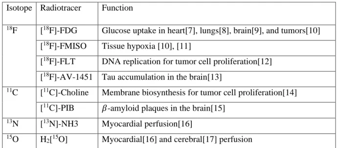
Table 1: Imaging of different physiological processes using different PET tracers ... 5

Table 2: Radiotracers for tau PET imaging ... 33

Table 3: ECAT HR+ parameters in 3D mashing mode ... 48

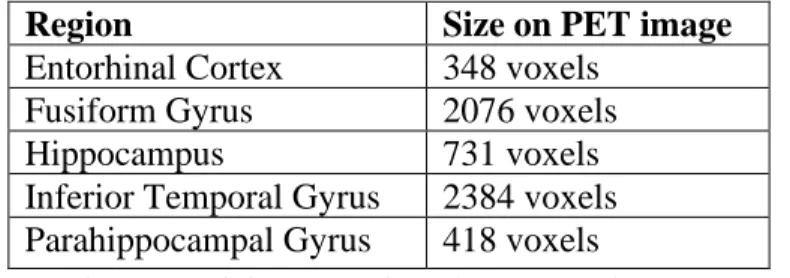
Table 4: The size of the considered ROIs on the PET image ... 51

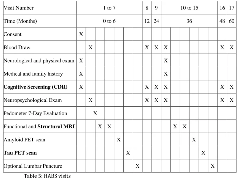
Table 5: HABS visits ... 55

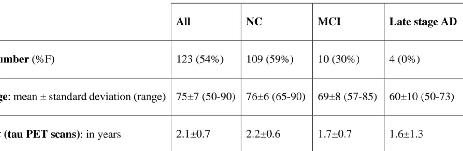
Table 6: Demographics. (%F) refers to the proportion of female subjects enrolled. 𝛥t refers to the time elapsed between the tau PET scans: mean ± t standard deviation. ... 56

Table 7: Sample sizes for the separation between groups with different tau accumulations using the two methods ... 93

LIST OF FIGURES

Figure 1: Schema of a PET scanner. It is composed of 4 block detector rings. The red line

shows two annihilations photons reaching two detector blocks in opposite sides. ... 7

Figure 2: Annihilation events: accepted (Blue) and rejected (Brown) by coincidence detection. ... 8

Figure 3: Scatter and random coincidences ... 9

Figure 4: 2D and 3D acquisition modes ... 10

Figure 5: Parametrization of a LOR... 10

Figure 6: Principle of iterative reconstruction algorithms ... 17

Figure 7: Hypothesized evolution of plaques and tangles in AD[72]. ... 30

Figure 8: Generation of a simulated PET data with an increased tau accumulation. (A) shows the background image: the PET image at 𝑡1. (B) represents the MR image and the segmentation label localizing the ITG after registration to the PET image. (C) is the obtained image after multiplying the mean value of SUV in ITG by a scaling factor. The image (C) is forward projected and a Poisson noise is added to get the sinogram (D). (E) is the initial PET data used to reconstruct the PET image. The summation of (E) and (D) yields the PET data for the simulated time-point 𝑡2. ... 53

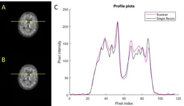
Figure 9: Comparison between the scanner and the implemented single time-point reconstruction. (A) is the image from the scanner with an overlaid line plot. (B) shows the same line plot on the reconstructed image using our OSEM implementation. (C) represents the profile plots along the line in (A) and (B). ... 63

Figure 10: The performance of the image registration. (A) shows the ITG and (B) shows the cerebellum cortex used as the reference region. Panel (1) presents the MR images with the overlaid masks from FreeSurfer segmentation. Panel (2) shows the same MR volumes after they were registered to the PET images. Panel (3) overlays the registered masks on the PET images. ... 64

Figure 11: Comparison between the background image (A) and the common image (B) obtained by the joint reconstruction, The profile plots in (C) of the line displayed in (A) and (B) show that the images are very similar. ... 65

Figure 12: The difference images for the simulated increase in tau accumulation. (A) shows the MR image with the ITG mask. Panel (B), in the top row, is composed of the difference images obtained by the joint reconstruction. Panel (C), in the bottom row, shows the difference images obtained by subtraction of the two images reconstructed separately. The level of the simulated increase in the tau deposition is also displayed. In panels (B) and (C), the PET images are shown with the colormap “hot” overlaid over the MR images (gray scale). ... 66

Figure 13: Sensitivity index in the difference images produced by the two methods as a function of the level of simulated increase in tau accumulation ... 67

Figure 14: Bias of the conventional and the proposed methods. ... 69 Figure 15: Standard deviation for the conventional and the proposed methods ... 69 Figure 16: Registration between the time-points. We show the PET images at 𝑡1 and 𝑡2 before (A) and after registration(B). The image at 𝑡1 is displayed with a gray scale. The image at 𝑡2 is displayed with the colormap “hot”. ... 71 Figure 17: Example of difference images for the 4 reconstruction methods. The rows show the images from a healthy subject, an MCI subject, and an AD subject. The images in the first three columns are obtained by the conventional method with an increasing number of included frames in the reconstruction. The last column shows the images of the joint reconstruction. The PET images are displayed with the colormap “hot” overlaid over the MR images (gray scale). ... 72 Figure 18: Regional variance averaged across all subjects obtained from the 4 difference images showing the voxel-wise change of SUVR between the two time-points. ... 73 Figure 19: Boxplot of 𝛥SUVR (expressed as a percentage of the SUVR in image at 𝑡1) in the ITG, computed for each subject, for each proposed method. ... 75 Figure 20: Boxplot of 𝛥SUVR (expressed as a percentage of the SUVR in image at 𝑡1) in the FG, computed for each subject, for each proposed method. ... 75 Figure 21: Boxplot of 𝛥SUVR in the ITG wherein only positive values are considered . 76 Figure 22: ROC for separability between NC and MCI ... 77 Figure 23: Change of SUVR between consecutive frames of the same scan of a healthy control subject ... 88 Figure 24: Average change of SUVR between consecutive frames expressed as the percentage of the SUVR in the previous frame ... 88 Figure 25: Phantom Simulations. (A) the simulated phantom (noiseless reference image) with the hippocampus mask in red. (B) the simulated image at 𝑡1 ... 90 Figure 26: Difference image for a tau accumulation increase of 10%. (A) Conventional method. (B) Proposed method. The red arrows point to the signal detected in the hippocampus region. ... 91 Figure 27: ROC for the separability between the groups with 7% and 5% increase in tau accumulation ... 93 Figure 28: Bias-Variance plot for the joint reconstruction with two different priors compared to the conventional method. ... 94

LIST OF SYMBOLS AND ABBREVIATIONS

AD Alzheimer’s Disease

PET Positron Emission Tomography

SPECT Single Photon Emission Computed Tomography MR Magnetic Resonance

LOR Line of Response

MLEM Maximum Likelihood Expectation-Maximization OSEM Ordered Subsets Expectation Maximization

SUV Standard Uptake Value SUVR Standard Uptake Value Ratio

PHF Paired Helical Filament ROI Region Of Interest

EC Entorhinal Cortex FG Fusiform Gyrus HC Hippocampus

ITG Inferior Temporal Gyrus PHG ParaHippocampal Gyrus

STIR Software for Tomographic Image Reconstruction HABS Harvard Aging Brain Study

CDR Clinical Dementia Rating MMSE Mini Mental State Exam

NC Normal Control

SUMMARY

The accumulation of the paired helical filament tau protein leads to the cognitive decline seen in Alzheimer’s disease (AD). The Positron Emission Tomography tracer, [18 F]-AV-1451, permits the observation of PHF tau in vivo. To determine the rate of tau deposition in the brain, the conventional approach involves scanning the subject two times (2-3 years apart) and reconstructing the images separately. Region-specific rates of accumulation are derived from the difference image which suffers from an increased intensity variation making this approach inadequate for clinical trial looking at the effect of a candidate drug on tau because the increased variation leads to a higher sample size required.

We propose a joint longitudinal image reconstruction where the tau deposition difference image is reconstructed directly from measurements leading to a lower intensity variation. This approach introduces a linear temporal dependency and accounts for spatial alignment, and the different injected doses.

We validate the reconstruction method by simulating higher tau accumulation in real data at different intensity levels. We additionally reconstruct the data from 123 subjects: 109 healthy subjects, 10 suffering from mild cognitive impairment, and 4 diagnosed with AD.

The joint reconstruction shows better contrast in the difference image obtained by the numerical simulations and a drastically reduced variance in the change of the Standard Uptake Value Ratio (SUVR) among subjects.

Introduction

Positron Emission Tomography (PET) is a functional, nuclear imaging modality that has become an integral part of patient management in a clinical setting. Nuclear imaging permits the observation of a physiological process as opposed to anatomical imaging which show the structures inside the body. As we explain in Chapter 1, PET enables the imaging of the spatiotemporal distribution of a radiotracer injected in the patient’s body. As the attached radionuclide undergoes a radioactive decay, a positron is emitted and eventually encounters an electron leading to the production of two annihilations 511 keV photons that are detected by the PET camera. Reconstruction algorithms, incorporating data correction factors, produce a quantitative image reflecting the distribution of the radiotracer which has been designed to target a specific process in the body. The multitude of radiotracers available explains the broad use of PET imaging in the clinic and research settings. In this work, we focus on one recently developed radiotracer: [18F]-AV-1451 which permits the observation of the distribution of Paired Helical Filament (PHF) tau protein in the brain.

The appearance of excessive amounts of the PHF tau protein has been linked to the process of cognitive decline seen in dementia caused by Alzheimer’s disease (AD). AD is an irreversible chronic neurodegenerative disease, the most common cause of dementia among the elderly. It is one of the biggest health problems facing our society. The cost of caring for AD patients is around $290 billion per year in the United States alone and is expected to increase as the population ages[1]. In Chapter 2, we give a brief presentation of AD and the role of tau protein in the disease. Recent histopathological and tau PET studies (using [18F] AV-1451) suggest that prodromal AD may be monitored by following

the spread of PHF tau in the entorhinal cortex (EC), parahippocampal gyrus (PHG), fusiform gyrus (FG), inferior temporal gyrus (ITG), and the hippocampus (HC). We mainly focus on the role of PET imaging to accurately estimate the changes in tau protein deposition in the brain of subjects undergoing longitudinal studies.

The aim of this work, as presented in Chapter 3, is the development of a PET reconstruction framework enabling the estimation of tau deposition rate directly from two longitudinal [18F] AV-1451 scans to improve the accuracy of diagnosis in early stages of AD and aid the development of treatments that halt its advancement. As we explain in

Chapter 4, the proposed joint reconstruction framework for longitudinal studies results in

a reduction in the variance of the estimated difference image as compared to the one produced using the conventional method consisting in taking the difference between images reconstructed separately. In Chapters 5 and 6, we apply our joint framework to simulations and to longitudinal patient studies. The validation of the joint method is discussed in Chapter 7, first by comparing the images obtained after considering a single scan from a patient study to the clinical image; second, by evaluating the results on the simulations. In Chapter 8, we present the results applied to the patient cohort and use them to derive sample sizes for both methods for a hypothetical clinical trial aiming at separating between groups exhibiting different rates of tau accumulation. Finally, in Chapter 9, we discuss the limitations of the proposed approach and provide an alternative formulation for the reconstruction problem using temporal priors.

CHAPTER 1.

Positron Emission Tomography

Positron Emission Tomography (PET) is a powerful imaging technique that provides quantitative evaluation of imaged tissues. It has been reported as the most specific and sensitive technique for in vivo imaging of molecular interactions[2] as its performance exceeds by far that of Single Photon Emission Computed Tomography (SPECT)[3]. The quantitative information inferred from PET images enables a fast and reliable assessment of various conditions, leading to the prevalence of PET imaging in clinical applications[4]. In this chapter, we discuss the physical foundations[5], [6] of PET imaging from the radioactive decay to the photon detection in the scanner. The measurements are then converted to PET data that are reconstructed into images after applying several corrections techniques.

1.1 Physical Foundations

A PET study begins by the injection of a radioactive tracer in the patient’s body. Different tracers can be used depending on the purpose of the study. The process of radioactive decay leads to positron emission inside the patient’s body. As a positron encounters an electron, annihilation occurs, which leads to the emission of two 511 keV photons travelling in almost opposite directions. The PET scanner detects photon pairs and backtracks their paths to localize the annihilation points, thereby generating a map of the distribution of the radiotracer: a PET image.

1.1.1 Radiotracers

The radiotracer is a compound formed by attaching a radionuclide to a molecule to enable the tracking of said molecule inside the patient’s body. Two important principles govern the radiotracer design: it is assumed to behave the same way as the original molecule or at least in a known and predictable matter, and its mass and/or concentration should not interfere with the physiologic process that is being imaged.

Fluorine 18 (18F) is widely used as the labelling radionuclide in PET imaging: its half-life of 109 minutes is long enough to perform an imaging study and short enough to limit the radiation exposure. The most used radiotracer is fluorodeoxyglucose [18F]-FDG which is a marker for tissue uptake of glucose and has become indispensable in oncology. Table 1 below presents examples of radiotracer and the corresponding physiological processes they target.

Isotope Radiotracer Function

18_{F [}18_{F]-FDG Glucose uptake in heart[7], lungs[8], brain[9], and tumors[10]}

[18_{F]-FMISO Tissue hypoxia [10], [11]}

[18F]-FLT DNA replication for tumor cell proliferation[12] [18F]-AV-1451 Tau accumulation in the brain[13]

11_{C [}11_{C]-Choline Membrane biosynthesis for tumor cell proliferation[14]}

[11C]-PIB 𝛽-amyloid plaques in the brain[15]

13_{N [}13_{N]-NH3 Myocardial perfusion[16]} 15_{O H}

2[15O] Myocardial[16] and cerebral[17] perfusion

1.1.2 Radioactive decay and interactions

A positron emitting radionuclide (𝐴_𝑍𝑋) decays to a stable nucleus (_𝑍−1𝐴𝑌) by emitting a positron (𝑒+_{) and an electron neutrino (𝜈}

𝑒):

𝑋 = _𝑍−1𝐴𝑌

𝑍

𝐴 _{+ 𝑒}+_{+ 𝜈} 𝑒

For example, 18F, with 9 protons and 9 neutrons, decays to 18O which a stable isotope of oxygen with 8 protons and 10 neutrons, by emitting a positron.

The positron and the neutrino are ejected with the kinetic energy produced by the decay. The positron loses its energy after few collisions with its surrounding atoms. Once it slows down, it annihilates with an electron. The rest energy of both the positron and the electron is 511 keV. The annihilation leads to the appearance of two 511 keV photons that are travelling in almost opposite directions.

In practice, the positron is not fully stopped when it interacts with the electron. As a result, the photons are not perfectly collinear: they form an angle deviating from the theoretical 180° by a few tenths of a degree. Since PET imaging relies on the photons path to recover the location of the annihilation event, the non-collinearity of the photons limits the spatial resolution of the PET system. Furthermore, the distance travelled by the positron before annihilation occurred – called the positron range – introduces uncertainty about the real spatial distribution of the radiotracer: the image reflects the location of the annihilation event, not the location where the radioactive decay occurred. In the case of the 18F tracer, the positron range is estimated between 0.6 mm and 2.4 mm in water[18], and the angle between the annihilation photons ranges from 179.75° and 180.25°[19].

As the emitted photons travel through the matter, they undergo two types of interactions that are important in PET imaging:

• Photoelectric effect: the photon is absorbed by an atom and an electron is emitted. • Compton scattering: the photon is deflected after it collides with an electron in the outer shell of an atom. It loses some of its energy, but it is not completely absorbed by the atom as in the photoelectric effect. The angle between the incident photon and the deflected one can vary from 0 to 180°[20].

As a result, the photons detected by the PET scanner may display a different energy and a different direction from what is expected after an annihilation. These are known as scattered events.

1.1.3 Coincidence detection

A PET scanner contains blocks of photons detectors arranged in concentric rings around the object to be imaged. Figure 1 shows the configuration of a scanner with 4 block detector rings where two annihilation photons reach two detector blocks in opposite sides.

Most detectors in commercial scanners are inorganic scintillation detectors[21] whose role is to absorb the incident photon and convert it to many visible light photons. A photomultiplier tube detects these photons and produces a proportional electric signal that contains information about the time when the incident photon was

Figure 1: Schema of a PET scanner. It is composed of 4 block detector rings. The red line shows two annihilations photons reaching two detector blocks in opposite sides.

detected, as well as its energy. A pulse-height analysis is then performed to record annihilation events: only a pair of collinear photons each at 511 keV arriving to the detectors at the same time constitute a counted event. In practice, a temporal window, around 10 ns[6], defines the accepted delay between the photons and an energy window, generally set to (440 keV, 650 keV)[6], defines the accepted deviation from the ideal 511 keV level for the detected photons.

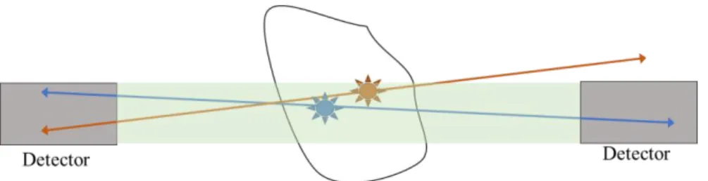
Figure 2: Annihilation events: accepted (Blue) and rejected (Brown) by coincidence detection.

Figure 2 shows an example of an annihilation event (in blue) that has been counted by a pair of the detectors, if the photons arrive within the temporal window and with an accepted energy. The annihilation event in brown is not counted for the shown pair of detectors as one of the resulting photons is outside of the green area, which represents a 3D tube linking the two detectors, and therefore it is not detected. Every time an annihilation event occurs in that tube – if the resulting photons remain inside the tube, the number of events recorded for that pair of detectors is incremented. The 3D tube between the two detectors is commonly called the Line of Response (LOR).

Based on their detected positions, their energies, and the times of the detection, some photons resulting from annihilation events are discarded. The opposite can also occur: the scanner incorrectly records events known as random coincidences. In Figure 3, the scanner increments the count of the LOR shown by

the dashed lines leading to incorrect positioning of the true annihilation events[5]:

• Scatter coincidence occurs when one photon is scattered and is therefore recorded in a detector different from the one that would be involved in the true LOR. Even if the scattered photon ends up hitting the detector with a small delay compared to the other photon involved in the annihilation event, the time difference is usually smaller that the temporal window.

• Random coincidence occurs when two annihilation events are mistakenly recorded as one. For example, if two photons from two unrelated annihilation events get absorbed in the imaged body and the two remaining photons hit a pair of opposing detectors within the temporal window, then the scanner will increment the counted events for that LOR although no annihilation occurred along that line.

The process of coincidence detection sometimes rejects true events and counts false ones. This contributes to the loss of contrast in the PET images. However, there are techniques to correct for some of these effects (Section 1.2).

1.1.4 Data formation

PET data acquisition can be performed in 2D or 3D modes, as shown in Figure 4. In 2D PET mode, lead septa are used to only allow the detection of coincidences in the same ring or in adjacent rings. This acquisition scheme leads to a reduction in accidental coincidences but also a reduction in the scanner sensitivity. The septa are

removed in 3D mode so that coincidence from different planes can be detected[6].

2D PET imaging sees the volume as transverse slices along the z axis. The LOR contained inside the specified plane is parametrized with an angle

𝜙 and its distance from the center 𝑠 as shown in Figure 5. For a given plane 𝑧 and a given direction 𝜙, the LORs are defined by their distances from the center. Each is assigned the number of annihilation events counted by the pair of the detectors. The set of LORs for varying directions and distances from the center is called a sinogram. Once the events along the LORs from all the slices forming the volume have been counted, we obtain

a three-dimensional table composed by the superposition of sinograms from different planes.

Figure 4: 2D and 3D acquisition modes

The LORs composed by a pair of detectors in the same ring are called “direct”. Oblique planes link detectors from different rings as illustrated in Figure 4 and yield “indirect” LORs which are also organized in sinograms.

The PET data collected by the scanner is a matrix indexing every possible LOR and saves its assigned count reflecting the distribution of the radiotracer along that LOR. Image reconstruction algorithms transforms these measurements into a 3D image. However, some correction techniques should be applied to yield a quantitative image.

1.2 Corrections toward quantitative PET

To ensure that the reconstructed image truly reflects the underlying function, correcting for physical phenomena negatively affecting the detections is necessary. We have already discussed sources of errors in PET imaging resulting from the positrons and the photons interactions in the imaged object. We will describe how we can correct their effects when possible.

1.2.1 Random coincidences correction

Random coincidences occur when two unrelated annihilation events lead to two detected photons within the temporal window as shown in Figure 3. Their spatial distribution is uniform across the field of view and is nearly independent from the imaged object, as opposed to true coincidence which reflect the distribution of the radiotracer. Therefore, the fraction of random detections is higher for regions where true coincidences are highly attenuated and can lead to more pronounced quantitative errors in these regions.

• Single rates: The rate 𝐶_𝑖𝑗 of random coincidences in a specified LOR (𝑖, 𝑗) is a function of the temporal window length (2𝜏) and the rate of single counts in the detectors 𝑖 and 𝑗 forming that LOR[22], noted 𝑟𝑖 and 𝑟𝑗: 𝐶𝑖𝑗 = 2𝜏𝑟𝑖𝑟𝑗. The total

number of random coincidences in that LOR is then estimated over the acquisition time 𝑇 if the radiotracer redistribution is ignored[23]: 𝑅𝑖𝑗 =

2𝜏

𝑇 𝑅𝑖𝑅𝑗 where 𝑅𝑖 is the

total number of single photons counted in the detector 𝑖.

• Delayed coincidence channel[22]: the temporal window is delayed by a duration equal to many times its width so that the coincidences in the delayed window cannot arise from the same annihilation event or scattered photons. The counts detected in the delayed window is a direct measure of the number of random coincidences and are assumed to be the same in original temporal window as coincidences in both windows are subject to the same counting limitations.

The delayed coincidence channel is the most commonly implemented technique[24] as it is the most accurate. However, it propagates the noise of the estimated random coincidences directly into the corrected data.

1.2.2 Compton scatter correction

As photons travel through matter following annihilation events, they can be deflected from their original trajectory when they undergo a Compton scatter interaction. As a result, the annihilation event will be assigned to the wrong LOR (Figure 3). Scatter coincidences will induce large quantification errors if left uncorrected as they represent a large fraction of the measured coincidences.

Analytical estimation of the scatter is possible under the assumption that only one of the annihilation photons is scattered once. In that case, the following formula[25] gives the single scatter coincidence rate in the LOR of the detectors 𝑖 and 𝑗:

𝐷_𝑖𝑗 = ∫ [ 𝜎𝑖𝑃𝜎𝑗𝑃 4𝜋𝑑_𝑖𝑃2 𝑑_𝑗𝑃2 𝜇 𝜎𝑐 𝑑𝜎𝐶 𝑑Ω (𝐼𝑖+ 𝐼𝑗)] 𝑉 𝑑𝑉

• 𝑃 is a moving point in the integration volume (noted 𝑉) where the Compton scattering occurs.

• 𝜎_𝑖𝑃 is the cross section of the detector 𝑖 as seen from the point 𝑃. • 𝑑_𝑖𝑝is the distance between the detector 𝑖 and the scattering point 𝑃. • 𝜇 is the attenuation coefficient in the point 𝑃.

• 𝑑𝜎𝑐

𝑑Ω is the differential Compton scattering cross-section derived from the

Klein-Nishina formula.

• 𝐼_𝑖 calculated the intensities of the attenuated photons if the scattered photon arrives on the detector 𝑗. The opposite case, where the scattered photon reaches the detector 𝑖, is accounted for in the twin term 𝐼_𝑗.

The analytical estimation of the scatter is computationally expensive; thus, it is only performed in a reduced number of points picked randomly in the attenuation volume. It also requires the prior knowledge of the activity distribution: an iterative scheme is thus needed. First, the activity distribution is estimated without the scatter correction, then, the scatter is estimated using the analytical calculation. Finally, the scatter correction can be incorporated into the estimation of the activity distribution.

The analytical solution for scatter estimation is fast and noise free. However, it only accounts for single scatter events. This assumption is reasonable as a single scatter occurs in 75% to 80% of all scattering events in a ring of 10 cm axial field of view[26]. This means that the solution underestimates scatter by around 20%. Instead of modeling multiple scattering events or performing Monte Carlo calculations, it is possible to scale the obtained scatter sinogram to account for all scattering events. All the events detected

outside of the subject are due to Compton scattering. The ratio between these events and the simulated single scatter outside of the subject thus provides the scaling factor between the multiple scatter events and the single ones. It is therefore applied to the obtained single scatter sinogram to obtain an accurate estimation of all scattering events.

1.2.3 Attenuation correction

Attenuation correction aims to correct for photons that should have been detected but they were not either because they were completely absorbed or because their energy/direction following different interactions led the detection analyses to discard them.

In PET, the attenuation of the annihilation photons is independent of the position of the annihilation event along the LOR: for a homogenous object, the probability of detecting the pair of the photons is 𝑝 = exp (−μT) where 𝑇 is the thickness of the object, and 𝜇 is the linear attenuation coefficient of the tissue comprising the imaged object at 511 keV. The attenuation coefficient is around 0.095 cm−1 for soft tissue, between 0.12 and 0.14 cm−1 _{for bone, and around 0.04 cm}−1 _{in the lungs[6].}

Attenuation correction techniques rely on the estimation of the attenuation along all the LORs. It can be done by comparing the count rate from an external transmission source (transmission scan) with the count rate from the same source without the subject (blank scan). The ratio between the counts of transmission scan and those of the blank scan yields an estimation of the probability that the photons are not absorbed in each LOR: exp (− ∫_𝐿𝑂𝑅𝜇(𝑙)𝑑𝑙) [5].

Nowadays, most commercial PET scanners are combined systems incorporating both PET and CT imaging[27]. A CT scan measures the attenuation of photons after they travel through the patient body along each LOR. This is the measure we are trying to estimate to correct for photons attenuation in the PET image. An empirical bilinear function[28] permits the conversion of the attenuation coefficients measured by the CT scan to their equivalent at the PET energy level (511 keV).

1.2.4 Detector normalization

A PET scanner houses thousands of individual detectors. Inevitably, they will display variations in their performance[6]: some are due to intrinsic factors (crystal imperfections, difference in PMT gains, variation in the electronics used to detect signal…), others are geometric (the position of the detector in the ring/block , the incidence angle of the detected photon…). These variations are linked to the scanner itself and are independent of the imaged object. Correction for these effects is called normalization.

If all the detectors are exposed to the same radiation source, the difference in detected counts reflects directly the variation across the detectors. The blank scan used to derive the attenuation probability across LOR accomplishes the same outcome: all detector pairs receive the same number of annihilation photons after one revolution of the external source around the field of view. A noisy estimation of the normalization factors will affect the noise levels in the true coincidences counts. To diminish the noise in the normalization correction, a long acquisition is needed which is not always feasible. Instead, the factors are decomposed into many components each reflecting one source of variation. The estimation of these new factors can be done using simple phantoms, low activity levels,

and long acquisitions as they are dependent on the scanner and don’t need to be repeated for each scan[29].

1.3 Tomographic Image Reconstruction

We have seen in Section 1.1.4 how the scanner saves the acquisition data in a matrix where each element represents one LOR and stores its corresponding count. Many factors undermine the accuracy of the recorded counts and correction techniques need to be implemented to get reliable data (Section 1.2). The next step consists in transforming the count data to a 3D image representing the distribution of the radiotracer in the imaged object. The transformation is known as tomographic image reconstruction.

Two types of algorithms are applied to the PET image reconstruction: the analytical methods which are based on an over-simplified model of the measured data and the iterative methods which use a more accurate model of the physical effects involved in PET imaging. In the following section, we present the widely used iterative reconstruction algorithm: Ordered Subsets Expectation Maximization (OSEM)[30].

1.3.1 Iterative reconstruction

The general concept of an iterative reconstruction algorithm is shown in Figure 6: the imaged object is approached by successive estimates, iteratively updated using the difference between the calculated projections from the preceding iteration and the real measured projections. The approximation is repeated until the difference between the measured data and the calculated projections is minimal. The latest estimate gives the reconstructed image.

From Figure 6, we can identify the five ingredients on an iterative reconstruction algorithm, the data model (the representation of the measured projections), the image model (based on the discretization of the field of view in contiguous and non-overlapping voxels), the system matrix (the link between the image model and the data model), the cost function (the comparison between the measured and the calculated projections), and the optimization algorithm (the definition of the update step in each iteration).

Figure 6: Principle of iterative reconstruction algorithms

To simplify the representation of the data, a single index 𝑗 is used to define the LOR between two detectors (𝑘,𝑙). 𝑛_𝑗 denotes the number of events detected for the LOR 𝑗. The PET data is the result of photons annihilation following the emission of a positron in the radioactive decay process. Therefore, the 𝑛_𝑗 are distributed as independent Poisson variables[5]. The likelihood function defined as the probability of measuring the counts 𝑛_𝑗 as a function of the parameter to estimate (here, the image 𝝀) is given by:

𝐿(𝝀|𝒏) = ∏𝑒𝑥𝑝(−𝑝𝑗) 𝑝𝑗 𝑛𝑗 𝑛_𝑗! 𝐾 𝑗=1 (1)

where 𝐾 is the total number of LORs, and 𝑝_𝑗 is the expected value of the counts detected for the LOR 𝑗.

Likewise, the image 𝝀 is represented as a column vector of activity values in its voxels. Let’s note 𝑀 the number of the voxels in the image. The discretized problem is then composed of linear equations:

𝑝𝑗 = ∑ ℎ𝑗,𝑖𝜆𝑖 𝑀 𝑖=1

(2)

The elements ℎ_𝑗,𝑖 express the probability of detecting a primary emission from the voxel 𝑖 in the LOR 𝑗. The system matrix 𝑯, composed of the elements ℎ_𝑗,𝑖, has the size 𝑲 × 𝑴. The vector form of the reconstruction problem is written: 𝒑 = 𝑯𝝀, where 𝒑 is a column vector 𝒑 = 𝒏̅.

In iterative reconstruction algorithms, a current image is fed to the system matrix yielding calculated projection data (Figure 6) that can be compared to the measured data. This comparison is enabled by the cost function. In the OSEM algorithm, the cost function is defined as the natural logarithm of the likelihood 𝐿(𝝀|𝒏) in Equation (1):

ln(𝐿(𝝀|𝒏)) = ∑ −𝑝_𝑗

𝐾 𝑗=1

+ 𝑛_𝑗ln (𝑝_𝑗) − ln 𝑛_𝑗! (3) Incorporating the forward model in Equation (2), we obtain:

ln(𝐿(𝝀|𝒏)) = ∑ (− ∑ ℎ_𝑗,𝑖𝜆_𝑖 𝑀 𝑖=1 + 𝑛_𝑗ln (∑ ℎ_𝑗,𝑖𝜆_𝑖 𝑀 𝑖=1 ) − ln 𝑛_𝑗!) 𝐾 𝑗=1 (4)

The reconstructed image estimate is given by:

𝝀̂ = argmax

𝝀 (ln(𝐿(𝝀|𝒏))) (5)

If we ignore the terms that are independent from 𝝀, we finally obtain:

𝝀̂ = argmax 𝛌 (∑ (− ∑ ℎ𝑗,𝑖𝜆𝑖 𝑀 𝑖=1 + 𝑛_𝑗𝑙𝑛 (∑ ℎ_𝑗,𝑖𝜆_𝑖 𝑀 𝑖=1 )) 𝐾 𝑗=1 ) (6)

The optimization algorithm solves the problem defined in Equation (6) and yields the current estimated image.

To derive the Expectation-Maximization (EM) algorithm[31] used in OSEM, we need to look at the complete data: the measured data 𝒏 is incomplete because it only gives the number of counts in LORs, but we ignore what fraction of these counts originated from a specific voxel. The complete data is defined as the number of counts detected in a LOR 𝑗 and originated from the voxel 𝑖 and it is noted 𝑁_𝑗,𝑖. The maximum likelihood for the complete data is given by:

𝐿(𝝀|𝑵) = ∏ ∏exp(−𝑝𝑗,𝑖) 𝑝𝑗,𝑖 𝑁𝑗,𝑖 𝑁𝑗,𝑖! 𝑀 𝑖=1 𝐾 𝑗=1 (7)

where 𝑝_𝑗,𝑖 is the mean value of the counts in the LOR 𝑗 that came from the voxel 𝑖. As we have previously stated, the probability of detecting an event in the LOR 𝑗 originating in the

voxel 𝑖 is given by the element ℎ_𝑗,𝑖 of the system matrix. We have then: 𝑝_𝑗,𝑖 = ℎ_𝑗,𝑖𝜆_𝑖. Finally, the log-likelihood for the complete data, noted 𝑙(𝝀|𝒏), is given by:

𝑙(𝝀|𝒏) = ∑ ∑ −ℎ_𝑗,𝑖𝜆_𝑖 𝑀 𝑖=1 + 𝑁_𝑗,𝑖ln(ℎ_𝑗,𝑖𝜆_𝑖) − ln(𝑁_𝑗,𝑖!) 𝐾 𝑗=1 (8)

In the EM algorithm, instead of maximizing the log-likelihood directly, we want to maximize its mean value. If we note 𝝀𝑘 the estimated image at the iteration 𝑘 of the optimization algorithm, then the expectation step of the EM gives:

𝔼[𝑙(𝝀|𝒏)| 𝒏, 𝝀(𝒌)] = ∑ ∑ −ℎ𝑗,𝑖𝜆𝑖 𝑀 𝑖=1 + 𝔼[𝑁𝑗,𝑖|𝒏, 𝝀(𝒌)] 𝑙𝑛(ℎ𝑗,𝑖𝜆𝑖) − 𝔼 [𝑙𝑛(𝑁𝑗,𝑖!)| 𝒏, 𝝀(𝒌)] 𝐾 𝑗=1 (9)

The 𝑁_𝑗,𝑖 are Poisson distributed so the conditional probability distribution given their sum (since 𝑛_𝑗 = ∑𝑀_𝑖=1𝑁_𝑗,𝑖) is a binomial distribution with parameters (𝑛_𝑗, ℎ𝑗,𝑖𝜆𝑖

∑𝑀𝑞=1ℎ𝑗,𝑞𝜆𝑞).

Therefore, the expectation of the complete data given their sum and the current image is:

𝔼[𝑁𝑗,𝑖|𝒏, 𝝀(𝑘)] = 𝑛𝑗

ℎ_𝑗,𝑖𝜆_𝑖(𝑘)

∑𝑀_𝑞=1ℎ_𝑗,𝑞𝜆(𝑘)_𝑞 (10)

We can ignore the last term in Equation (9) because it will be set to zero in the maximization step as it is independent of 𝝀.

The maximization step consists in differentiating the Equation (9) with respect to a voxel 𝜆_𝑙 and setting the derivative to zero. Finally, we obtain the update formula:

𝜆_𝑙(𝑘+1) = 𝜆𝑙 (𝑘) ∑𝐾_𝑗=1ℎ_𝑗,𝑙∑ ℎ_𝑗,𝑙𝑛_𝑗 ∑ ℎ𝑗,𝑞𝜆𝑞 (𝑘) 𝑀 𝑞=1 𝐾 𝑗=1 (11)

The Maximum Likelihood Expectation Maximization (MLEM) algorithm in Equation (11) is guaranteed to converge and it is unbiased[32]. However, it may require many iterations to reach convergence. The resulting image, after many iterations, is then too noisy to be useful in practice. To minimize the noise level in the reconstructed image, the process is stopped before reaching convergence and therefore bias is introduced in the final image. Around 100 iterations are still needed to get a reasonable solution. OSEM has been introduced to speed up the convergence: for every iteration, the measurements 𝒏 are separated into subsets and the update step of the MLEM algorithm is applied multiple times, each time using the data from a single subset. This technique is widely used in clinical applications because it yields images like the MLEM’s solution with a decreased reconstruction time. However, OSEM does not converge to the maximum-likelihood solution because not all the data is used for each update step[33].

We have derived the MLEM algorithm as an example of an iterative reconstruction algorithm. We have explained how it can be modified to get the widely used OSEM version. The question that we try to answer next is how to incorporate the data correction techniques seen in Section 1.2 in the reconstruction framework.

1.3.2 Corrected PET data reconstruction

We have previously introduced the elements of the system matrix 𝑯 as the probability for a positron emitted in voxel 𝑖 to be detected without scattering in LOR 𝑗. The matrix 𝐻 can, in fact, be decomposed in a product of matrices, each modeling one phenomenon of the

acquisition scheme: 𝑯 = 𝑺𝑨𝑮. 𝑮 incorporates the geometry of the scanner and gives the geometric probability of detecting an annihilation event from the voxel 𝑖 in the LOR 𝑗. 𝑮 has the same size as the system matrix 𝑯. 𝑺 and 𝑨 are diagonal matrices of size 𝐾 × 𝐾 containing the sensitivity (Section 1.2.4) of the LORs and their attenuation factors (Section 1.2.3), respectively.

The effect of the scattered and the random coincidence is seen directly in the measurements: 𝒏 = 𝒕 + 𝒅 + 𝒓, where 𝒕 reflects the number of true coincidences counted in each LOR, 𝒅 is the number of scattered coincidences, and 𝒓 is the number of random coincidences. 𝑡_𝑗,𝑑_𝑗, and 𝑟_𝑗 are Poisson distributed, their sum is also Poisson. The mean of the 𝑡_𝑗, true coincidences in the LOR 𝑗, is 𝑝_𝑗 as described in Equation (2). Let’s note 𝑑̅ and _𝑗 𝑟𝑗

̅ the mean values of 𝑑𝑗 and 𝑟𝑗. Then: 𝔼[𝑛𝑗] = ∑𝑀𝑖=1ℎ𝑗,𝑖𝜆𝑖 + 𝑑̅ + 𝑟𝑗 ̅. Additionally, the 𝑗

elements of the system matrix are rewritten as ℎ_𝑗,𝑖= 𝑎_𝑗𝑠_𝑗𝑔_𝑗,𝑖 to show the contribution of the attenuation coefficients and the normalization factor. We can finally follow the same steps performed in Section 1.3.1 to rewrite the problem for the EM algorithm and obtain the following update step[31]:

𝜆_𝑙(𝑘+1) = 𝜆𝑙 (𝑘) ∑𝐾 𝑎_𝑗𝑠_𝑗𝑔_𝑗,𝑙 𝑗=1 ∑ 𝑎𝑗𝑠𝑗𝑔𝑗,𝑙𝑛𝑗 ∑𝑀_𝑞=1𝑎_𝑗𝑠_𝑗𝑔_𝑗,𝑞𝜆(𝑘)_𝑞 + 𝑑̅ + 𝑟_𝑗 ̅_𝑗 𝐾 𝑗=1 (12)

With the incorporated PET data corrections, the reconstruction algorithm yields a quantitative PET image which can be analyzed in a clinical setting.

1.4 Clinical applications of PET

The multitude of radiotracers and their different functions illustrated in Table 1 explains how prevalent PET imaging in patient management is. We focus on three main areas in this section.

1.4.1 Oncology

PET imaging serves primarily as a diagnostic tool in oncology. The widely used [18_F]-FDG

tracer enables the imaging of glucose uptake in the body. Since most cancerous cells are glucose avid, the resulting PET images show an increased uptake where tumors are located[34]. This ability makes PET imaging valuable not only for diagnoses but also for patient management throughout their care as it can detect residual disease post-treatment. It is an integral part of the patient follow-up owing to its ability to distinguish between post-treatment scarring and active tumor recurrence[35].

Tumor detection and post-treatment imaging usually relies on a qualitative interpretation of the image. In oncology, a semi-quantitative metric has been introduced: Standard Uptake Value (SUV) is derived from the image and it reflects how much of the injected activity is concentrated in that region and/or voxel; it plays a major role in therapy assessment[36]. Tracking the change of the SUV following treatment helps determine how well the patient is responding to therapy and if a change of his/her course of treatment is needed.

Additionally, [18F]-FDG PET imaging is present in radiation oncology. The therapy consists in defining the volume around the tumor and irradiating it. It is necessary to cover the whole volume where tumor cells are present for better outcome. It can be beneficial to

incorporate functional imaging in the definition of the contours of the regions to be targeted by radiation[37].

Finally, other radiotracers should be mentioned in cancer management: [18F]-FMISO which detects hypoxia in tumors to inform about their potential resistance to treatment[10], [11C]-Choline [14] and [18F]-FLT which are both markers for tumor proliferation [12] and are used in patient follow-up.

1.4.2 Cardiology

PET imaging enables the measurements of myocardial perfusion using the tracer [13

N]-NH3 and myocardial viability using the tracer [18F]-FDG. The former permits the comprehensive evaluation of the hemodynamic consequences of coronary artery disease (CAD) even before it becomes symptomatic, thus giving subjects with low cardiovascular risk earlier access to preventive therapy[38]. It is possible to monitor patients’ response to therapy or lifestyle changes thanks to the quantitative measure of myocardial perfusion. [18F]-FDG PET has also a high diagnostic value in assessing the myocardial viability of subjects with known CAD[7]. This assessment is very important considering that it is closely related to the risks and benefits of medical treatments and/or revascularization.

1.4.3 Neurology

PET imaging of the brain encompasses many areas. Naturally, one of the most prevalent uses is the diagnostic and management of brain cancers. As with most tumors, an increased [18F]-FDG uptake is indicative of cancer in the brain. [18F]-FDG is not the only tracer used in brain cancer: [18F]-FMISO, H2[15O], and [18F]-FLT have been used to assess hypoxia,

perfusion, and proliferation (respectively) in tumors[39], [40]. In the case of gliomas, [18

F]-FDG PET imaging findings have been linked to the tumor grade and the survival rates[41]. In epilepsy, it permits the localization of the seizure focus[42] needed in the case of required surgical therapy[43].

In addition, [18F]-FDG PET is a biomarker for neuronal degeneration in dementia[44]: its spatial distribution enables clinicians to make early diagnosis and to distinguish between different subtypes of dementia[45]. Many other tracers have been developed for PET imaging in dementia. In the next chapter, we study their use to image tau protein in relation to AD.

CHAPTER 2.

Tau Protein in Alzheimer’s Disease

Alzheimer narrated his discovery of a new disease[46] after observing one patient in a mental health facility. He described her rapid memory loss and her spatial and temporal confusion. He noted a rapid decline in her cognition and behavior. She was believed to be delusional and incoherent in her answers and actions. Her case was unusual because of her young age: her ordeal started in her early fifties. Upon her death, Alzheimer performed an autopsy on her brain and discovered a general atrophy of the brain and noted the presence of fibrils inside of normal-appearance cells and the deposition of a substance in the cortex: Alzheimer was then describing the tangles (tau protein) and the plaques (amyloid protein) that define AD. In this chapter, we give a brief introduction of the disease and we focus on PET imaging of tau protein.

2.1 Alzheimer’s disease

AD is an irreversible neurodegenerative disease and the most common cause of dementia among the elderly. Its symptoms consist in memory loss, language impairment, and a loss in the ability to recognize objects and/or people.

Age[47] is the most important risk factor for developing AD but there are many others such as environmental and genetic factors.

AD is characterized by the presence of two abnormal structures in histopathology studies: plaques (deposits of amyloid protein) and tangles (deposits of tau protein).

The disease progression can be separated in three phases[48]: pre-clinical, mild cognitive impairment (MCI) due to AD, and dementia. The first phase can last up to decades and reflects the long and slow formation of tangles and plaques seen in AD but without the manifestation of any cognitive decline. The second phase corresponds to the appearance of the first clinical signs of AD; however, the tentative diagnosis is made in accordance to other biomarkers and imaging techniques and by eliminating other causes of clinical signs. Finally, the last stage is Alzheimer’s dementia.

AD is a neurodegenerative disease characterized by a rapid decline in cognition: memory loss is the main feature of the disease. The episodic memory is related to personal events and experiences that are stored in the hippocampus[49], the first region to suffer damage in AD[50]. Therefore, the affected individual first forgets details about their own experiences. Semantic memory[49] loss occurs next: one forgets the general concepts of knowledge leading to language impairment[51] when the patient cannot recall the correct words. The inability to perform some tasks because of motor disorder as opposed to not understanding the tasks, also known as apraxia, is another sign of AD that can be present independently from memory loss[52]. Agnosia[51], or the inability to process sensory information, is present in AD under two types: the inability to perceive one’s own condition and difficulties, and the failure to recognize familiar faces.

Behavioral changes, due to AD, consist in feeling angry, upset, worried, and/or depressed. Depression can precede AD, it is also a risk factor for dementia[53]. Anxiety[54] can be the result of confusion due to the disease itself. Some patients display aggressive behavior[55] or at least become easily agitated[56]. Delusions and hallucinations are also common symptoms in AD that affect the individual’s behavior[57].

2.1.2 Risk factors

As stated earlier, age is the most important risk factor in AD. The cases in individuals younger than 65 years old remain rare. However, the prevalence of the disease reaches 2% to 4% of the general population afterwards and keeps climbing to around 15% at 80 years old[58]. It is important to note that other pathologies which are common among the elderly, have the same clinical presentation as AD. Recently, a new condition has been recognized in older subjects with dementia: limbic-predominant age-related TDP-43 encephalopathy (LATE). It has been associated with cognitive impairment that mimicked AD’s clinical syndrome. LATE is suspected to be present in up to 50% of adults over 80 years old[59]. As a result, the role of advanced age is not specific to AD: it is the most important risk factor for neurodegenerative diseases.

Other risk factors are fewer years of education[60], obesity[61], cardiovascular diseases[61], diabetes[62], and loneliness[63].

The presence of the apolipoprotein E4 (APOE4) allele was significantly associated with increased risk of Alzheimer's disease[60] because the E4 isoform does not effectively enhance the breakdown of the amyloid protein[64] leaving the carrier of the APOE4 allele vulnerable to AD.

2.1.3 Diagnosis

An interview with the patient and their family permits the evaluation of the individual’s cognition, behavior, and daily function[65]. Many neuropsychological tests[66]–[68] have been developed to score the patient’s cognitive abilities. Other laboratory tests should be

performed to rule out other conditions or to screen for risk factors associated with AD. MR imaging also enables the exclusion of other diseases that could explain the patient’s symptoms. In addition, it shows if the brain displays global atrophy[69] as seen in histopathological studies. The extraction of the cerebrospinal fluid to measure the concentration of 𝛽-amyloid and tau protein is used to determine the likelihood of an AD diagnosis. Finally, biomarkers derived from PET imaging can give an insight on the presence of amyloid plaques[15] or tau tangles[13] in the brain, and therefore strengthen the confidence that the dementia symptoms are indeed due to AD. However, only postmortem study of the brain can confirm the diagnosis[70].

2.1.4 Pathology

AD is a neurodegenerative disease characterized by the presence of two histopathological lesions: the plaques formed by a deposit of amyloid protein and the tangles composed of tau protein. These lesions develop slowly during the pre-clinical phase of AD. Their temporal-spatial progression is used to define stages of the disease, known as Braak stages[71]. Figure 7 shows the hypothesized evolution[72] of these lesions as the disease progresses as well as the evolution of neuronal integrity, reflecting the cognitive ability of the subject.

Figure 7: Hypothesized evolution of plaques and tangles in AD[72]. 2.1.4.1 𝛽-amyloid

𝛽-amyloid is a fragment of the larger amyloid precursor protein (APP). The latter is present in the synapses of the neurons and it is believed to have a role in synaptic formation and repair. 𝛽-amyloids fold into soluble oligomers which aggregate in turn to eventually form amyloid plaques that are no longer soluble. This process is more likely if the concentration of 𝛽-amyloid is high, either because they are produced more often or because they are not eliminated fast enough. The oligomers are thought to be the most toxic to neurons whereas the plaques serve as reservoirs for these oligomers[73]. However, the mechanism leading to the brain cells death is not yet known.

Braak[71] defined three stages of 𝛽-amyloid accumulation in the brain: • Stage A: small deposits in basal portions of the isocortex

• Stage C: large deposits throughout the association areas of the brain in addition to deposits in the primary areas.

The amyloid hypothesis[74] states that the accumulation of 𝛽-amyloid causes AD.

2.1.4.2 Tau

Neurofibrillary tangles appear inside of the neurons in histopathology studies of AD affected brains[75]. They are abnormal accumulation of tau protein. The latter is abundant in neurons as it stabilizes their microtubules. However, a higher concentration of defective tau[76] leads to the formation of paired helical filaments (PHF). They aggregate in neurofibrillary tangles disrupting the communication between neurons. PHF-tau block the distribution of nutrients to the brain cells resulting to their death[77].

Like amyloid, the spatial-temporal evolution of tau accumulation has been separated into 6 stages[71]: the tangles start in the transentorhinal region and progress to the hippocampus and the entorhinal cortex. They reach then the association areas of the brain and finally the entire isocortex.

The tau hypothesis states that PHF-tau protein accumulation in the brain causes AD[78].

2.2 PET imaging of tau protein

The appearance of excessive amounts of the PHF tau protein has been linked to the process of cognitive decline seen in dementia caused by Alzheimer’s disease (AD)[79]. Until recently, the tangles could only be detected on postmortem evaluation of the brain. Therefore, it was not possible to monitor the progression of the tauopathy in living subjects. Thanks to the development of tau PET tracers, it is now possible to image the distribution

of the PHF tau in vivo. In this paragraph, we explain the importance of the evaluation of PHF tau in AD research and present the PET tracers developed for this goal.

2.2.1 Importance of tau PET imaging in AD research

The possibility to image 𝛽-amyloid using the [11_{C]-PIB radiotracer paved the way to the}

design of clinical trials aiming to reduce the toxic plaques in the brain: longitudinal studies can be conducted to monitor the effect of an investigational drug against AD. The failure of most clinical trial involving anti-𝛽-amyloid therapies lead the AD research community to question the validity of the amyloid hypothesis. Tau protein seems to play an important role in AD independent from the accumulation of 𝛽-amyloid.

Similarly, the design of clinical trials aiming to halt the accumulation of PHF tau or to break it down is possible if longitudinal studies of tau PET imaging are performed. The ability to accurately evaluate the distribution of tau protein in the brain and monitor its change is a pre-requisite for the successful conduct of such trials.

According to Braak[71] stages defined in Section 2.1.4.2, the accumulation of tau protein in regions such as the entorhinal cortex, the parahippocampal gyrus, the fusiform gyrus, the inferior temporal gyrus and the middle temporal gyrus precedes the development of AD clinical signs[80], [81]. Therefore, tracking the accumulation tau protein in those regions thanks to PET longitudinal studies enables the accurate diagnosis and the monitoring of prodromal AD. Tau PET imaging gives an opportunity to improve the accuracy of early diagnosis, an important step in the development of potential treatments against AD. There is indeed evidence that current treatments (although symptomatic) are

In conclusion, the importance of tau PET imaging lies in two aspects: the possibility to conduct longitudinal studies in living subjects to monitor the effect of potential treatments, and the ability to diagnose AD early and therefore to start potential treatments before the disease advances and clinical signs manifest.

2.2.2 Tau protein PET tracers

A good candidate radiotracer for PET imaging of tau protein needs to satisfy the following requirements[83]:

• High selectivity for tau over 𝛽-amyloid and high binding affinity since tau tangles coexist with amyloid plaques in lower concentrations.

• Ability to cross the blood-brain barrier

• Possibility to be labelled with isotopes with long half-lives

• Low binding in the areas of the brain that do not contain tau protein

Many radiotracers have been developed for tau PET imaging. A few are listed in Table 2.

Radiotracer Comments

[18F]- FDDNP Binds to both 𝛽-amyloid and tau tangles[84]

[18F]- THK523 Selectively binds to PHF tau but exhibits high uptake in the white matter[85]

[18F]- THK5105 Higher binding affinity to PHF tau than [18F]- THK523[86] [18F]- THK5117 Higher binding affinity to PHF tau than [18F]- THK523[86] [18F]- THK5351 Selectively binds to PHF tau and exhibits low uptake in the

to the white matter[87]

[18F]- T807 Higher selectivity for PHF-tau over 𝛽-amyloid[88] Table 2: Radiotracers for tau PET imaging

The radiotracer [18_{F]- T807, also known as [}18_{F]-AV-1451, has high binding affinity and}

high selectivity for PHF-tau over 𝛽-amyloid as shown in histopathological studies[88], [89]. Human PET imaging studies[90] showed an uptake in the cortical regions where PHF-tau accumulation is expected in the brains of patients with AD. In addition, the uptake was correlated to the severity of the tauopathy.

The modeling of the kinetics of the radiotracer identified the 80- to 100-minute time window[91] to calculate the Standard Uptake Value Ratio (SUVR), the cerebellum cortex being the reference region[92]. The SUVR is a region-dependent metric defined as:

SUVRimage(target) =

mean(SUV(target))

mean(SUV(reference)) (13)

The radiotracer [18F]-AV-1451 is a promising PHF tau PET tracer. As a result, it is being used in longitudinal studies[79] to monitor the progression of tau accumulation in controls and patients with mild cognitive impairment or AD. This work relies on the acquired

data from these studies as we propose a joint reconstruction framework to image

CHAPTER 3.

Problem statement

AD leads to a drastic reduction in the quality of life of those affected. It also negatively impacts the society since the burden for caring of AD subjects falls on families who are now facing unsuspected challenges explained by the ballooning costs of AD care. Currently, approved treatments are few and of limited efficacy, typically serving to only temporarily slow the progression of the disease. Drug development for AD has so far been slow due, in part, to the inability to detect minor changes in AD biomarkers, therefore, it is imperative for the faster development of preventive treatments to detect the onset of AD as early as possible and observe its progression as frequently as possible.

The excessive accumulation of PHF tau protein has been linked to the process of cognitive decline seen in dementia caused by AD. Accurate estimation of changes in Tau protein deposition in the brain of subjects affected by AD in the very early stages can drastically improve accuracy of diagnosis and aid the faster development of effective treatments that halt its advancement. The tracer [18F]-AV-1451 used in PET imaging enables the observation of the distribution of PHF tau in vivo. As a result, detection of changes in tau accumulation is possible through longitudinal PET studies. [18_{F]-AV-1451 uptake also}

displayed strong association with the severity of the tauopathy: since tau protein accumulation in the entorhinal-hippocampal region begins before the clinical signs of the disease appear, an image of the distribution of tau in the brain helps in the diagnosis of early AD.

The rate of tau accumulation in the brain is more important than the distribution of tau itself for AD because some accumulation of tau is expected in normal aging. Only excessive amounts lead to the cognitive decline seen in AD. To determine the rate of tau deposition in prodromal AD, the conventional approach consists in scanning the subject at least twice separated by 2 to 3 years and reconstructing the images of each scan separately. An annual rate of tau accumulation in every region of interest is derived for each subject from the resulting difference image. This approach has low sensitivity to slight changes in tau deposition due to increased variation in the difference image. The high variance increases the sample size needed for hypothesis testing looking at the difference of the accumulation of the tau in two groups of subjects. Indeed, small increments of tau are masked by the high variation in the image. As a result, this approach also requires longer inter-scan times making any clinical trial for drug development expensive and slow.

We propose a joint longitudinal image reconstruction approach where the tau deposition difference image is reconstructed directly from measurements, drastically lowering the intensity variation in the difference image. The proposed approach increases sensitivity to slight changed in tau thereby reducing the sample size required to conduct a comparative population study, allowing shorter inter-scan times or smaller sample sizes required for hypothesis testing on progression of AD-related tauopathy.

CHAPTER 4.

Joint Reconstruction

We propose the development of a joint image reconstruction method for longitudinal PET imaging of tau protein in the brain to increase sensitivity to subtle changes in tau accumulation between scans. The accurate estimation of tau changes paves the way to early diagnosis of AD and could also constitute a reliable metric to judge the efficacy of a drug candidate in clinical trial.

4.1 Advantages of the joint reconstruction

The conventional approach consists in reconstructing the images, noted 𝒇_𝟏 and 𝒇_𝟐, separately. The change of tau accumulation in a target region is noted ΔSUVR and is:

ΔSUVRconventional(target) =

SUVR_𝐟𝟐(target) − SUVR_𝐟𝟏(target) SUVR𝐟𝟏(target)

× 100 (14)

Unlike the conventional approach, the joint reconstruction framework yields directly a difference image reconstructed from the concatenation of the measurements acquired in both scans. We hypothesize that the variance in the joint difference image will be lower compared to the conventional difference image as the latter is the result of a subtraction between two images reconstructed separately and thus exhibits a high variance.

Longitudinal studies can benefit greatly from the joint reconstruction. Taking advantage of the high degree of similarity between the acquisitions through the implementation of a constraint on the difference image reconstructed simultaneously leads to lower noise levels[93]. The constraint of the sparsity of the difference image is incorporated using the

one-step-late iterative reconstruction method[94]. Other priors on the difference image can be implemented instead:

• the entropy prior penalizes large variation of signal in tissue classes[95]

• the total variation prior ensures that the difference image’s spatial gradient is sparse[96]

These priors have been implemented in longitudinal PET studies for tumor detection and tumor progression[97]. The obtained difference images exhibit lower noise levels, but a bias was introduced in the tumor.

Other joint reconstruction methods have been proposed in SPECT for two different applications: reconstruction of rest/stress myocardial perfusion scans[98], and reconstruction of ictal/inter-ictal data[99]. In this framework, the difference image is directly reconstructed from the two scans without the use of any prior. It also achieves better results in terms of detecting cardiac defect or epileptic foci localization. In the next section, we develop the same joint reconstruction framework for longitudinal PET studies.

4.2 The joint reconstruction algorithm

We want to infer the change in tau buildup from two measurements taken two to three years apart. Registration is required to account for the misalignment between the two time-points. Different injected doses during the two scans are also incorporated into the model thanks to the use of scaling factors.