SÉRIE ÉTUDES ET DOCUMENTS
Night lights in economics: Sources and uses
John Gibson, Susan Olivia and Geua Boe-Gibson
Études et Documents n° 1
January 2020
To cite this document:
Gibson J., Olivia S., Boe-Gibson G. (2020) “Night lights in economics: Sources and uses”, Études
et Documents, n° 1, CERDI. CERDI PÔLE TERTIAIRE 26 AVENUE LÉON BLUM F- 63000 CLERMONT FERRAND TEL.+33473177400 FAX +33473177428 http://cerdi.uca.fr/
2
The authors
John Gibson
Associate Researcher, CERDI - Université Clermont Auvergne, CNRS, F-63000 Clermont-Ferrand, France, and Professor of Economics, Department of Economics, University of Waikato, Hamilton, New Zealand.
Email address: [email protected]
Susan Olivia
Senior Lecturer in Economics, Department of Economics, University of Waikato, Hamilton, New Zealand.
Email address: [email protected]
Geua Boe-Gibson
Research Officer, Department of Economics, University of Waikato, Hamilton, New Zealand. Email address: [email protected]
Corresponding author: John Gibson
This work was supported by the LABEX IDGM+ (ANR-10-LABX-14-01) within the program “Investissements d’Avenir” operated by the French National Research Agency (ANR).
Études et Documents are available online at: https://cerdi.uca.fr/etudes-et-documents/
Director of Publication: Grégoire Rota-Graziosi Editor: Catherine Araujo-Bonjean
Publisher: Mariannick Cornec ISSN: 2114 - 7957
Disclaimer:
Études et Documents is a working papers series. Working Papers are not refereed, they constitute
research in progress. Responsibility for the contents and opinions expressed in the working papers rests solely with the authors. Comments and suggestions are welcome and should be addressed to the authors.
Abstract
Night lights, as detected by satellites, are increasingly used by economists, typically as a proxy for economic activity. The growing popularity of these data reflects either the absence, or the presumed inaccuracy, of more conventional economic statistics, like national or regional GDP. Further growth in use of night lights is likely, as they have been included in the AidData geo-query tool for providing sub-national data, and in geographic data that the Demographic and Health Survey links to anonymised survey enumeration areas. Yet this ease of obtaining night lights data may lead to inappropriate use, if users fail to recognize that most of the satellites providing these data were not designed to assist economists, and have features that may threaten validity of analyses based on these data, especially for temporal comparisons, and for small and rural areas. In this paper we review sources of satellite data on night lights, discuss issues with these data, and survey some of their uses in economics.
Keywords
Density, Development, DMSP, Luminosity, Night lights, VIIRS.
JEL Codes
O15, R12.
Acknowledgments
This paper was completed while Gibson visited the Centre for the Study of African Economies, Department of Economics, University of Oxford and he acknowledges their hospitality. We are grateful to Xiangzheng Deng and seminar audiences at CSAE, CERDI, UH-Manoa, and the Tinbergen Institute for helpful comments. These are the views of the authors.
4
I.
Introduction
Satellites have been recording images of the earth at night, identifying areas with anthropogenic lighting, for about fifty years. The first satellites capturing these images were put into orbit to detect clouds, for daily weather forecasts to help United States Air Force pilots, rather than to detect ground level activity to help economists. Indeed, the images relayed back to earth were initially discarded at the end of each day, having fulfilled their weather forecasting purpose. It was not until 1973 that the images were publicly archived. Croft (1978) is the first scientific publication to use these data. However, use of these data for research is especially from 1992 onwards, when a digital archive of night light images from the Defense Meteorological Satellite Program (DMSP) was made available.
While the first article in an economics journal to use night lights data was in 2002 (Sutton and Costanza, 2002), it was not until Henderson et al (2011, 2012) published in the
American Economic Review using night lights that many economists became aware of these
data. Since then, over 150 papers in the economics literature (based on IDEAS/RePEc) have come out that use night lights and in most of these studies the lights data are a proxy for local economic activity. The growing popularity of night lights data reflects either the absence, or the presumed inaccuracy, of more conventional economic statistics, like national or regional GDP. Further growth in use of night lights is likely, as lights data have been included in the
AidData geo-query tool for providing sub-national data, and in the geographic data that the
Demographic and Health Survey (DHS) links to anonymised survey enumeration areas. Yet this ease of obtaining night lights data may lead to inappropriate use, if users fail to recognize that most satellites providing these data were not designed to assist economists. In particular, DMSP lights data have features that may threaten the validity of analyses for temporal comparisons, and for small and rural areas. Thus, a tension in economics over the usefulness of night lights data has been present from the beginning. While Henderson et al (2012, p.1025) concluded that “[F]or all countries, lights data can play a key role in analysing growth at sub- and supranational levels, where income data at a detailed spatial level are unavailable” a more guarded conclusion was reached in the analysis by Chen and Nordhaus (2011) of measurement errors in night lights data, and of the optimal weights to put on lights data versus conventional economic data. Chen and Nordhaus (2011, p.8594) conclude that “luminosity data do not allow reliable estimates of low-output-density regions” and that it was only for the countries with the worst statistical systems, accounting for under nine percent of world population, for whom DMSP night lights data are likely to add value as a
5
proxy for output. The citations to these two competing papers show that the more optimistic view of Henderson et al (2012) appears to be prevailing, with over twice as many citations and a growing gap in citations between these two key studies (Figure 1).1
Figure 1: Growth in Citations to Henderson et al (2012) and Chen and Nordhaus (2011)
Yet doubts about the usefulness of night lights as proxies for economic variables and for measuring the level of, and change in, economic activity persist (Addison and Stewart, 2015; Bickenbach et al, 2016). Some of these doubts may be allayed by using more accurate satellite data on night lights, which are available from April, 2012 onwards, from the Visible Infrared Imaging Radiometer Suite (VIIRS) onboard the Suomi satellite. The sensors on this satellite are designed with the needs of researchers in mind, rather than the needs of Air Force pilots. Yet economists have been slow to switch to using these newer and better data, relative to the rate that researchers in other disciplines have switched to using VIIRS night lights data.
In light of ongoing use of imperfect night lights data by economists, in applications for which these data may be unsuitable, a review of both the sources of satellite data on night lights and a survey of some of the uses of these data in economics may be valuable. In contrast to a recent survey article by Donaldson and Storeygard (2016), we aim to provide sufficient detail to assist researchers in deciding whether, and how, to use these night lights
1 Based on a search of Google Scholar on June 22, 2019. The gap in citations favouring Henderson et al would
be even larger if the ca. 200 citations to their 2011 AER Papers and Proceedings paper were included. 0 50 100 150 200 250 300 2012 2013 2014 2015 2016 2017 2018 G o o g le Sc h o lar cita tio n s p er ye ar
Henderson, Storeygard & Weil (2012) Chen & Nordhaus (2011)
6
data. Our review also reflects an absence of suitable summary material on VIIRS within economics, which was not covered at all in the detailed appendices to Chen and Nordhaus (2011) and Henderson et al (2012). By necessity, we also cover some studies from the remote sensing literature; that discipline has used night lights data for far longer than have
economists, appears to pay more attention to how these data are constructed, and also uses them differently – often focusing on whether pixels are lit or not for measuring urban extent (e.g. Inhoff et al, 1997; Henderson et al, 2003; Small et al, 2005) rather than focusing on the reported brightness of night lights as a proxy for local economic activity.
Section II describes the two main sources of night lights data – DMSP and VIIRS – and pays particular attention to spatial and temporal errors. In Section III we survey a variety of uses of night lights data in economics. Section IV concludes.
II.
Sources of Night Lights Data
The two main sources of night lights data are the Defense Meteorological Satellite Program Operational Linescan System (DMSP for short), and the Day-Night Band (DNB) of the Visible Infrared Imaging Radiometer Suite (VIIRS), onboard the Suomi satellite that was launched in 2011 by NASA and the National Oceanic and Atmospheric Administration (NOAA). While the DMSP was designed with Air Force pilots in mind, the design of VIIRS reflected the needs of researchers. It is unsurprising, therefore, that the scientific literature has rapidly switched from DMSP to the superior VIIRS data.
The top panel in Figure 2 shows growth in the number of articles (in English) in Web
of Science with “DMSP” or “VIIRS” in their record (and also with “night” in either search, to
restrict attention, given that VIIRS has multiple sensors detecting a range of phenomena so is used for many purposes). We use 3-year moving averages to show underlying trends without short-term volatility. The number of articles mentioning VIIRS has grown rapidly since 2011, exceeding the number that mention DMSP since 2015. Based on the trajectory, soon twice as many articles per year will publish using VIIRS data rather than DMSP data. In contrast, the results in the lower panel, based on a search of IDEAS/RePEc, show that within economics it is still mainly DMSP data that are used; the number of records mentioning VIIRS did not rise above one per year until 2018, and roughly three times as many records mention DMSP.2
This lack of attention by economists to the newer, and better, data source for night lights matters because several features of DMSP sensors and the constructed night lights data
7
may threaten the validity of some analyses using these data. While the VIIRS data are not perfect for what economists would want, in most regards they represent a big improvement over the DMSP data.
Figure 2: Scientists are Switching to VIIRS, Economists Less So
A comparison of the two types of data along various dimensions is provided in Table 1. We organise discussion of these various dimensions under two broad headings; spatial accuracy
0 10 20 30 40 50 1995 2000 2005 2010 2015 N u m b e r o f j o u rn al a rt ic le s
Web of Science articles with either "DMSP" or "VIIRS" (and "night")
DMSP VIIRS 0 2 4 6 8 10 12 14 2007 2009 2011 2013 2015 2017 N u m b e r o f re co rd s in I D EA S/ R e P Ec
IDEAS/RePEc records with either "DMSP" or "VIIRS" (and "night")
8
– does the sensor and subsequent processing attribute light to the actual point on the ground where it is emitted; and, signal error and temporal comparability – are the data provided by the sensor proportional to the intensity of light emitted and are they comparable over time, in the way that, say, 30 Celsius means the same temperature today as it did yesterday and as it did ten years ago.
Table 1: Comparison of DMSP and VIIRS
DMSP VIIRS
Original purpose Detect moon-lit clouds, for
Air Force weather forecasts
Earth observation for scientific research
Operational period 1970s to 2013 October 2011 onwards
Periodicity of processed data Annual Monthly and Annual
Time of nightly overpass ca. 7.30pm ca. 1.30am
Swath 3000 km (but only center half
of each swath is processed)
3000 km
Geo-location errors 1.4 km to 3.7 km (95% CI) None
Spatial resolution of sensor 560m×560m, smoothed to 5×5 blocks on-board, for
2.7km×2.7km – at nadir
742m×742m, across the entire swath
Spatial resolution of processed data
Allocated to grids of 30 arc seconds (930m×930m at equator, or 930m×770m at
35 degrees of latitude)
Allocated to grids of 15 arc seconds (465m×465m at equator, or 465m×385m at
35 degrees of latitude)
Other spectral bands 1 (thermal infrared) 21 during day, 11 at night
In-flight calibration None On-board solar diffuser
Saturation In urban cores None
Quantization 6-bit (n=64) 14-bit (n=16,384)
Dynamic range Limiteda 3×10⁻⁵ Watts m-2 sr-1 to
200 Watts m-2 sr-1 Lmax/Lmin=6,700,000 Minimum detectable signal 5×10⁻⁵ Watts m-2 sr-1 3×10⁻⁵ Watts m-2 sr-1
a Figure 1 of Hsu et al (2015) shows the radiance for DMSP (satellite F16) for the extremes of digital numbers
(DN) 0 and 63 at different gain settings (amplification) has less than two orders of magnitude difference, compared with the almost seven orders of magnitude dynamic range for VIIRS shown by Shao et al (2013).
9
2.1
Spatial accuracy
Night lights data from DMSP are notorious for ‘overglow’ where light is wrongly attributed to areas outside where it is emitted. These errors were often thought of as coming from reflections off water or snow (Michalopoulos and Papaioannou, 2014) and so need not be a threat to research focused on, say, the inland tropics. But it is now apparent that the problem is more widespread, with overglow, or more correctly ‘blurring’, inherent in the DMSP sensor and data management (Abrahams et al, 2018). For both DMSP and VIIRS, the satellite altitude (ca. 840 km) is less than one third the 3000 km wide sweep (the ‘swath’) as the scanner swings east and west, so at the extremities the sensor views the earth at about a 30 degree angle. While VIIRS maintains a constant Field Of View (FOV) across the swath, the FOV at the extremities for the DMSP sensor is about four times as large as at the nadir and is about 2.4 times as large at the half-sweep (Falchi and Cinzano, 1998).3 To see why the FOV expands when moving away from the nadir, consider someone shining a flashlight directly down at the ground, which illuminates a circle, and then they shine it down at an angle and it will be an ellipse that is much larger than the circle that is illuminated.
The first problem is that the DMSP sensor attributes all light within the FOV to one pixel (for so-called ‘fine’ pixels, of size 560m×560m) at the center of the FOV. Thus, light from within the elliptical FOV but outside the pixel is put in the wrong place by the sensor, especially for locations away from the nadir of the swath. Because the ellipse is larger than the fine pixel, a fixed light source will fall within the boundaries of multiple, overlapping, elliptical ground footprints centered on the sequence of fine pixels as the sensor conducts its east-west sweep. For example, Tuttle et al (2013) created a single point of light, using high pressure sodium lamps powered by portable generators, in otherwise dark wilderness, and found this single point of light showed up in DMSP images for between four and ten pixels, due to the overlapping ground footprints. This error is then exacerbated by smoothing the fine pixels to 5×5 blocks, of 2.7 km×2.7 km, because DMSP satellites lack onboard memory to hold the fine data. This smoothing further spreads the light in the digital image, transmitted to earth each day, from the actual point where the light was emitted. The NOAA scientists then select the daily images that meet various quality controls, to create an annual composite, and then allocate the smoothed data to grids of 30 arc seconds; an area of about 930m×930m at the equator. For this reason, DMSP is usually described as having a spatial resolution of one
3 This half-sweep point is relevant because NOAA researchers only use data from the center half of each swath,
10
km, which may mislead because much coarser data – the blocks of 2.7 km×2.7 km at nadir and larger elsewhere – are downscaled without undoing the blurring created by attributing all of the light in an elliptical FOV to a smaller pixel and then smoothing it to 5×5 blocks.4
In addition to the problems of attributing light from a (larger) ellipse to the area of a smaller pixel, and spreading light by smoothing the fine pixels into 5×5 blocks, there is a further problem, of geo-location errors. In the experiment by Tuttle et al (2013) that lit up points in wilderness areas known to be previously dark, comparing GPS coordinates of these sites with the locations where the DMSP sensors (on two satellites, F16 and F18) placed this light, across 26 occasions from 2009 to 2011, showed the satellite images had geo-location errors whose 95% confidence intervals were from 1.4 km to 3.7 km, with an overall mean error of 2.9 km. These geo-location errors add to the blurring effect; without the random error the nightly images would stack neatly on top of each other, so a point source of light would be recorded as an integral of the overlapping, elliptical, ground footprints and the distortion matrix that spreads the point of light could then be inverted to de-blur the image. Instead, in a clever approach, Abrahams et al (2018) first simulate nightly geo-location errors and then invert the distortion matrix, in order to de-blur the DMSP images. In a comparison with benchmark estimates of urban area for 15 cities around the world (based on spatially precise Landsat images) they find the de-blurred DMSP data overstates urban area by just 9%, on average. In contrast, the original DMSP data overstates city area by an average of 77%.
While a MATLAB script for the Abrahams et al (2018) de-blurring approach has been available since 2015, it is largely ignored by economists using DMSP data.5 Yet a theme in DMSP use in economics, as we show in Section 3, is using night lights to proxy for economic activity in small areas, or to compare across borders. The possibility that lights attributed to these small areas by DMSP are from elsewhere is a concern that is not taken as seriously as it ought. Given that VIIRS is inherently more accurate, in terms of attributing luminosity to the point on earth where the light is emitted, the fact that economists ignore VIIRS heightens concerns about results for small areas, or results for border effects. The advantages of VIIRS, in terms of spatial accuracy, stem from the near-constant resolution across the entire swath; this is achieved by the sensor compensating for the expanded ground footprint as the scan
4 Henderson et al (2012) report that 39 images, on average, go into the annual composite (standard deviation of
22). Thus many areas have only a few nights per year that meet the quality controls, which we return to below.
5 A Google Scholar search (August 5, 2019) shows 14 citations, with more in the remote sensing literature than
in economics. Uses of the deblurred images in economics include Corral and Schling (2017) and Duque et al (2019). A blog about the code, dated May 2015, is available here: https://blogs.worldbank.org/
11
goes towards the edge of the swath (Liao et al, 2013).6 Compared to the nominal spatial resolution, of 742m×742m, the actual performance has been very close, at 740m ± 4.3m in the scan direction and 755m ± 2.2m in the track direction (Baugh et al, 2015). The spatial accuracy of VIIRS may also benefit from the later time of overpass, of around 1.30am, while DMSP may be more affected by stray light because in summer outside of the tropics it is still light around 7.30pm during the DMSP overpass.7 A final advantage for VIIRS is that the Day-Night Band is accompanied by 21 other spectral bands during the day and 11 other bands at night, which can help with cloud detection for choosing the nights with the clearest images, while DMSP has only one other band (the thermal infrared region).
The more spatially precise images from VIIRS, compared to DMSP, are illustrated in Figure 3, for the area around Dar es Salaam and Zanzibar City, Tanzania.8 The blur in the DMSP image is clear, which also exaggerates apparent lit area. A big city like Dar es Salaam, with over 4 million people and a land area of about 750 km2, has lit area overstated by 150% using DMSP, compared to what VIIRS shows. Relative errors get bigger for smaller towns. For example, Bagamoyo (location A in the key) is a town with about 75,000 people, located 75 km north of Dar es Salaam. The DMSP data suggest this town was 55 km2 in 2013 but it was only 11 km2 according to VIIRS, a five-fold error. For the even smaller town of Kitonga (location B in the key), the DMSP data suggest an area of 13 km2 compared to just 1.7 km2 in the VIIRS image – an exaggeration of over 700%. For the example at location C, which is a mining site and small town near the border with Pwani region, the contiguous lit area is less than 4 km2 in the VIIRS data, with the brightest pixels around the mine site, while the DMSP data make the area seem as large as 34 km2 – a nine-fold overstatement, with no difference in brightness amongst the pixels. Finally note that lit area over water around Unguja island, the location of Zanzibar City, is only 20 km2 in the VIIRS data but 190 km2 with DMSP data. If
it was reflection off water that was the main cause of overglow – as was asserted in the earlier literature – the lit area over water should be similar for both data sources. Instead, the much greater area of over-water luminosity with DMSP reflects the inherent blurring of the image, due to the mechanisms described in more detail by Abrahams et al (2018).
6 While 672 detector elements observe earth at the nadir, only the central 320 are used for the edge of the swath,
to compensate for more light coming into the elliptical FOV at the edge than into the smaller FOV at the nadir.
7 The overpass time changes as the satellite ages (usually becoming earlier), and also varies between satellites.
While most studies in economics repeat what Henderson et al (2012) say, of an 8.30-10.00pm overpass, experts such as Elvidge et al (2013) describe DMSP overpass times as ca.7.30pm.
8 The DMSP image is an annual composite for 2013 (F182013_v4b_stable_lights.avg_vis.tif) while the VIIRS
image is for January 2013 (VIIRS annual composites are not yet available for 2013, with 2015 the earliest available annual composite) and so the images should reflect similar conditions on the ground.
12
13
2.2
Signal error and temporal comparability
The impact of the spatial errors in the DMSP data can be mitigated if users choose to work with larger areas, such as nations or the first and second sub-national areas (provinces and districts), because the errors get relatively smaller for larger areas. However, for research that is not purely cross-sectional, the lack of temporal comparability of DMSP data, which contributes to time series errors, is harder to avoid. Indeed, a theme amongst more critical evaluations of DMSP data, such as Nordhaus and Chen (2015), is that these data are far less useful for time series analysis than for cross-sectional work. The time series errors stem, again, from the original purpose of the satellites, which was daily and nightly observation of clouds, in order to assist with short-term weather forecasts for the Air Force, rather than for giving a consistent long-term record of anthropogenic lighting changes on the ground.
In light of this purpose, sensors on board DMSP satellites were designed to record sunlight reflected from clouds during daytime. At night time, the visible part of the spectrum is intensified a million-fold with a photomultiplier tube (PMT) to better see moonlit clouds (Small et al, 2011). With this amplification, the sensor may also detect lights emitted from human activities on the earth’s surface, such as from city lights, gas flares, and fires. A key problem, however, is that amplification settings on the PMT change over the monthly lunar cycle, gradually increasing into the dark part of the cycle when raw moon light is insufficient to detect clouds, then decreasing into the full moon phase – as clouds can more easily be detected by raw moon light with a full moon. These variations in amplification – the so-called
gain settings – are not recorded in the data as they were not needed for the Air Force weather
forecasts. In other words, the sensitivity of the sensor adjusts up or down in order to keep the brightness of cloud tops the same, and lights on earth will, thus, appear brighter or dimmer in unrecorded ways. A flag for having zero lunar illuminance is one quality control the NOAA algorithm uses in selecting pixels (along with checks for clouds, glare, sunlight, etc) but there is still unrecorded variation in the gain settings over the selected subset of nights (Hsu et al, 2015), so night-lit activity yielding a particular value reported by the sensor on one night does not necessarily yield the same value on another night (unlike for, say, 30 Celsius).
The lack of intrinsic temporal consistency in DMSP measurements is exacerbated by limited on-board data storage. The photons from the FOV for the pixel being observed enter the scanner and give rise to a pulse of electrons, but because precise floating-point values could not be stored, these were quantized to 8-bits (for the ‘fine’ pixels of area 560m×560m). Thus, a continuous signal of electrons is converted to integers ranging from 0-255 (28=256).
14
However, even these 8-bit data are not available because when the fine pixels are aggregated into 5×5 smoothed blocks, in order to further economize on data storage, the values for each smooth pixel are divided by four and top censored at 63, to give a 6-bit quantization (26=64). This produces the Digital Number (DN) from 0-63, familiar to most users of DMSP data. The NOAA provide an annual composite of DMSP digital numbers for non-ephemeral lights, so it might be hoped that repeated nightly observations converge to an average amplification level of the PMT, to provide some spatial and temporal consistency in the DN values. This seems unlikely unless cloudiness and other factors affecting which nights have images that meet the quality controls for inclusion in the annual composite are the same year-on-year and over space. Without this homogeneity, the annual average of non-ephemeral lights for some places will come from more nights with the amplification turned up and so a higher DN value will be attributed to that place in that year than would be the case if the average had been formed from more nights with the PMT turned down.
There appear to be systematic spatial patterns in the number of nightly observations contributing to the annual composites. In Figure 4 we illustrate this pattern for Africa in 2007 (satellite F15). The number of nights used for the annual composite for each pixel ranges from four to 80, increases moving away from the equator, and is especially low for equatorial West Africa.9 With this variation it is unlikely that the annual average level of amplification of the PMT is the same everywhere, threatening comparability of the DN values. The same pattern, of equatorial zones having fewer nights with suitable images, also holds in other continents (which, overall, tend to have fewer nights used than for Africa because Eurasia, especially, is cloudier). Thus, equatorial regions that have some of the weakest statistical systems are also where annual composites of DMSP night lights rest on weaker foundations, in the sense of being based on images from only a few nights.10
9 We put a grid of 5165 cells over Figure 4, calculated the average number of nights per cell, and found that the
number of nights used for the annual composite increased by 32, when moving 20 degrees from the equator.
10 Six of the 13 countries the equator passes through are in the two groups with the weakest statistical systems in
15
Figure 4: Variation Within Africa in Number of Nights Used for DMSP Annual Composite
A further concern about the annual composites is the variation between satellites and between years, in terms of how many nights are used for the averages. Again focusing on Africa, in Figure 5 we illustrate the movement in the mean number of nights, which ranges from a low of 15 (F12, 1994) to a high of 75 (F15, 2002). There are several big changes, such as for F16 between 2005 and 2007. If there were no unrecorded gain settings, year-by-year variation in the number of nights used in the annual composites might raise concerns about precision (so perhaps down-weighting satellite-years relying on fewer nights).11 However,
11 Variation in the number of nights also raises questions about averaging values for a particular year when two
16
with unrecorded gain settings, a variable number of nights also may affect means of the DN values; for example, it seems unlikely that the average level of PMT amplification in 2009 (when just 40 nights were used, averaging over pixels) was the same as in 2010 (when the composite was based on an average of 70 nights). We are unaware of previous study of these spatial and temporal patterns in the number of nights used for the annual composites. The variation we describe here raises doubts about whether these annual averages are all equally reliable and equally comparable over time and space.
Figure 5: Variation by Satellite and by Year in Average Number of Nights Used (Within Africa) for Annual Stable Lights Composite
Our description of the Digital Number for annual composites of so-called ‘stable lights’(meaning non-ephemeral) may seem overly-pessimistic, as compared to descriptions that imply that these data consistently measure brightness. Thus, it is worth quoting at length from a guide to the DMSP data in the remote sensing literature, which makes the same point about the lack of temporal consistency when discussing the annual composites:
“However, these are not radiometricaly calibrated. This means that a DN value from a certain satellite year may not have the same brightness as the same DN from another year. Moreover, data values from one satellite may not be compatible with those from
may be less than for F10 in the same year (based on 50 nights) but averaging treats both satellites as providing equally reliable records. The grid cell level also exhibits low correlations between some satellite years, in how many nights are in the annual composite, such as -0.08 for F16 in 2007 and 2009, reducing comparability.
0 10 20 30 40 50 60 70 80 1992 1995 1998 2001 2004 2007 2010 2013 A v er a g e N u m b er o f N ig h ts U sed in A n n u a l C o m p o si te F10 F12 F14 F15 F16 F18 Satellite Number:
17
another….In this situation, great care needs to be taken when interpreting the difference in brightness from sensors flying on different satellites” Doll (2008, p.15)
The same point is also made by Liu et al (2012, p.65), that DN values for the stable lights composite “cannot be used directly to represent the absolute radiance of light…[because of] …discrepancies in DN values between two satellites for the same year and abnormal
fluctuations in DN values from the same satellite for different years.” In contrast to these temporal consistency problems with DMSP, the sensors for VIIRS are calibrated radiometers, where the data provided by the instrument is proportional to the intensity of light (measured in Watts/m2/sr). The VIIRS sensors have in-flight calibration (via a solar diffuser) to ensure that the readings are comparable over time. Even when the continuous signal is quantized, it is with 14-bit precision (n=16,384) compared to the 6-bit Digital Number for DMSP.
Furthermore, the dynamic range of the Day-Night Band on VIIRS covers almost seven orders of magnitude (Lmax/Lmin=6,700,000), from the brightest daytime scenes down to very dim night time scenes illuminated by a quarter moon (Table 1). In contrast, the usual dynamic range of the DMSP sensor is less than two orders of magnitude.
The limited dynamic range of DMSP also causes saturation or ‘top-coding’ of lights in urban areas. Globally, about six percent of pixels have top-coded DN values of 63, with big city centers often seeming no brighter than lower density suburbs (Bluhm and Krause, 2018). There are radiance-calibrated (rad-cal) DMSP lights data (available for 1996, 1999, 2000, 2002, 2004, 2005 and 2010)from experiments where NOAA had the Air Force lower the PMT amplification on a few nights to see what settings avoid DN values being top-coded in urban areas (Elvidge, 1999).12 But there also are problems with these data, discussed by Bluhm and Krause (2018). The rad-cal data come from a benchmarking exercise that relies on the pre-flight calibration of the sensor, rather than its actual (degraded) performance as it is exposed to dust and radiation over time. This is like working with nominal income data from a country without a PPP, comparing a few current prices across borders and linking to an old price catalogue (e.g. IKEA) to make a panel of adjusted income data. It is not the case that the rad-cal data are from better on-board sensors whose dynamic range lets both dimly-lit rural countryside and brightly-lit urban cores be detected without any bottom- or top-coding. Also, to go from the few times when the DMSP gain settings are experimentally varied, to provide rad-cal data for a full year, NOAA merge with the usual stable-lights data (Hsu et al, 2015), creating some instability between years, with fewer images used (so lower reliability)
12 Within economics, the rad-cal lights have been used by Roberts (2018), in a study of urban area expansion
18
for the annual composites for the places within cities with highest light intensities (Bluhm and Krause, 2018). Rather than using the rad-cal data, an alternative is to model top-coding with a statistical model, so as to recover the full distribution of light intensity. Using a Pareto distribution for this purpose suggests that the top four percent of DMSP pixels have about one-third of global lights, almost double their share in the top-coded data, raising the spatial Gini for the world from 0.43 to 0.60 (Bluhm and Krause, 2018).
The final time-series error with the DMSP data comes from inter-satellite differences. For 12 out of the 22 years (from 1992 to 2013) with annual composites of stable lights, there are two satellites in orbit providing data. The two satellites often report quite different values for the same place. For example, Liu et al (2012) note that satellite F15 in orbit in 2008 gave an average DN value of 10.7 for lit pixels in China, while satellite F16 gave an average DN value of 16.6 for the same year. We show similar effects in Figure 6, for average DN values for each DMSP satellite-year for Sicily. This is a place with static population and land area (as an island), while there was unlikely to be any trend in electrification rates changing the brightness of lights.13 Despite this presumed stability, there are big differences between satellites; F12 gave a 15% higher DN value than F10 and an average of 29% higher than F14 in the overlapping years, F15 recorded a 24% decline in the DN value from 2002 to 2003 while F14 showed just a 2% change, and the biggest jump is for F18, which showed a 32% higher DN value in 2010 than was seen with F16 in 2009.14 The annual percentage changes in DN values for Sicily in the DMSP data average 6.1%, if averaging across satellites and within-years, and 5.5% if just considering within-satellite annual changes. In contrast, annual composites for VIIRS show just a 1.7% annual percentage change, which is more in keeping with the presumed stability of lights on Sicily. Thus, there seems to be a lot of noise in the time-series of DN values from the DMSP data.
13 The census population was 4.966m in 1991, 4.969m in 1999 and 5.002m in 2011. Thus, population growth
over two decades was just 0.7%. The presumed on-ground temporal stability of lights from Sicily is used in the remote sensing literature as a way to ‘inter-calibrate’ the various satellites, by using regression adjustment to line-up DN values for various satellite-years with the values given for Sicily by F12 in 1999 and then applying the coefficients for the inter-satellite adjustment factors to pixels in the rest of the world (Elvidge et al, 2009).
14 Significantly higher values from F18 than F16, when recording the exact same light source on the same night
(from the experiment using portable generators to power high-pressure sodium lamps in previously dark areas) has previously been noted by Tuttle et al (2014).
19
Figure 6: Inter-Satellite Differences in Average DN Value for the ‘Stable Lights’ Annual Composite: Sicily 1992-2013
Yet despite these satellite effects, few studies using DMSP mention how data from years with two satellites is treated. For example, Hodler and Raschky (2014) compare lights over four years for the home town of the president of Zaire, and over two years for the Sri Lankan president’s home. In four of these six years there are two satellites with data but they do not discuss if results are sensitive to choice of satellite. Lowe (2014) suggests averaging across satellites in the years with two satellites; this reduces measurement error variance if errors are random but if one satellite has a fixed tendency to detect differently than another it may be better to include satellite fixed effects that place more weight on the within-satellite correlation across years, than on the between-satellite and within-year correlation. Henderson et al (2012) discuss the inter-calibration approach in the remote sensing literature but reject it in favor of using year dummies in their regressions, an approach followed in several other studies (e.g. Smith and Wills, 2018). Yet these year dummies will not help with any fixed tendency for one satellite to detect light at brighter levels than what is detected by another.
In contrast, Chen and Nordhaus (2011) use satellite fixed effects in addition to year fixed effects, and this approach is followed by Gibson et al (2015) and Olivia et al (2018). We examine the relative importance of these two types of effects, using an ANCOVA model to decompose the variance of the time-series of national level lights reported by Elvidge et al (2014). While the year effects have an average p-value of 0.055 (across the 179 countries in
0 2 4 6 8 10 12 14 16 18 1992 1995 1998 2001 2004 2007 2010 2013 A ve ra ge D N V al u e fo r 'S ta b le L ig h ts ' A n n u al C o m p o si te F10 F12 F14 F15 F16 F18 Satellite Number:
20
that dataset with GDP data), the average p-value for the satellite effects is smaller, at 0.035. For three-quarters of the countries, the p-value on the satellite effects is smaller than is the
p-value on the year effects, and for 156 of the 179 countries the satellite fixed effects are
statistically significant at the 5% level, while for year effects the same is true for only 133 countries. Thus, analyses that use the time-series of DMSP night lights should consider including satellite fixed effects in addition to year dummies.
2.3
What sort of lights are measured?
The lights that can be detected with satellites are mainly for urban economic activity. More light than usually found in rural areas is needed in order to be detected by the DMSP sensors. For example, in the experiments by Tuttle et al (2013) to check the spatial accuracy of DMSP data, where they went to places known a priori to be dark and temporarily lit them up with portable light sources bright enough to be detected by DMSP sensors, it required a bank of eight 1000-watt high pressure sodium lamps (typically used in large warehouses) that each emit 100 times more light than a 100-watt incandescent bulb. These very large lamps (each weighs about 23 kg) convert more energy to light than to heat, compared to the energy use of household light bulbs. Moreover, the experiment was deliberately fielded in winter so nights were darkest, in order to aid detection, and the lamps were modified with a 60cm aluminum shield to further direct the light skyward (Tuttle et al, 2014). These experimental conditions are not at all like the sort of lights found in rural villages of developing countries, but are more like light from concentrated street lamps, from large car parks, and from enclave mining and industrial facilities located outside of cities.
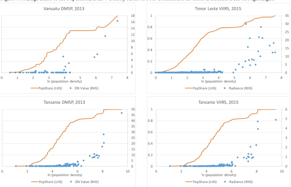
While VIIRS has finer spatial resolution and is more sensitive to dimmer lights, the VIIRS measurements occur around 1.30am, when most rural lights are likely to be turned off, given that few rural people are engaged in nocturnal activity needing light at these hours. The poor detection of lights for low-density (i.e., rural) areas is shown in Figure 7, for two small countries (Timor Leste and Vanuatu – both are in the lowest two data quality categories of Chen and Nordhaus (2011), so these are places where the lights data are potentially the most useful), and for Tanzania. In this figure, the population density (for either the second or third sub-national level) from the latest census is related to the cumulative population share and to the average DN value (from DMSP annual composites) or to the average radiance (from VIIRS) in the year closest to the census.
In Vanuatu, almost all areas register no light according to the satellites, despite being a country where rural households benefitted from a major development program over the last
21
decade. Specifically, seasonal migration to New Zealand lifted incomes 40%, with aggregate impacts equivalent to one-quarter of Vanuatu’s annual goods exports (Gibson and McKenzie, 2014). Income gains from seasonal work boosted the electrification rate; using census data for small areas, Gibson and Bailey (2020) find that a standard deviation (SD) higher seasonal work rate caused a 0.4 SD increase in the rate of having electric light (t=4.3). Yet despite this relationship in the micro data, neither VIIRS nor DMSP data show statistically significant correlations with these electrification rates nor with seasonal work rates.15 This example
shows that the sort of lights typically used in rural villages are not the type easily detectable from space, limiting the usefulness of satellite data on night lights for studying rural areas.
Figure 7 shows that little night light in Vanuatu and Timor Leste is found with either DMSP or VIIRS, for areas with population densities below 60 per km2. Such areas have over 60% of the population of Vanuatu and about 75% for Timor Leste. This is not from lack of electrification, as 55% of Timor Leste households in areas where the population density is below either 60, 50, 40 or even 30 persons per km2 use electricity as their main source of light according to the census. For Tanzania, areas with densities below 140 persons per km2 are generally not recorded as having night lights, for either VIIRS or DMSP (bottom panels of Table 7), yet such areas are home to about 70% of the population. The inability of DMSP and VIIRS to detect small, low density, settlements is also seen in Andersson et al (2019); out of 147 geo-referenced cities and towns in Burkina Faso, ranging in population from 1.6 million to 7000, 83 of these communities (the largest of which had a population of 32,000) went undetected over the entire 21 years of DMSP data. Indeed, only six of the ten largest towns and cities were detected in every year. Using VIIRS data (from two short periods in 2012) hardly raised detection rates (going from 40% to 45%).16
15 The participation rates in seasonal work are uncorrelated with population density (r=0.07) but there are high
correlations between population density and either the average DN value from DMSP for 2013 (r=0.83) or radiance data from VIIRS for 2016 (r=0.73).
16 Using the same VIIRS data for 2012, Chen and Nordhaus (2015) find a bigger improvement over DMSP
(using satellite F18 for 2010). For 600 cells (of 1×1) in Africa with population estimated to be below 10,000, all showed light using VIIRS but 72% of them showed no light with DMSP.
22
Figure 7: A Large Share of the Population, in Low Density Areas of Poor Countries, is Invisible in Satellite Data on Night Lights
0 5 10 15 20 25 30 35 0 0.2 0.4 0.6 0.8 1 0 1 2 3 4 5 6 7 8 ln (population density) Timor Leste VIIRS, 2015
PopShare (LHS) Radiance (RHS) 0 2 4 6 8 10 12 14 16 18 0 0.2 0.4 0.6 0.8 1 0 1 2 3 4 5 6 7 8 ln (population density) Vanuatu DMSP, 2013 PopShare (LHS) DN Value (RHS) 0 1 2 3 4 5 6 0 0.2 0.4 0.6 0.8 1 0 2 4 6 8 10 ln (population density) Tanzania VIIRS, 2015 PopShare (LHS) Radiance (RHS) 0 5 10 15 20 25 30 35 40 45 50 0 0.2 0.4 0.6 0.8 1 0 2 4 6 8 10 ln (population density) Tanzania DMSP, 2013 PopShare (LHS) DN Value (RHS)
23
Three more aggregate studies also find that night lights data better measure economic activity in the urban sector than in the rural sector. The first is of relationships between night light (annual averages of DMSP stable lights) and national GDP, for about 150 countries over 18 years (Keola et al, 2015). While the elasticity of light with respect to GDP is positive for countries where the agricultural share of GDP is less than 20% (with a weighted elasticity of 0.58), the elasticity becomes negative when the agricultural share of GDP is greater than 20% (with a weighted elasticity of -0.34). The authors note that it is possible for agriculture’s value-added to increase without an increase in the lights that are detectable by the DMSP sensors. Even with the more accurate VIIRS data, a similar effect is apparent. Chen and Nordhaus (2019) find that VIIRS lights have a closer relationship with GDP for metropolitan statistical areas (MSAs) in the United States than with state-level GDP and suggest that this is because the MSAs specialize in economic activity, like services and retail, that are more likely to be captured by night lights while in the non-MSA areas, activities like agriculture are less dependent on lighting at night. Relatedly, Gibson et al (2019) find that the elasticity of regional GDP with respect to night lights is almost 1.0 for urban areas of Indonesia, while the same elasticity for rural areas is negative when using the DMSP data.
In Table 2 we show further evidence that night lights relate more closely to economic activity in urban areas than rural areas. In this table we use the fact that prefectures in China are composed of two types of lower level units – districts (shiqu) that contain the urban core of the prefecture and have a mean resident population density of 1500 persons per km2 (from the 2010 census), and counties that are more rural with a mean population density of 300 per square km.17 The elasticity of lights with respect to GDP is over 0.3 for urban districts, but is less than three-fifths as large, with an elasticity of 0.19, for the counties (Table 2). This gap holds whether or not we control for population and area. The between-R2 values (which
usually exceed the within-R2, supporting the idea that lights are more accurate proxies for
economic activity in the cross-section than in the time-series) are also higher for the urban districts than for the counties. The difference in the lights-GDP relationship between districts and counties in Table 2 is likely to be smaller than the rural-urban gap in elasticities in many other settings, because China’s counties also include some urban areas (county-level cities), and some of the spatial units that are given an urban district designation have only recently
17 Results in this table exclude Leagues, Autonomous Prefectures, and Provincially Administered areas, which
are mainly found in western China and are distinguished by having no urban districts. These areas have much lower population densities than elsewhere in China and account for only about five percent of all residents. We also exclude 13 prefectures that are comprised solely of urban districts, to enable a balanced comparison of the relationship between lights and GDP for counties and districts within the same prefectures.
24
been upgraded from county status and still have quite low population densities.18
Table 2. DMSP Night Lights are More Closely Related to Urban GDP than to Rural GDP: China, 2000-2012
Dependent variable: ln(average DN value per km2)
it
Urban Districts Counties
(1) (2) (3) (4)
ln(GDP/km2)it 0.300 0.314 0.186 0.187
(0.046)*** (0.046)*** (0.033)*** (0.033)***
ln(population)it -0.230 -0.044
(0.067)*** (0.097)
Area fixed effects Yes Yes Yes Yes
Year fixed effects Yes Yes Yes Yes
Satellite fixed effects Yes Yes Yes Yes
Within R-squared 0.729 0.731 0.773 0.773
Between R-squared 0.756 0.908 0.684 0.792
Notes: Robust standard errors are in parentheses; * significant at 10%; ** at 5%; *** at 1%. N=5773. The contiguous districts within each prefecture are merged, to form the urban core used in columns (1) and (2), and the counties and county-level cities in the prefecture are merged to form the rural hinterland (n=273 for each type of spatial unit). Each spatial unit has 21 satellite-years of observations.
III.
Some Uses of Night Lights Data in Economics
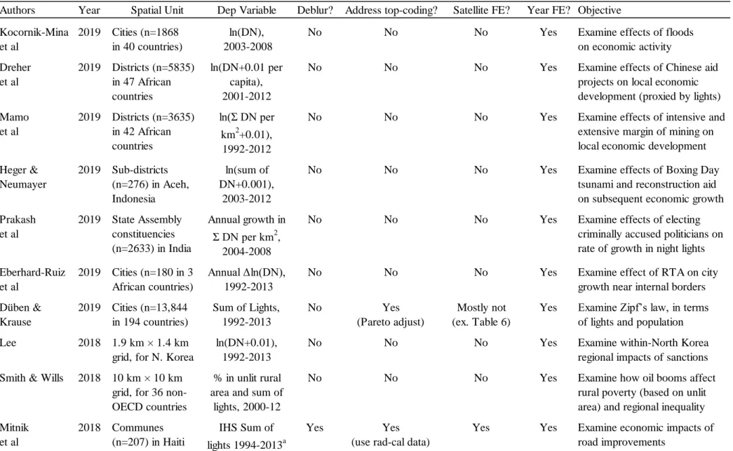
Our review of the sources of night lights data highlights several problems with DMSP data, so we now turn to a selective review of uses of these data in economics to see if, and how, these problems are dealt with. We review applied rather than methodological studies, so Abrahams et al (2018) and Bluhm and Krause (2018) are not further covered. We also restrict attention to studies that include observations from developing countries, either solely or in a database for many countries. While night lights are also used in applied economic studies that focus just on developed countries (e.g. Nguyen and Noy, 2018), developing countries often have fewer sources of evidence, and so flaws in the night lights data may do more harm to our economic understanding of developing countries because the research results that are based on night lights may have been more influential in these settings (given the paucity of other evidence).
We start by summarizing selected studies that have DMSP night lights data on the left hand side (LHS) of the relationships they estimate. We usually consider errors on the LHS to be less threat to the validity of an analysis, than is the case for errors in right hand side (RHS)
18 For example, the 90th percentile population density for the counties used in Table 2 exceeds the 35th percentile
density for the urban districts, showing an overlap between the two sectors that would be less apparent in many countries where metropolitan areas are functionally defined by density rather than by administrative boundary.
25
variables, for which random measurement errors cause attenuation bias in OLS regression coefficients. However, the measurement errors in DMSP data are almost certainly mean reverting – due to blurring that attributes light to places it is not emitted and top-coding that understates the differences in brightness between places – and mean-reverting errors in LHS variables cause coefficient bias (Abay et al, 2019, Gibson et al, 2015).19 Studies with DMSP
data on the LHS also more readily lend themselves to using satellite fixed effects, by choosing as the unit of observation (for panel analyses) the light recorded as coming from area i, in year t, by satellite s. This choice of the unit of observation saves one from either discarding data, noting that 12 of the 22 years in the DMSP time-series have records from two satellites, or from ad hoc averaging across satellites within a year.
Notwithstanding the potential to use satellite fixed effects, their statistical significance in the original Chen and Nordhaus (2011) study, and that they more precisely explain the time-series variation in national-level DMSP data than do year effects (see Section 2.2 above), most of the studies in Table 3 omit satellite effects. Some studies claim that year fixed effects will control for any unobserved satellite characteristics (e.g. Lee, 2018), but if this was true then satellite fixed effects would be statistically insignificant in the studies that have included them, yet they are not.20 In other cases (e.g. Eberhard-Ruiz et al, 2019) authors discard data from one satellite, in the years that have two satellites providing the data. It is unlikely to be optimal to throw away information when the annual changes in the data from one DMSP satellite can be quite different to the changes shown for the same place by the other satellite in orbit the same year (as Figure 6 exemplifies).
The same 12 studies in Table 3 that omit satellite effects, plus one cross-sectional study, appear to use no procedures for dealing with the top-coding of the DN values. This is despite several of the more recent studies having a focus only on cities, where the top-coding problems are most likely to matter. Amongst the studies that do deal with top-coding, two use the radiance-calibrated data, one relies on the Pareto-adjusted data, and one is based on a dummy variable for whether pixels are lit or not (and so it is censoring from the bottom rather than the top that may matter).
19 With a strong enough mean reversion, for mis-measured variables on the RHS, there can be exaggeration of
regression coefficients rather than the typical attenuation. The effects are even more complicated when errors are on both LHS and RHS (Abay et al, 2019).
20 For example, in the Table 2 results for China, which is a country where growth in DMSP-measured night
lights should have one of the highest signal-to-noise ratios of any country, because of the very rapid growth in urban lit area in the last two decades, the restrictions to omit the satellite fixed effects generate a chi-square statistic of over 3200 (p<0.0001). If satellite effects matter for China, they should matter even more so in less rapidly urbanizing settings, where the signal-to-noise ratio in the DMSP time series will be much lower.
26
Authors Year Spatial Unit Dep Variable Deblur? Address top-coding? Satellite FE? Year FE? Objective
Kocornik-Mina et al 2019 Cities (n=1868 in 40 countries) ln(DN), 2003-2008
No No No Yes Examine effects of floods
on economic activity Dreher et al 2019 Districts (n=5835) in 47 African countries ln(DN+0.01 per capita), 2001-2012
No No No Yes Examine effects of Chinese aid
projects on local economic development (proxied by lights) Mamo et al 2019 Districts (n=3635) in 42 African countries ln(Σ DN per km2+0.01), 1992-2012
No No No Yes Examine effects of intensive and
extensive margin of mining on local economic development Heger & Neumayer 2019 Sub-districts (n=276) in Aceh, Indonesia ln(sum of DN+0.001), 2003-2012
No No No Yes Examine effects of Boxing Day
tsunami and reconstruction aid on subsequent economic growth Prakash et al 2019 State Assembly constituencies (n=2633) in India Annual growth in Σ DN per km2 , 2004-2008
No No No Yes Examine effects of electing
criminally accused politicians on rate of growth in night lights Eberhard-Ruiz et al 2019 Cities (n=180 in 3 African countries) Annual Δln(DN), 1992-2013
No No No Yes Examine effect of RTA on city
growth near internal borders Düben & Krause 2019 Cities (n=13,844 in 194 countries) Sum of Lights, 1992-2013 No Yes (Pareto adjust) Mostly not (ex. Table 6)
Yes Examine Zipf’s law, in terms of lights and population
Lee 2018 1.9 km × 1.4 km
grid, for N. Korea
ln(DN+0.01), 1992-2013
No No No Yes Examine within-North Korea
regional impacts of sanctions Smith & Wills 2018 10 km × 10 km
grid, for 36 non-OECD countries
% in unlit rural area and sum of
lights, 2000-12
No No No Yes Examine how oil booms affect
rural poverty (based on unlit area) and regional inequality Mitnik et al 2018 Communes (n=207) in Haiti IHS Sum of lights 1994-2013a Yes Yes
(use rad-cal data)
Yes Yes Examine economic impacts of
road improvements Table 3: Selected Uses of DMSP Night Lights Data: Studies With Lights Variables on the Left Hand Side (most recent studies first)
27
Authors Year Spatial Unit Dep Variable Deblur? Address top-coding? Satellite FE? Year FE? Objective
Castelló‐ Climent et al 2017 Districts (n=500) in 20 Indian states ln(Σ DN per km2), in 2006 No Yes
(use rad-cal data)
No No Examine how higher education
affects economic development Corral & Schling 2017 Beachs (n=23) in Barbados ln(deblurred DN), 1992-2010 Yes No No Synth control
Examine local economic impact of shoreline stabilization
Villa 2016 Districts (n=732
in Colombia)
Annual Δ(ΣDN), 1998-2004
No No No Yes Examine how social transfers
affect local growth (in lights) Storeygard 2016 Cities (n=289 in 15 African countries) ln(Σ DN per city), 1992-2008 No Nob Partly (average within sat-year)
Yes Examine effects of transport costs on urban economic output Baskaran et al 2015 State Assembly constituencies (n=3800) in India ln(Σ DN+1 per capita),c 2001-2012
No No No Yes Examine political manipulation
of electricity supply during special elections
Gibson et al
2015 Cities (n=47) with pop>1m in India
ln(urban lit area), 1992-2012
No Yes
(min DN criteria)
Yes Yes Examine urban area growth and
change from prior land cover Hodler & Raschky 2014 Districts (n=38427) in 126 countries ln (DN+0.01), 1992-2009
No No No Yes Examine how the birth regions
of political leaders benefit (in terms of brighter lights) Michalopoulos & Papaioannou 2014 Cross-border ethnic homeland partitions (n=507) in Africad ln (mean DN+0.01), 2007-2008
No No No No Examine the effect of national
institutions on local economic development (lights), comparing across borders, within-ethnicity Table 3 continued : Selected Uses of DMSP Night Lights Data: Studies With Lights Variables on the Left Hand Side (most recent studies first)
Notes:
a
IHS is the inverse hyperbolic sine transformation
b
Uses a Tobit for bottom-coding
c
Also use annual growth rate of the sum of lights per capita, and share of villages with lights detected by DMSP
d
28
Several of the studies in Table 3 use observations for small spatial units, such as the grid over North Korea of 2.6 km2 used by Lee (2018) or the sub-district level in Aceh used by Heger and Neumayer (2019). Yet despite the code for the deblurring procedure of Abrahams et al (2018) being freely available since 2015, it is used by just one study in Table 3 that is based on very small spatial units – the beach-level study by Corral and Schling (2017). Whether the results for other studies based on small geographic units would change if researchers were using the deblurred data, or were using the even more spatially precise and accurate VIIRS data, remains an open question.
Another relevant feature of the spatial units in the Table 3 studies is whether the focus is on rural or urban areas. The discussion in Section 2.3 suggests that detecting night lights by satellites is more appropriate for cities than for rural areas, due to the type of lights that are needed (such as high pressure sodium lamps) in order to be detected from space and due to the underlying differences in population density that produce more concentrated sources of lights. A few of the studies in Table 3 focus only on cities, but many also cover rural areas, and some rely on rates of detecting lights for villages or rural areas as outcomes of interest (e.g. Baskaran et al, 2015; Smith and Wills, 2018). The national level findings from Keola et al (2015) and the regional level findings from Gibson et al (2019), that DMSP night lights are negatively correlated with GDP in times or places where agriculture is more important, raise some doubts about what effects are being identified when DMSP lights data are a proxy for village-level activity or for rural poverty.
Several of the studies in Table 3 rely on annual changes in, or growth rates of, DMSP night lights (e.g. Prakash et al, 2019; Villa, 2016; Baskaran et al, 2015). Yet prior validation studies find that changes in DMSP night lights data very poorly predict changes in economic variables (Addison and Stewart, 2015; Nordhaus and Chen, 2015). More recent validation studies collaborate this finding that changes in night lights are poor temporal predictors. For example, Goldblatt et al (2019) use commune-level data for Vietnam from 2004 to 2012, finding changes in DMSP night lights negatively correlate with annual changes in enterprises or employment, even as cross-sectional elasticities of these variables with respect to DMSP night lights were from 0.6 to 0.8. Relatedly, while DMSP data could explain one-third of the cross-sectional variation in enterprises and employment, they explained less than one percent of the variation in the temporal changes in these variables. Even when the more accurate (and temporally consistent) VIIRS night lights data are used, for metropolitan areas in the United States – so using the lights data for where they are best suited, in high density urban areas – Chen and Nordhaus (2019) find that the cross-sectional predictions for GDP based on the
29
VIIRS data have 88% predictive accuracy but there is just two percent predictive accuracy for annual rates of change in GDP. It is therefore unclear how much weight should be put on the various studies in Table 3, and other studies not summarized, that rely on annual changes in satellite-detected night lights data.21
A feature of the studies reviewed in Table 3, that is not apparent in the table, concerns citation patterns as an indicator of where researchers seek their guidance. First, twice as many of the studies cite Henderson et al (2012), compared to the citations to Chen and Nordhaus (2011), in line with what Figure 1 reveals more generally. A second pattern is that while the median number of studies referenced is 65, the median number of references to studies in the remote sensing literature is less than two. Indeed, more than one-quarter of the papers in Table 3 had no references to papers in the remote sensing literature. The insularity of
economics is well known (e.g. Fourcade et al, 2015) yet it is still surprising to find that when applied economists have ventured into using a data source that is fairly new to the discipline, and is based on data collection methods that are not covered in typical economics training (unlike, say, lectures on how National Accounts aggregates are constructed or on the design of sample surveys), they pay so little attention to findings from other disciplines that have long-standing and specialized knowledge about features of these data.
Most obviously, a greater reliance on the remote sensing literature might alert applied economists to the availability of potentially better VIIRS night lights data. Yet a text search of the seven papers from Table 3 that are dated 2019 – so allowing seven years from when VIIRS data were first available in 2012, and four years since the annual output of scientific papers that use data from the VIIRS Day-Night Band overtook the output of articles based on DMSP night lights data (Figure 2) – found not a single mention of VIIRS. Thus, the failure of applied economists to seek guidance from the remote sensing literature is potentially locking them into using a sub-optimal data source. Some defenders of the ongoing use of DMSP data may point out that it provides a longer time-series, and so persisting with this data source may be optimal, yet five of the studies in Table 3 are either cross-sectional or are based on a time-series of less than six years, which is shorter than the current time-series for VIIRS and so this defense does not really hold. Moreover, the DMSP time-series stopped in 2013 (and will not be continued), while the VIIRS time-series is getting longer every month (and lags
21 There is also a literature that relies on annual changes in DMSP night lights as RHS variables, for detecting
manipulation of reported GDP growth rates, which are the variables used on the left hand side (e.g. Chan et al, 2019; Martinez, 2018). This research design relies on the DMSP data being an accurate measure of the true change in economic activity and there is ample reason to question this, especially because of the lack of comparability of DN values over time discussed in Section 2.2.
30
real-time by only about three months) and so it seems that economists have invested in an increasingly outdated source of information while ignoring newer and better data from VIIRS (and from other remote sensing sources).
There are also more subtle ways that inattention to the remote sensing literature may be skewing economists’ understanding of satellite-detected night lights data. For example, a common misinterpretation in the Table 3 studies is that DMSP sensors can detect differences in light for areas of about one km2 size. For example, Baskaran et al (2015: 66) say “[t]hese
images record average light output at the 30 arcsecond level, equivalent to about 1 km2 at the
equator.” While the processed annual composites are allocated to grids of 30 arc seconds, the sensor resolution is much more coarse and so it is incorrect to say that light is recorded at a spatial resolution of 30 arc seconds. Absent geo-location errors, the smoothed pixels would cover about seven km2 at the nadir (2.7 km × 2.7 km) and over twice as much at the edge of the half-swath 750 km from the nadir; the boundary NOAA set for the usable images (as the FOV expands too much going further out). The geolocation errors, discussed in the remote sensing literature for almost a decade (Tuttle et al, 2013), further displace the signal by about three kilometres from where light is emitted. Thus, remote sensing experts like Elvidge et al (2013) describe DMSP as having a 25 km2 ground footprint at nadir, getting even coarser towards swath edges.22 If authors, editors, and referees in economics were more aware that the DMSP sensors record night lights at such a coarse spatial resolution, there might be somewhat greater skepticism about some findings that are, ostensibly, based on variation in data collected at the square kilometre level.23
Notwithstanding these data quality concerns, the range of topics studied with DMSP data highlight the potential value of accurate measures of luminosity. The studies in Table 3 include evaluations of local interventions, such as road improvements, shoreline stabilization and aid projects which are often difficult to study in the absence of ex ante data collection on baseline variables and so satellite-detected luminosity is useful because it potentially helps form a baseline for studies that are carried out ex post. Another useful aspect is for studies of sensitive things like political manipulation, regional favoritism, and the effects of other country actions on places – such as North Korea – where it would be difficult to trust the data provided by governments even if they had sufficient statistical capacity.
22 In contrast, the VIIRS ground footprint is 45 times smaller at nadir and even smaller towards the swath edge. 23 The beach-level study of Corral and Schling (2017) that has the smallest spatial units in Table 3 uses the
31
In addition to studies with variables derived from DMSP lights data on the left hand side, several studies have lights variables on the right hand side. We do not table a summary of these studies, because in some cases (a subset of, or a variant of) the data used as the LHS variables in the studies in Table 3 are used as RHS variables in other studies by the same authors (e.g. Hodler and Raschky, 2014a; Dreher et al, 2019a). Thus there may be similar issues with respect to blurring, top-coding, and the other sources of measurement error. One standalone study with lights variables on the RHS that shows the threat posed by flaws in the DMSP data is Gibson et al (2017), who examine effects of urban growth on rural poverty in India; big city lights are contrasted with lights from towns, and for both the extensive margin (lit area) is contrasted with the intensive margin (brightness of the lit area). It seems that only growth on the extensive margin, and especially in towns rather than big cities, reduces rural poverty. While there are good reasons for such patterns, top-coding of the DMSP data also could cause this pattern if the extensive margin of lit area is measured more reliably than the intensive margin of brightness, especially noting that the earlier remote sensing literature settled for simpler extensive margin measures, such as whether pixels are lit brightly enough or not to be counted as part of the urban area (Henderson et al, 2003).24
IV.
Conclusions
Applied economists have been busy in the last few years using satellite-detected night lights to examine important research questions, especially in developing countries where it is likely that conventional economic statistics, such as national or regional GDP, are unavailable or inaccurate. Further growth in use of night lights is likely, as lights data have been included in the AidData geo-query tool for providing sub-national data, and in the geographic data that the Demographic and Health Survey links to anonymised survey enumeration areas. Yet it is arguable that applied economists have been insufficiently critical in their use of night lights data, especially because of their reliance on the DMSP data that come from sensors that were not designed to provide long-term, temporally consistent, and spatially precise, measures of lights on earth. The unsuitability of DMSP data for many research purposes has seen a rapid switch in other disciplines towards using the newer and better VIIRS night lights data. In particular, DMSP data are unsuitable for studying small areas, or border effects, because of
24 Gibson et al (2019) show that in another big city (Jakarta in 2012), 82% of pixels have the top-coded DMSP
value (DN=63) and 17% get DN=62. By treating all areas of a big city as roughly equally bright (while VIIRS shows much more intra-city variation in brightness) the DN value from the DMSP data is almost like a dummy variable for whether the pixel is part of the big city or not, raising the question of whether the intensive margin can be measured reliably by DMSP data.