Design and control of a semi-passive, heavy-duty paired mobile robot system with application to aircraft wing assembly

Design and Control of a Semi-Passive, Heavy-Duty Paired Mobile Robot

System with Application to Aircraft Wing Assembly

by

Manas Chandran Menon

B.S. Bio-engineering, The University of California, Berkeley (2003)

S.M. Mechanical Engineering, Massachusetts Institute of Technology (2008)

S.M Electrical Engineering and Computer Science, Massachusetts Institute of Technology (2008)

Submitted to the Department of Mechanical Engineering in partial fulfillment of the requirements for the degree of

Doctor of Philosophy at the

MASSACHUSETTS INSTITUTE OF TECHNOLOGY

September 2010 MASCUSNTT1S INSTITUTE OF TECHNOLO('Y

NOV 0

2010

LIBRARIES

ARCHNES

Author... A u t h o r ..... ... ... ....... ......... ... ... .... ..... ... ... ... .... .. .. . ... .. ... .... D.. .. ... ... f... .. ... .. . I... .... .i.. .. n.. .... ..n... JDepartment of Mechanical Engineering June 25, 2010 - / ,/ C, Certified by ... Accepted by ... . . . Graduate Of H. Harry Asada Ford Professor of Mechanical Engineering Thesis Supervisor

David Hardt ficer, Professor of Mechanical Engineering

Design and control of a heavy duty paired mobile robot system with

application to aircraft wing assembly

By

Manas Menon

Submitted to the Department of Mechanical Engineering on June 25, 2010, in partial fulfillment of the

requirements for the degree of Doctor of Philosophy

Abstract

We describe the development of a robotic system capable of performing a class of

manufacturing operations. An example of such an operation is commonly found in aircraft assembly -this demonstrates the immediate applicability of -this research.

The system utilizes a unique concept - a pair of mobile robots acting on opposite sides of a thin wall. The robots interact with one another through the use of magnetic fields that penetrate this wall. The 'inner' robot is untethered and is controlled by the 'outer' robot. Despite the significant mass of the

outer robot, it operates without the aid of physical external supports.

Full modeling of the system is presented. We include calculations for forces and torques produced by sets of permanent magnets for any system state. Simplified, tractable versions of this model for the purpose of control are also described.

The system is designed to execute closed loop fine position control and large scale locomotion. Experimental results from a functional prototype verify the effectiveness of the design as well as the robustness of a position controller. Numerical optimal control results have been developed for high speed point to point trajectory motion.

This 'pair of robots' paradigm could be applicable to a variety of tasks. This work outlines analysis techniques that are useful for such a system at most scales.

Thesis Supervisor: H. Harry Asada

Ford Professor in Mechanical Engineering Thesis Committee

Steven Leeb

Professor, Department of Electrical Engineering and Computer Science Maria Yang

Acknowledgement

I'd like to extend my thanks to the Boeing Company for sponsoring my research. It is because of

their financial support and flexibility that I have been able to work on such an interesting and stimulating project, and I greatly appreciate it.

I would never have come to MIT, and certainly would not have been able to survive here, were it

not for all of the educators and experiences leading up through my undergraduate education. Though they are too many to name here, I must thank the teachers that inspired me through grade school and UMTYMP and my time at UC Berkeley. I would like to acknowledge especially Professor Ron Fearing and his lab in the EECS department at Berkeley for a great undergraduate research experience.

My advisor, Professor Harry Asada, has been an incredible instructor and mentor to me. His

creativity is invaluable when I get stuck and inspirational when I'm discouraged. His practicality, doled in measured doses, brings me back to earth when I need it most. He never allows me to settle for

mediocrity and has helped me to become a better engineer and researcher, and more importantly, a much more careful and critical thinker. The other members of my thesis committee, Professors Steve Leeb and Maria Yang have provided excellent advice in their areas of expertise, helping to round out my work in a way that would have been impossible on my own. Professor Marcus Zahn has also set aside time to meet with me and contributed significantly to my understanding of magnetic fields and forces.

My fellow lab members are a constant source of wisdom and insight as well as an often needed

comic relief. I have never had the opportunity to work with so many selfless, creative, motivated and intelligent people as I have these past few years and I'm honored to be considered their peer. In particular I would like to recognize Geoffrey Karasic, Anirban Mazumdar and Binayak Roy, who were my colleagues on the Boeing project for several years, as well as the undergraduate researchers I

supervised: Albert Wang, Matt Robertson and Todd Zusman.

Last, but certainly not least, I'd like to thank my family, especially my parents. It is difficult to put into words the gratitude I have for the way they have raised me. They are constant role models and teachers. They have given me an appreciation for math and science, food and art. They have taught me the importance of compassion and work ethic. They have given me the opportunity to live a full, happy

Table of Contents

.

...

1.1. M otivation ... 17

1.1.1. Futu re factory ... 17

1.1.2. Fastener installation ... 17

1.2. Previ ous work ... 18

. Design ). ... 20

11.1. Functional requirem ents ... 20

11.2. Previous designs ... 21

11.2.1. Spider robots ... 22

11.2.2. Piezo crawler ... 23

11.2.3. Inchworm walker... 24

11.2.4. M ultifunctional foot and resulting designs ... 27

11.2.5. Single degree of freedom system ... 30

11.2.6. Unsupported system - asym m etric oscillation ... 33

11.3. Design of choic e ... 34 11.3.1. General description ... 34 11.3.2. Architecture .. ... 35 11.3.3. M agnet selection... 36 11.3.4. Coil selection ... 37 11.4. Prototype ... 40 1ll. M odeling... 44

111.1. Full system model ... 44

111.1.1. Assum ptions ... 44

.1.2. M agnetic forces ... 47

111.1.3. Eddy dam ping ... 54

111.1.4. Reaction forces ... 59

111.2. Sum m ary ... 72

IV. Control

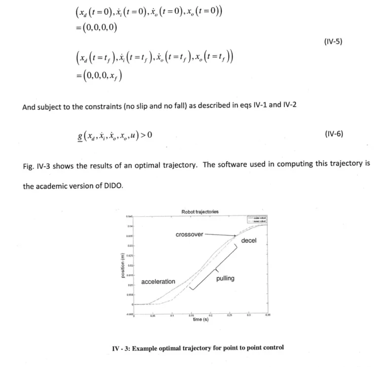
IV.1. Point to point optim al control ... 74

IV.1.1. Control strategy ... 74

IV.1.2. Key issues ... 74

IV.1.3. Simplified modeling and control for point to point optimal control ... 75

IV.1.4. Further discussion ... 78

IV.2. Fine positioning ... 83

IV.2.1. Contro strategy ... 83

IV.2.2. Key issues ... 85

IV.2.3. Sim plified m odeling and control for fine positioning ... 85

V.2.4. Further discussion ... 89

V. Conclusion ... 91

V.1. Sum m ary of contributions ... 91

V.1.1. Applicability ... 91 V.1.2. Novel design ... 91 V.1.3. Prototype ... 92 V.1.4. General m odel ... 92 V.1.5. Fine positioning ... 92 V.1.6. Gross positioning ... 92 V.2. Future w ork ... 93

V.2.1. Hall effect safety sensors ... 93 5

V.2.2. Obstacle avoidance ... 93

A. M ATLAB m odeling...94

B. M ATLAB initialization ... 108

List of Figures

I

automation of fastener installation

II - 1: Sketch showing the flange location on a wingbox. Two sets of tooling, one on the outside of the wingbox and one on the inside are required for this task.

II - 2: Concept sketch of pair of spider robots. These robots attach themselves to the skin utilizing magnetic attraction through the skin to one another.

11 - 3: Sketch of piezo activated positioning stage. The stage should be able to control angle to align the

tooling normal to the skin surface. It may also be required to do fine positioning.

11- 4: Sketch and photograph of piezo crawler prototype.

11 - 5: Explanation of locomotion for piezo crawler. Phase shifted sinusoidal trajectories at the 'knee'

and 'hip' cause rotational movement at the foot, which in turn cause net motion.

I - 6: Inchworm walker prototype. Pneumatic actuators were used to raise and lower feet and a lead

screw actuator was used to translate the feet relative to one another. II - 7: Inchworm walker outer foot, disassembled from the complete robot.

11- 8: Inchworm walker inner foot, disassembled from the complete robot.

11 - 9: Multifunctional foot demonstrating clamping and rolling. By changing the normal force only

slightly, the frictional properties of this foot would change dramatically. This allowed for a system to be held strongly in place (against gravity) yet translated (perpendicular to gravity).

I - 10: CAD model and photograph of multifunctional foot. This foot successfully demonstrated the

functionality desired.

II - 11: Two degree of freedom linear motion pair of robots. This model was realized in CAD only. II - 12: Single degree of freedom pivoting foot system. This system has two 'feet' and is able to actuate through the use of a motor at the 'ankle' joint. A passive version of this system was built.

I - 13: Multi-foot swinging robot utilizing compliance. This system was never fully realized. Ideally,

resonances in the system due to mass / springs would have been exploited. Unfortunately, eddy current damping would likely have made such a plan infeasible.

II - 14: Architecture of single degree of freedom system. This figure shows the location of the magnetic fields from the permanent magnet mounted on the inner robot.

ll - 16: This figure shows the location of the electromagnet and steel plate used to demonstrate the

clamping functionality of the system.

II - 17: CAD drawing of the single degree of freedom prototype showing the location of all components in the prototype

il - 18: Single degree of freedom prototype with labeled parts. The electromagnet and wire coils are hidden behind a mask.

II - 19: Plot showing the fine positioning ability of the single degree of freedom system. This demonstrated the effectiveness of using a Lorentz force for fine positioning.

II - 20: Diagram showing the forces on the unsupported system

II - 21: Forces on the moving unsupported system - this shows the nonlinear forces that result from a non-zero velocity

11 - 22: Side view of the chosen design. The inner and outer robot are separated by a thin aluminum skin. From this view it is possible to see the alignment of permanent magnets between the inner and outer robots as well as the alignment between the magnets on the inner robot and the wire coil on the outer robot

11 - 23: Top view of the chosen design. This view shows the layout of the permanent magnets and coils

relative to one another.

11 - 24: Effect of number of magnets on holding stability. This figure shows the difference in safety

between having three magnet banks (minimum number necessary) and four magnet banks (allows for more safety). We chose to have four magnet banks on the prototype for this additional safety

II - 25: Halbach array. This figure shows the location of flux concentration as well as the location of reduced flux concentration for a Halbach array

II - 26: CAD model of 'magnet bank.' This is the basic magnetic building block used in this system. Aluminum housings were used for strength and rapid prototyped plastics were used for alignment. Assembly of these magnet banks was relatively straightforward.

11 - 27: Lorentz force direction given a direction of current and a direction of flux.

11 - 28: Lorentz force proof of concept demo. This simple setup was built to test that the Lorentz force

we would be able to generate would be of appropriate order of magnitude for the application. The left side of the picture shows a fixed coil of wire. The right side shows a magnet mounted on a vertical linear rail. By driving the coil with an oscillating current we were able to observe oscillations in the magnet on the right side of the photo.

11 - 29: Image taken from an FEA to find the flux in the coil. This was used only as a rough order of

magnitude estimate to chose coil and core size.

11 - 30: Use of laser to align robotic system. This figure shows how a robot mounted position sensitive

device (PSD) can be used to locate a laser (the laser in this case would be mounted on a fastener, or fastener location).

11 - 31: Beam splitter and mirror setup used to create a low form factor bi directional laser. This device

was very useful for testing with our prototype.

11 - 32: CAD model of functional prototype. Components are marked.

11 - 33: Outer robot prototype suspended upside down. It is held in place through the skin due to

magnets on the inner robot. II - 34: Inner robot prototype.

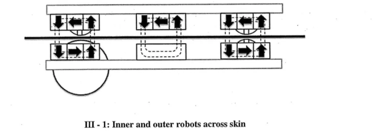
II - 1: Inner and outer robots across the skin

11 - 2: Inner and outer robot represented as rigid bodies. Note that the outer robot rear wheel contact

is not marked - this is instead considered constrained to a plane. Inertia of the wheel on the outer robot is ignored.

III - 3: Definition of several components of the state

III - 4: Magnetic charge model description. Magnetic north and south pole faces are represented by

areas with some 'magnetic charge.'

11 - 5: Left image shows the fields due to single magnet. The top and bottom (north and south) poles of

the magnet are shown as squares. Right image shows the fields due to a Halbach array. Again, north and south poles of the three magnets in the array are shown as squares. In both cases, to help visualization, the fields are only shown on a plane just above and below the magnet.

III - 6: For Maxwell's stress tensor, we must create a surface around one Halbach array and evaluate the

magnetic fields at all locations at this surface. This figure shows the surface automatically chosen by the code and the fields at that surface.

IlIl - 7: CAD showing setup in the Admet machine to find normal forces between a pair of Halbach arrays.

III - 8: Normal force measurements as a function of displacement for two different magnet grades.

IlIl - 9: Comparison of simulated forces for a pair of Halbach arrays to the experimental data. Note that

the simulation data was scaled to fit the experimental data at the minimum distance location (this corresponded to around 3 mm). After this scaling, however, the two curves matched well. This suggests that a reasonable design method is to measure the forces between a pair of magnets, use this

information to set the 'assumed magnet grade' (basically use this as a scaling factor) and then run analyses with this assumed magnet grade.

Ill - 10: Lateral restoring force versus robot misalignment, found in simulation.

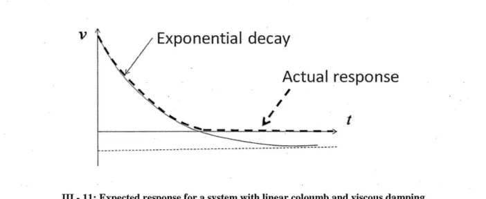
Ill - 11: Expected response for a system with linear viscous and nonlinear coulomb damping

11 - 12: Experimental results in the two cases (1) with eddy current (2) without eddy current

11 - 13: Experimental data compared to an exponential curve fit (which would be expected in the case of

linear viscous damping). The curve fits very well.

Ill - 14: Drawing showing the possible effect of eddy currents caused by motion of the inner robot

affecting the force on the outer robot.

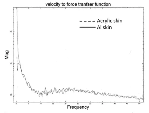
II1 - 15: Transfer function between velocity of inner magnet to force on outer magnet (forces due to

trans-skin eddy effects) showing little difference between acrylic skin and aluminum skin. This suggests we can safely ignore these trans-skin effects.

Ill - 16: Diagram labeling dimensions on the outer robot.

Ill - 17: Diagram labeling dimensions on the outer robot.

IlIl - 18: Components of forces on magnet banks.

111- 19: Components of torques on magnet banks.

11 - 20: Reaction forces on outer robot. Note that reaction forces occurring at the rear axles signify that

we ignore inertia of the wheels.

Ill - 21: Free body diagram showing the effect of ignoring inertia on the rear wheels of the outer robot.

Il - 22: Outer robot chassis tilt found using assumed compliance in wheel elements. This is applied in

the method of deformations.

III - 23: Total deflection of compliant elements, outer robot. This is applied in the method of

deformations.

III - 24: instantaneous center of rotation of the outer robot is along the axels of the rear wheels. This is

due to the applied no slip condition at these wheels. Ill - 25: Diagram labeling dimensions on the inner robot.

Ill - 26: Diagram labeling dimensions on the inner robot.

III - 28: Reaction forces inner robot.

Ill - 29: Inner robot chassis tilt found using assumed compliance in wheel elements. This is applied in the method of deformations.

Il1 - 30: Total deflection of compliant elements, outer robot. This is applied in the method of

deformations.

IV - 1: Strategy for point to point control of outer robot. First the pair of robots turns to align with the desired endpoint. Next, the pair of robots drives towards this endpoint in a straight line.

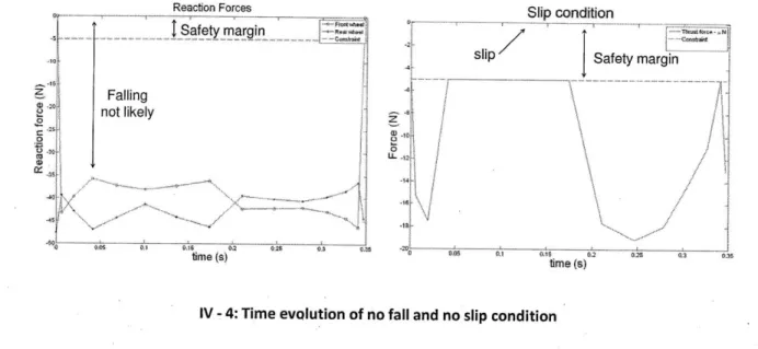
IV - 2: Reaction forces and their relationship to no slip and no fall conditions, outer robot.

IV - 3: Example optimal trajectory for point to point optimal control. Note that the outer robot initially leads the inner robot, until, near the end of the trajectory, it slows to let the inner robot pass. This allows both robots to quickly reach the desired endpoint with zero velocity.

IV - 4: No fall and no-slip conditions during execution of this optimal trajectory (in simulation). Note the safety factory added to each condition. Also note that the no-slip condition is far more strict.

IV - 5: Maximum torque the outer robot can apply before slippage or falling. The white region is the region in which, even at zero torque, the robot will fall. At (a) and (b), the robot falls due to reduce magnet holding forces because of gross misalignment between the inner and outer robots. At (c) and

(d), the velocity is large enough to cause significant eddy current forces on the outer robot, applying a

torque that peels it off the surface.

IV - 6: This figure describes in more detail how high velocities can cause eddy forces causing a torque that helps peel the outer robot from the surface.

IV - 7: Allowable motor torques before slippage or falling for different coefficients of eddy current damping.

IV - 8: Allowable motor torques before slippage or falling for normalized position and velocity. This is independent of eddy current.

IV - 9: Region in which not only torque can be applied, but direction of acceleration can be influenced, for two different values of eddy current damping.

IV - 10: Description of inverse kinematics that must be solved for to get some desired velocity direction. IV - 11: Lumped parameter modeling for fine positioning.

IV - 12: Root locus for fine positioning of inner robot.

IV - 14: Inner robot following a ladder - type reference trajectory.

IV - 15: Coupling between axes. Top plot shows x direction motion while bottom plot shows y direction motion. Note that a step in one axis causes a disturbance in the other.

List of tables

List of Abbreviations and Symbols

Gross motion analysis

x0, y0, 0 : x position, y position, orientation of outer robot in outer robot frame

Xd, YdOd : relative x, y positions and orientation of inner robot in outer robot frame

a1,a2, a3: coordinate frame fixed to outer robot

6 _,,#2,A8

3: coordinate frame fixed to inner robot

vowlvow2,vow3,vow~v,,w, viw2,viw3,viw4: velocities of outer, inner wheels in outer robot frame

X

jdd,

Xd : a _{vector containing xd, yd, Od}

m, m2,

, m

,

m

, n7,m

,

m

:

outer robot dimensions

ni,n 2,n3,n4,n.,n8 outer robot dimensions

m,,m : mass inner, outer robot

Ic: 2 moment around center of mass

g : gravity

R1X, R0 4x, Ro0y, R.2,, R y,, , R,4 R , Ro 2 , R03z , R04z: reaction forces outer robot

&i, 02

,

,

:

reaction force vectors outer robot

ReX, Ri2x,

:

R, Ri2

,

reaction force vectors inner robot

Moz I Mo2zI Mo3z, Mo4 , MoIxMo2xMo3xMo 4x, Mo1 ,, M o2y M 3 ,, Mo4,: outer magnet forces

M

,

MA, Mi2,A'MMi3, 4: inner robot magnet vector forces

Tolz ' To2z 1o3z I "o4z' o1x2,1 o,1 o4x,1 ol y' I02y , T03y' I04y :

outer

magnet

, 1L2, o3' o : outer magnet torque vectors

r"motor2 Imotor3: motor torques

ilz ITi2z ,i3z ,i4z'

TilTi2x'TxTi4x

Ti2y' Ii3y

:

inner magnet

torques

1, -2,43,44: inner magnet torque vectors

Note: all magnet torques forces w.r.t. coordinate frame located at outer robot

rEm1,

r

rw1 ,w2 Iw3' Irw4 : vector from outer robot COM to outer robot wheel contact points

r , rv2,!4w3,!-w4: vector from inner robot COM to inner robot wheel contact points

rmi,5m2,4m3,5m4,5-1,5-2,5.3,5-4:

B A : vectors from outer robot wheels to tool location

Note: wheel, magnet location vectors in coordinate frame attached to corresponding robot

c: rolling resistance coefficient

Cr: coefficient of friction for rubber wheels

AO1, A0o2, os Ao4: small deflection of the outer robot wheels in the upward (+z) direction Aj1, i2, Ai3, Ai4 : small deflection of inner robot wheels in the downward (-z) direction

A0C, ACe: offset deflection for the entire chassis (see figure)

ao,bo,

a,,b,

ko,ko

, ko

, ko

:

stiffness's of outer robot wheels

k

,kj

,k

,

,

,k,4:

C,, (Xdx), CO, (X, Co9 (Xd ,,1k): coulomb friction in x, y, theta directions, outer robot

C,

(X~,,),

(Xd,),

(Xak):

D,,

(x),D, (k),D

(X):

D,

(x),

(x),D,

(X):

VRx (Xd),VR, (Xd),VROO (Xd): variable reluctance force in x, y, theta directions, outer robot

VRx

),VR,,

),

IF,,, F, i-: sum of forces in x, and y, sum of moments in theta, outer robot 1F~, ,IF,: sum of forces in x, and y, sum of moments in theta, inner robot

Fine positioning analysis

(xI, y

)

(x

k

,

b1,b2: viscous damping on outer, inner robot

kP,kd,k, : proportional, derivative, and integral control gains for PID controller F,, F : force in x, y direction from Lorentz force

I. Introduction

1.1. Motivation

1.1.1. Future factory

Dealing with volatility is one of the greatest challenges in the aircraft manufacturing industry [21,241. Tremendous resources are expended maintaining empty facilities during recessions and building temporary assembly stations in regions experiencing transient economic growth. This problem demonstrates a clear need for factories that can quickly and cheaply be constructed and taken down, or transported. Such a task is difficult because current facilities use large, heavy fixtures such as scaffolding

as an integral part of the manufacturing process.

A future factory concept devised in collaboration with our research sponsor is that of a manufacturing

facility devoid of such bulky components. Such a factory would start as a large empty hangar outfitted with a sensor array. Raw materials and partially assembled components would be brought in and assembled into more finished parts such as complete wings. This assembly would be carried out by self-supported, mobile robotic systems that could be easily transported to any such facility on the globe. Our aim is the development of a type of robotic system that enables such a paradigm shift in aircraft manufacturing.

1.1.2. Fastener installation

Fastener installation is an assembly operation that could benefit greatly from automation, and is therefore an excellent starting point for our efforts towards this future factory. Fasteners are pieces of hardware used to join two or more components such as sheet metal or flanges. There are on the order of several hundred thousand fasteners on common aircraft wings. Proper installation of these fasteners

is a two sided operation - on one side a hole is drilled, deburred, and the fastener inserted, while on the opposite side the hardware is braced against the drill and a nut or sleeve is attached to the inserted fastener.

The nature of this operation requires a thin skin of material separating the tooling on either side of the operation (in our case, the aluminum skin of the airplane wing). In order to maintain structural integrity of the wing, the fasteners must be precisely located. The tooling that performs this operation must be capable of undergoing a long stroke - on the order of the size of an airplane wing. Part of the fastener installation procedure requires a clamping force across the skin. In addition, some of the existing tooling for this operation is heavy, and must be supported.

As there is a great deal of existing tooling for the tasks in fastener installation (drilling, deburring, etc), we are interested in providing a robotic platform that enables these tools to perform their tasks in an autonomous manner. We are interested in positioning, locomotion and load bearing. Our overarching goal is to design a system that can enable fastener installation within the non-supported, mobile robotic framework necessitated by the 'mobile factory' paradigm.

1.2. Previous work

Fastener installation is currently performed by hand. A worker crawls inside the wingbox and uses a tool to slip nuts or sleeves over fasteners, mating with a tool on the outside of the wing. This operation is uncomfortable and dangerous for the worker. Previous attempts at automation have consisted mainly of variations on an articulating snake-like robot arm that could enter the wingbox through an access hole [9,34,35].

Inside

wingbox

skin

Outside

wingbox

II. Design

11.1. Functional Requirements

This robotic system is motivated by a real need in the aircraft industry. While we are interested in developing a system with general applicability, it is important to first address the specific needs of the motivating application.

As previously mentioned, fastener installation is a two sided process. The steps involved in the process are:

- Position tooling

- Clamp skin to flange

- Drill and countersink hole while removing chips

- Visually inspect the hole

- Insert fastener

- Seat fastener

- Add nut or sleeve to fastener (this depends on which type of fastener is being used)

- Release clamping

Outer tooling operations

U - 1: Flange location

This pair of tools requires some clamping functionality across the skin. For fastener installation, accuracy on the order of 100 um is needed. Additionally, the tooling should be able to move from hole to hole, potentially traversing large distances. The holes are located at distances on the order of several cm. The tooling may be called upon to travel the length of a wing, on the order of up to 30 m. The

system needs to be able to deal with heavy tooling - current systems on the outside of the plane weigh on the order of 100 kg; 1000 N holding force is required. Whatever positioning system we use must be capable of overcoming static friction effects caused by 1000 N of magnetic clamping force. Later, we show that a force of approximately 50 N is required for fine positioning. Finally, the robotic system on the inside of the wing should be able to operate within a cluttered environment.

It is worth noting that the tooling to perform the fastener installation operation already exists. It only remains that we develop a system capable of delivering the tooling precisely to some location and supporting it while it works. This robotic system is in a sense a generic tool delivery system for operations of this kind. It is also easily able to perform auxiliary tasks, such as clamping.

As previously mentioned, there are several groups attempting to automate this process by developing articulated snake-like robot arms. Our approach differs in that we intend to use a pair of robots that work together across the skin. These robots would stick to each other through the skin using magnets. Furthermore, we would like one robot (the master) to manipulate the other (slave). Non contact power transmission has been shown effective in several other applications [8,10,12,18,38]. This section describes some of the alternative designs considered within this framework of a pair of mobile robots utilizing magnets.

11.2.1. Spider robots

Our initial approach was the development of a pair of fully articulated robots acting across the skin as shown in Fig. 11-2. Each leg would have an electromagnet in order to be able to clamp

/

II -2: Pair of spider robot

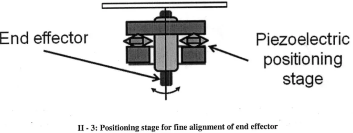
Gross position could be achieved by articulation of the legs, but fine positioning with such a system would likely be difficult. Several schemes for fine positioning were considered, including the addition of

a fine positioning stage to the end effector of the robot. High stiffness, short stroke piezoelectric actuators could be used to precisely position the tooling as desired.

End effector

Piezoelectric

positioning

stage

II - 3: Positioning stage for fine alignment of end effector

Unfortunately, it became quickly apparent that such a system was needlessly complex and would likely be too heavy to support itself against gravity.

11.2.2. Piezo crawler

Some development was made in the direction of a mobile robot powered by piezo electric actuators. Fig. 11-4 shows a CAD model and photograph of the finished prototype.

This three legged robot had two actuators per leg. By running these actuators out of phase or asymmetrically, net work could be created at the output of each leg, as shown in Fig. 11-5.

HiP

Knee

t

II - 5: Two degree of freedom foot

We were successful in achieving precise positioning control with this prototype. Unfortunately it would be unable to handle heavy tooling, and the functionality of the piezoelectric actuators do not scale up well to deal with forces present in the real system.

11.2.3. Inchworm walker

The next iteration prototype was built to prove that off the shelf permanent magnetic forces would be sufficient to hold up a heavy duty tool (which in the case of fastener installation can weigh on the order of 100 kgs). Fig. 11-6 shows the robot.

H - 6: Inchworm walker prototype

The robot was composed of two main sections. Each section had a 'foot' with a series of permanent magnets on its underside (see figures below). The robot hung upside down, supporting its own weight due to an attraction force between its magnets and blocks of steel placed inside the wingbox mock-up. This holding force was induced over an aluminum skin thickness of 1/8" - a common value in airplane wings.

A lead screw was used to actuate the relative displacement of these feet. By lifting the 'outer' foot,

displacing it forward, and then lowering the foot, the robot effectively took a step forward. This inchworm locomotion demonstrated a safe, albeit slow, method of locomotion for such a system.

Linear guides

Permanent

magnets

1 - 7: Inchworm walker outer foot

The inner foot is nested within the outer foot -this allows for the robot to remain stably attached when either foot is in contact.

-- guides

Magnet

locations

II -8: Inchworm walker inner foot

Having demonstrated the effectiveness of magnets to hold such a system against gravity, we were interested in making the mobile robots more nimble.

11.2.4. Multifunctional foot and resulting designs

A multifunctional foot was developed. It has the ability to clamp strongly to a surface or release and roll

with very little friction [27]. Fig. 11-9 shows the concept. A spring loaded magnet has the ability to engage or release a set of wheels. The position of the magnet is dependent on the pulling force on it (through the skin) as well as the force the spring exerts. This means that by modulating the attractive force with an electromagnet only slightly, we can change the state of the foot while still maintaining substantial normal forces. This allows us greatly modulate frictional properties of the foot (rolling coefficients of friction are often two orders of magnitude higher than sliding friction coefficients) while

maintaining a relatively constant attractive normal force.

Rolling mode

Fixed mode

clearance

Caster wheel

High friction

H - 9: Multifunctional foot demonstrating clamping and release

Spring in

housing

Pivot

Magnet

+

-- -

_-Wheel

_---..

_--

₊

II - 10: CAD model and iuinctioial prototype of multifunctional foot

This attaching / _{detaching foot concept allowed spurned the development of several new designs. We} imagined a pair of robots in which two linear motors could control the X Y position of the tooling, while the feet clamped or unclamped as desired for locomotion.

II -11: Two DOF linear motor pair of robots

A similar concept was a single pair of feet with rotary motors as the joints. Positioning would be more

II - 12: Single DOF pivoting foot system

A more complex design utilizing these multifunctional feet involved a series of legs, potentially with

linear springs, allowing us to exploit the dynamics of the system. These dynamics would change depending on which feet were attached, potentially leading to interesting behavior.

11.2.5. Single degree of freedom system

We settled on a relatively simple, yet robust and easy to control concept, shown in Fig. 11-14, as a precursor for the final design. In this system, the outer robot is supported by a gantry and has an electromagnet as well as a series of wire coils. The inner robot has steel plates mating with the outer electromagnet, as well as permanent magnets that mate with the wire coils.

Magnet banks Steel plate Inside wingbox Flux lines skin Outside wingbox Wire coils

II -14: Architecture of single DOF system

By running a current through the coils, equal and opposite Lorentz forces are induced on the pair of

robots. This allows us to perform fine positioning.

Current through

coils-.induces force on inner robot

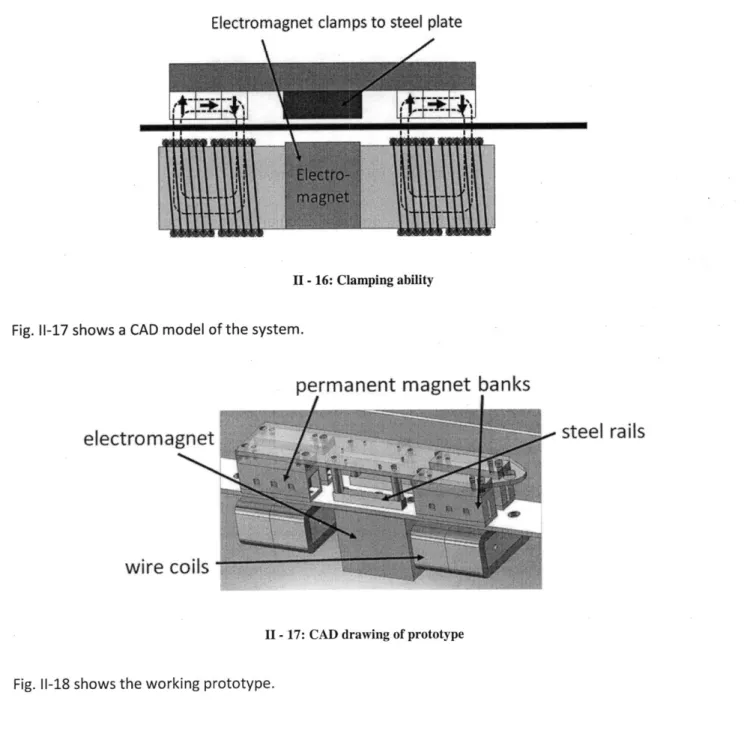
This system also demonstrated clamping functionality, as the steel plates were able to clamp to the electromagnet through the skin.

Electromagnet clamps to steel plate

II -16: Clamping ability

Fig. 11-17 shows a CAD model of the system.

permanent magnet banks

I I

,--

steel rails

electromagnet

wire coils

II -17: CAD drawing of prototype

Fig. 11-18 shows the working prototype.

permanent magnet banks

electrornagnet

steel

rails

wire coils

II - 18: Single DOF functional prototype

This system showed excellent ability to precisely position the inner robot. The outer robot is affixed to a gantry to support its weight and controlled by a leadscrew. At this point, we were not interested in servoing the outer robot, as control of the inner robot using the Lorentz force coil from across the skin is a much more interesting and challenging problem.

Servoing ability p aifr o robots

Reference Outer robot Inner robot

tme (s)

II.2.6. Unsupported system

-

asymmetric oscillation

Removing the support gantry used in the previous prototype is extremely advantageous in terms of flexibility and cost in manufacturing. In order to remove this support, it is important to apply a high magnetic holding force (normal to the skin) to support the outer robot against gravity. This translates to a high normal force between the inner robot and the wing skin. Frictional forces scale with normal forces - if we used a sliding contact (as was the case in the previous iteration), coloumb friction would make positioning using Lorentz forces difficult (it is difficult to produce Lorentz force of sufficient magnitude). For this reason, we want the inner and outer robot to be wheeled. A pair of wheeled robots feels forces due to gravity, magnetic forces, and a force we can apply due to the coil of wire.

F F

F

m2g9

F

II - 20: Forces on stationary unsupported system

Additionally, as the system moves, it feels forces due to friction. Some of these forces are nonlinear.

V

cN

4

bi

Initial simulations suggested it was possible to exploit this nonlinear force to get locomotion. By applying an asymmetric current input (such as a sawtooth wave), net motion of the system was observed. While this was an interesting result, further exploration in this direction was halted for two reasons. First, it was not immediately clear how well this could be applied to systems with more than one degree of freedom. Second, a direct alternative to this scheme exists. In a manufacturing environment, utilizing straightforward solutions as much as possible is generally preferred.

11.3. Design of choice

II.3.1. General description

Our design of choice utilizes the concept of a pair of mobile robots described in the previous section. The system should remain fully self-supported; sets of magnets on the inner and outer robots hold the pair together, through the skin, and create enough attractive force to bear the weight of the heavy duty tooling. The outer robot is able to traverse the wing skin due to a set of powered wheels. Due to the attractive force between magnets, the inner robot follows the outer robot as it moves. Fine positioning of the inner robot is performed using a coil on the outer robot that mates with a magnet on the inner robot. A current through this coil induces a Lorentz force on the inner robot. Note that this allows for the inner robot to remain passive (tetherless); only the outer robot is powered. This feature could be enormously useful for a variety of other applications. The following Pugh chart shows a comparison between this design and the others considered.

Inchworm Multifunctional Single DOF Asymmetric

Spider robots Piezo crawler walker foot designs system oscillation Final design load bearing clamping gross positioning fine positioning simplicit 3 DOF motion

tetherless inner robot

+ + +

+

- + + + + - +

0 + -+ -0 +

0 + +

The system looks like this from the side:

Permanent magnet

ner

robot

Passive wheel

Outer robot

powered wheels

passive wheels

inner robot

Coils

magnets

II - 23: Top view

11.3.2. Architecture

For the system to be self supporting, it is helpful to keep the center of mass of the outer robot within a

polygon defined by the magnet locations. This requires a minimum of 3 Halbach arrays. For safety, we

use 4 arrays.

II -22: Side view

Plan view

Magnet banks

Coils

chassis COM

U - 24: Effect of number of magnet banks on holding stability

The tooling used in this operation must align in x and y to the desired fastener location; orientation is not important. In Fig. 11-24, two coils are placed such that their axis of force coincides with the center of mass of the system. This allows us to have 2 DOF position control of the tool location.

11.3.3. Magnet selection

We select a basic magnetic building block: a halbach array as shown in Fig. 11-25. This configuration (of three magnets in our case) increases the flux density in one area at the cost of reduced flux density at another. This is useful as we are interested in concentrating magnetic flux across the skin, while reducing stray magnetic fields that could interfere with tooling. In addition, analysis of the system is greatly simplified if we can assume that none of the neighboring magnetic elements interfere with one

another.

Low flux density

High flux density

H - 25: Halbach array showing region of flux concentration

Magnet design, while a potentially rewarding direction of research is outside the scope of this work - we have chosen to stay within the confines of the myriad of off the shelf permanent magnets. This means

we have a finite set of magnet sizes / strengths available for selection. We chose to use Neodymium Iron Boron magnets for several reasons. These rare earth magnets are more robust to impact demagnetization than Samarium cobalt magnets. They are also cheaper and generally have higher flux densities. Happily, these magnets are often modeled as linear in the operating region of their BH curve, which simplifies our analysis. Using permanent magnets instead of electromagnets is preferred as permanent magnets do not require continuous power input. Also, to generate the types of forces a small Neodymium magnet is capable of would require an extremely large and heavy electromagnet.

-Al

housing

ABS

magnets

H - 26: CAD drawing of magnet bank

3 commercially available 1" (2.54 cm) cube neodymium magnets were arranged into a halbach array as

shown in Fig. 11-25. An aluminum extrusion was used to provide structural support and a 3d printed ABS piece used to align and position the magnets. A pair of these 'magnet banks' showed attractive force

>70 lbf (318N) at a distance of 1/8" (3.2 mm), a standard wing skin thickness. Four such magnet banks

can easily provide the required 1000 N holding force.

11.3.4. Coil selection

A set of coils is mounted to the outer robot to make with a set of magnets on the inner robot. Running a

Magnet

Induced force

Flux lines

Current carrying wire

II -27: Lorentz force direction for a wire coil in a magnetic field

An initial proof of concept demo was run to see the effectiveness of using a Lorentz force at these scales.

Initial tests showed the ability to induce reasonable forces at high bandwith.

The coils on the outer robot must be able to provide a strong enough Lorentz force to overcome friction. However, large, heavy coils are undesired. We would like to find the smallest coil size possible that can induce the required forces for fine positioning.

Without the aid of a three dimensional FEA software package capable of dealing with ferromagnetic components, such analysis is difficult. We settled for the use of a 2 dimensional package to get an order of magnitude estimate on required coil size.

The robots are clamped to the skin with a force of 1000 N. Rolling friction coefficients are on the order of 0.01 - 0.001. For safety, we choose the high value of .01 and add a safety factor of 5. This gives a rolling friction force of 50 N; we require a coil design that can generate 50 N of lateral force. The force generated by a coil in a magnetic field is given by:

F = iBl (Ii)

If we consider a volume with a current rather than a single line (in our case, the volume taken by the

coil), we can find the force by:

F

= p

-f Bdv

_(11-2)

V

Where p, is current density and

f

Bdv

V

The maximum current density is nearly independent of wire gauge. We chose wire gauge of 18 based on the maximum current our hardware is capable of sourcing (around 10 amps). This corresponds to a current density of around 9.7e6 A/m. The integral volume of flux is estimated by running an FEA

simulation. The total flux in the coil region is a function of not only the geometry of the wire section, but a function of the geometry of its flux concentrating core.

cot,

Steel core

II - 29: Image from FEA for fields in coil

Initial FEA tests suggested a halbach array of 1" (2.54 cm) cube magnets would easily provide the required flux to generate the desired 50 N of force (given reasonable coil and core dimensions) while this would be unfeasible with 0.5" (12 mm) magnets. This is convenient, as we can use the same magnet bank array for holding / rough alignment as we do for Lorentz force positioning, helping to reduce unique part count. Reasonable coil dimensions included a steel core at least 3/8" (9.5 mm) as well as coil area of about the same size.

11.4. Prototype

A working prototype was built. Caster wheels were used for passive rolling elements, mounted to

standoffs for appropriate spacing. The Halbach arrays were also spaced from the chassis as desired. Two harmonic drive DC motors were used to control the wheels on the outer robot. These were mounted to the chassis using 3d printed ABS parts. The powered wheels on the outer robot were off-the-shelf components with a layer of rubber serving as a contact surface. The chassis for the robots were waterjet aluminum.

A position sensitive detector (PSD) was mounted to the robots. This device returns the location of the

centroid of light impinging onto its detection surface - it can be used to precisely locate a laser beam. The aircraft industry is interested in exploring the idea of instrumenting fasteners, for example with

lasers. In practice, these lasers could serve as the alignment reference for our robotic system.

Micro positioning reference:

instrumented fastener

Position sensitive device(PD

laser

II - 30: Use of laser to align robotic system

For the purpose of experiments, a PSD was mounted to both the inner and outer robots, although in practice if tetherless operation was required, no PSD is needed on the inner robot. An optical sensor at the fastener could be used to locate the inner robot.

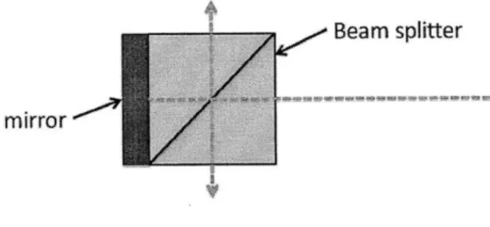
We developed a bi-directional laser with small form factor to use during testing. This component utilized a half mirror (beam splitter) as well as a regular mirror. Components were assembled and aligned with a rapid prototyped part.

Beam splitter

mirror

II -31: Bi directional low form factor laser

Labview realtime software was used to control the system. This software was implemented on a compact RIO (cRIO) that utilized motor driver modules (to drive the motors and read encoder

information as well as to drive the wire coils) as well as an analog input module (to get position information from the PSDs). The software allowed for the operator to choose between a 'driving' and an 'auto-alignment' mode.

Fig. 11-32 shows a CAD model of the outer robot.

Halbach arrays

Harmomic drive motors

Lorentz coils

End effector mockup

II -32: CAD model of functional prototype

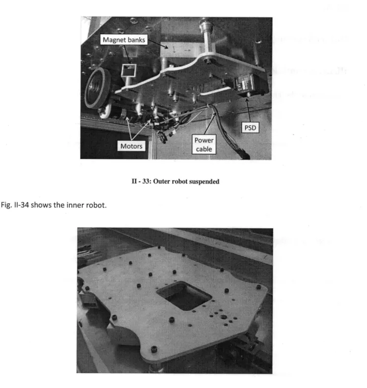
Fig. 11-33 shows this outer robot suspended upside down by its magnet banks.

1 - 33: Outer robot suspended

Fig. 11-34 shows the inner robot.

II -34: Inner robot

This prototype was successfully able to demonstrate required functionality for the fastener installation procedure.

II. Modeling

111.1. Full system model

111.1.1. Assumptions

Fig. Ill-1 shows the inner and outer robots mated with one another across the skin.

III -1: Inner and outer robots across skin

We treat these robots as rigid bodies, modeled as shown in Fig. 111-2. Note that the inner robot has contacts with the skin at the front and rear while the outer robot only contacts the skin at the front wheel. The rear section of the outer robot is constrained along a plane. Additionally, we impose a no-slip condition at the rear wheel -this results in a nonholonomic constraint for the outer robot.

p Inner robot

rigid body

Center of mass

cons raint

We start by examining a free body diagram of the outer robot. The dynamic equations for the outer robot are very similar to those for the inner robot. The forces acting on the outer robot are (1) reaction forces from the skin, (2) magnet forces, (3) torque due to the motor, (4) dissipation terms due to friction and eddy current damping, (5) gravity and, (6) Lorentz forces due to coils.

The state of the robotic system is given by the following:

i -o X, = .1' ,X = ."(O11 yi Oi

A,

-00

Yd

III - 3: Definition of Xd, Yd and Od

X, and X. are the position of the inner and outer robots respectively, their derivative is velocity. Xd is the differential position between the robots. For use in dynamic equations, we define Xd =Xi -X 0 .

(111-2) IF _{= ma,}

EF, _{= ma,}

COM = ICOM

The challenge here is in finding the forces on the system. The forces on the outer robot are given as:

2F.=CO(X,X)-XF-,

=Co(

XdX)-D

-Do,(k VR, (XX

-, Lxx(Xd)y Lyx(X )+Fmotorx

i,- L, (Xdiy Lyy(Xd

)+Fmotor-ix . LXO(Xd _'y .L9(Xd ) + lo-O

And the forces on the inner robot are given as:

-Fi=Cix(XdX)-Dix(Xd,k)+VR,(Xd + , AxL(Xd)+yLyx(Xd)

F;i =Cy(Xd,)-Di,(Xdk)+VRy(Xd)±x-L,,(Xd)+iyL,,(Xd)

x zi =Co( X,k)-DiO(Xd, )+VR(Xd ) x ,4(LXOd)+y -Ly(Xd)

Explanation of terms. Cox (Xd ,I ) is the rolling friction term. This term is dependent on

R,

of the reaction forces on the outer robot (which are in turn a function of Xd ). The velocity of a (passive)

wheel is given by

Vwheel VCOM ± X rOM -wheel

where vCOM - io,94)

(111-5)

And the rolling friction force from a wheel traveling at said velocity can be expressed as

-R

-C.

IVwel

11

Where, for example, the x component of force is found from

Ir

=

Coo(Xd,k)-Do

(k)-VRO(Xd)-(111-3)

-R -C

(|||_7)

[

vwheel

Summing these forces over all passive wheels (2 for the outer robot and 4 for the inner robot) gives C.

D0. (X)is the term dealing with eddy current damping. We assume that eddy damping is a linear

function of velocity. Later we justify this assumption.

VR, (X) Is the term for variable reluctance force between paired magnets (the forces between a magnet on the inner robot and its corresponding magnet on the outer robot). This expression is highly nonlinear.

Fntor x is the motor force acting on the chassis. Note that due to the low inertia of the wheels relative to the chassis, the motor is modeled as a pure force source acting on the chassis.

L, (Xd)is the Lorentz force term due to the coils in the system. For our system, the Lorentz force is

only used when the robots are close to one another; in this case we assume the expression Ly (Xd) is

constant. Note the relationship between the expressions for force on the inner and outer robot: variable reluctance and Lorentz force terms are equal and opposite (as they act between the robots).

Eddy damping and coulomb friction terms are of approximately the same form.

111.1.2. Magnetic forces

We start by modeling the permanent magnets using the magnetic charge model. This is a common approach to this type of problem [4].

III -4: Magnetic charge model

This model approximates a permanent magnet by a pair of surfaces (located at the poles of the magnet) with some density of magnetic charge. For a magnet with magnetization Mi, the surface charge can be found by looking at the change in. magnetization across a boundary.

(111-8) o-,, = -n -yp (M - M )

Free space has no magnetization, so

(111-9)

Usm = PoM

Manufacturers

Magnetization

supply data on a magnet's (BH) max, a measure of the potential energy in a magnet.

at saturation can be related to (BH) through

-(BH) = pMsa

ma

2

We assume the magnet is operating near saturation and use this value to find the magnetic surface charge. In addition, we assume the surface charge is uniform over the magnet pole surfaces.

An analytical solution for the fields of a trapezoidal permanent magnet assumed to have uniform surface magnetic charge density is found in [4]. We assume linearity of the neodymium permanent magnets

and apply superposition to find the field due to a pair of halbach arrays. Fig. 111-5 shows the fields due to a single magnet and those due to a Halbach array.

IH - 5: Fields due to a single magnet (left) and Halbach array (right)

When the field as a function of position is known, it is possible to determine the force and torque on an arbitrary volume in space using Maxwell's stress tensor. To find the forces on the robots, we chose a volume surrounding one Halbach array as shown in Fig. 111-6.

Evaluate field at surface

..

....

.

....

...

III - 6: Evaluating field at some surface surrounding one Halbach array

The surface surrounding this volume was discretized and the field was evaluated at each of these locations. Maxwell's stress tensor about any surface is given as:

P H 2-H _{H2 -H 2)} 2 pH_1H 2

pH

H

E(H

-H)

2

Where the subscript on the field refers to the magnitude of field intensity in that direction. That is, H, is the magnitude of field strength in the x direction. The force on any surface is given by the surface

integral:

uH

H

,uH

H

f,

= fTinjdA

(111-12)

Where T is the ijth entry of Maxwell's stress tensor and nj is±, giving the direction of the normal from

that surface outwards. For example, to find the force in the y direction on a differential surface element parallel to the yz plane where the interior of the volume is larger in x than the element, one would evaluate

-pHH

dA

This method gives us forces and torques as a function of relative displacement and orientation of a pair of Halbach arrays of any strength (this is essentially a FEA software solution built from scratch). The resultant force and torque data was fit to a high order polynomial curve. Approximate magnet force data was taken from the curve fit in practice to speed computation in simulations (as expected, calculating a value from a polynomial fit turned out to be much faster than generating and discretizing a surface, evaluating fields, finding the stress tensor and computing a numerical surface integral). Forces obtained in this method did a reasonably good job of matching the magnitudes of those found experimentally. They did a very good job of scaling similarly to experimental results.

Experimental magnet force measurements were taken with an Admet machine able to vary displacement while recording data. A single axis load cell was used to get force information. The setup

Magnetbank

Force in normal direction measured

III -7: Normal force measurement setup

Data was taken for magnet banks of different strengths, as shown. We were unable to take full six axis force measurements. We instead use these uni-axial force measurements as a way of verifying the

analytical approach we chose.

III -8: Normal force measurements for two different grades of magnets

This data was matched to that obtained analytically as described in the previous section.

III -9: Comparison of simulation to experimental results. Assumptions in magnetic charge density were

scaled in simulation to better match experimental data

It should be noted that the data shown in Fig. 111-9 was scaled to match experimental results. Although the magnets used were grade N50 (according the manufacturer), the data only matched well when we ran the analysis assuming that the magnets were grade N35. Fortunately, the data scaled very well as a function of position. In practice, we suggest taking a single force measurement from a pair of magnets, and using that information to select the 'assumed grade' of the magnet when performing this type of analysis. We believe that using 'assumed grade' in simulations will yield accurate force and torque data; this allows the engineer to explore the effects of a variety of magnet configurations and locations in simulation.

Code used to compute force and torque data can be found in APPENDIX A. Fig. 111-10 shows an example of restoring force as a function of inner / outer robot misalignment generated by this code.

Inner / outer robot misalignment (m)

III -10: Restoring force as a function of inner / outer robot misalignment

The simulation shows results as expected. For small relative displacement of the inner and outer robot, the restoring force is small. This restoring force increases monotonically as the displacement between the robot pair increases, until some point in which its magnitude begins to drop off. Additionally, for small misalignment, the restoring force can be linearized. This plot shows the resultant misalignment force for the case when yd and 0_{d are zero. For Yd # 0, we would expect a similarly shaped plot, but}

with reduced magnitude.

111.1.3. Eddy damping

Maxwell's equations state that a changing magnetic field through a surface induces a proportional voltage through a line around that surface.

S-

B.dA

E

-dl

aA _S

When that surface is in a conductive medium, this voltage creates a current. This current interacts with magnetic fields in the system to oppose the original change in magnetic field. When the change in magnetic field is due to a moving magnet, this is manifested by a force that opposes the motion of the magnet. This results in a 'damping' force felt by a moving magnet.

Eddy current damping is a significant factor in this system due to the high magnetic fields generated by

the neodymium magnets as well as the proximity to a large conductive surface (the aluminum skin). This force is often modeled as scaling linearly with respect to velocity. We assume that our system operates in a regime where this is the case, and tested our assumption with an experiment, described here.

We used the passive inner robot from the prototype and ran two sets of trials. In the first set of trials the inner robot was operating on a conductive aluminum skin. In the second set of trials it operated on a non-conductive acrylic sheet. In all trials the robot was accelerated to some velocity (not consistent

between trials) and released. An accelerometer attached to the robot recorder acceleration data as the robot slowed; integrating this data gives velocity information.

If eddy current damping did in fact act linearly with respect to velocity, the dynamic equations of motion

of the system are given as:

m, = -bV - cN _{mx -M- cN(Ill-15)}

mv = -bv - cN

Where b is the coefficient of eddy damping, c is the coefficient of rolling friction, and N is the normal force from the skin (equivalent to mg: the product of the mass of the robot and the acceleration due to gravity). Solving these equations is straightforward: