Computational modeling of trabecular bone in lower extremity injuries due to impact

Computational Modeling of Trabecular Bone in

ARCHNES

Lower Extremity Injuries due to Impac

OF TECHNOLOGY

by

JUN

2

5 2013

Wendy Pino

B.S., Aeronautics and Astronautics -Le9B/\I.

Massachusetts Institute of Technology, Cambridge (2011)

Submitted to the Department of Mechanical Engineering

in partial fulfillment of the requirements for the degree of

Master of Science in Mechanical Engineering

at the

MASSACHUSETTS INSTITUTE OF TECHNOLOGY

June 2013

©

Massachusetts Institute of Technology 2013. All rights reserved.

Author ... ... .. ...

Department of Mechanical Engineering

May ,. 2013

Certified by...

Rad*l A. Rafovifzky

Professor of Aeronautics and Astronautics

Thesis Supervisor

Certified by...

Lorna J. Gibson

Professor of Mechanical and Materials Science Engineering

4 . ,4' is1 der

Accepted by ...

E

Cavid E. Hardt

Computational Modeling of Trabecular Bone in Lower

Extremity Injuries due to Impact

by

Wendy Pino

Submitted to the Department of Mechanical Engineering on May 10, 2013, in partial fulfillment of the

requirements for the degree of

Master of Science in Mechanical Engineering

Abstract

Lower extremity injuries resulting from improvised explosive devices (IEDs) pose a serious threat to the safety of military troops. Reports from Operation Iraqi Freedom and Operation Enduring Freedom identify IEDs as the cause for a substantial number of lower extremity bone fractures. The Army Research Laboratory (ARL) concen-trates part of its research efforts into better understanding impact related injuries. Despite a significant number of articles on bone mechanical behavior, only a few con-sider high strain rates. In collaboration with ARL, we propose in this thesis to capture

via an in silico approach the dynamic and quasi-static responses of the trabecular

bone. To achieve this goal, we conducted large scale parallel finite element simu-lations on biofidelic and biomimetic morphological models of trabecular bone. The biofidelic model was developed using an image-based tetrahedral meshing approach on pCT images, courteously provided by Niebur's group at Notre Dame University, of a human femural sample. The biomimetic model was developed from an analytical model proposed by Wang and Cutifno [50] for a periodic unit cell. For the solid part of the trabecular, a visco-elastic visco-plastic constitutive model developed by Socrate's group [15] for cortical bone was applied. For the dynamic simulations, the effect of strain rate on the response of the bone microstructure was investigated and com-pared to published experimental results. We observed a structural softening on the stress-strain curve which takes its origins from the buckling that appears within the spongious trabeculae structure. Finally we included fracture in our dynamic simula-tions using the discontinuous Galerkin method developed by Radovitzky's group

[37]

Thesis Supervisor: Radil A. Radovitzky

Acknowledgments

I would like to express the deepest gratitude to my research advisor, Prof. Radl

Radovitzky, for giving me the opportunity to take part in the exciting and meaningful research that his group is conducting. I am extremely grateful for his invaluable guidance, support and understanding. I would like to thank him for sharing his wealth of knowledge while helping me work through the tough problems that arose and for sharing his genuine enjoyment of research. Radl, gracias por su interes en mi bienestar y por hacerme sentir como en casa.

My sincere thanks go to Dr. Aurelie Jean for her constant encouragement and

moti-vation. I would like to thank her for caring about my success and investing so much time in teaching me new skills. Her insight has been extremely valuable to me. I would also like to thank her for helping me make improvements to this thesis. She is someone I aspire to be more like in my career and in life. I know that she will make a wonderful professor.

I would also like to thank the members of the RR group, including Abiy Tasissa,

Adrian Rosolen, Andrew Seagraves, Brandon Talamini, Gauthier Becker, Lei Qiao, Martin Hautefeuille, Michael Tupek, and Michelle Nyein, for their friendship, support,

and interest in my academic progress.

Additionally, I would like to express my gratitude towards Dr. Simona Socrate for providing the constitutive model implemented in this study and for her hands-on approach to investigating problems with me. I would also like to thank Prof. Glen Niebur from the University of Notre Dame for generously providing images of tra-becular bone which were used to create our model. For their contributions, I am extremely appreciative.

I am also thankful for the financial support provided by the Army Research

Labora-tory (ARL) and the Institute for Soldier Nanotechnologies (ISN). From ARL, I would like to thank Dr. Reuben Kraft for his efforts during our collaboration.

I would like to thank Samuel Dyar for his help and encouragement every step of the

way. For his love and advice, I am deeply grateful. Lastly, and above all, I would like to thank my parents for taking the risks and making the sacrifices that have made this opportunity a reality. This would not be possible without their immense love and support.

Contents

1 Introduction

1.1 M otivation. . . . .

1.2 Advanced Computational Mechanics Capabilities for

A pplications . . . .

1.3 O bjectives . . . .

1.4 O utline . . . .

2 Trabecular Bone Properties

2.1 Biological Hierarchical Structure of Trabecular Bone . 2.1.1 Observation of Microstructure . . . .

2.1.2 Characterization of Microstructure . . . .

2.2 Mechanical Behavior of Trabecular Bone . . . .

2.2.1 Most Relevant Characteristics . . . .

2.2.2 Relative Density and Anisotropy . . . .

2.2.3 Strain Rate Effect on Mechanical Behavior . .

2.2.4 Fracture Mechanism . . . .

2.2.5 Quasi-static Experimental Results . . . .

19 19 Bone Fracture . . . . 20 . . . . 21 . . . . 21 23 . . . . 23 . . . . 23 . . . . 24 . . . . 25 . . . . 25 . . . . 26 . . . . 28 . . . . 29 . . . . 30 3 Morphological Modeling of Trabecular Bone Microstructure

3.1 Periodic Biomimetic Microstructures . . . .

3.1.1 State of A rt . . . .

3.1.2 Geometrical Structure of a Single Unit Cell . . . . 3.1.3 Geometrical Structure of a Tessellation Unit Cell . . . .

33 33 33

34

3.1.4 Geometrical Structure of the Tessellation . . . . 36

3.1.5 Trabecular Dimensions . . . . 38

3.2 Image-based Biofidelic Microstructure . . . . 40

3.2.1 M eshing Procedure . . . . 41

4 Material Behavior Modeling of Trabecular Bone 49 4.1 Previous Models in Literature . . . . 49

4.2 Constitutive Equations . . . . 50

4.3 Implementation in Summit . . . . 52

5 Modeling Framework 53 5.1 Computational Framework . . . . 53

5.2 Finite Deformation Numerical Formulation . . . . 53

5.3 Discontinuous Galerkin . . . . 55

5.4 Solver: Newmark Scheme . . . . 55

6 Numerical Simulation of Quasi-Static Test 57 6.1 Numerical Method: Dynamic Relaxation Solver . . . . 57

6.1.1 Implementation in Summit . . . . 57

6.1.2 Example: Convergence of Prismatic Bar . . . . 60

6.2 Quasi-Static Simulation of Biomimetic Trabecular Bone . . . . 63

6.3 Quasi-Static Simulation of Biofidelic Trabecular Bone . . . . 65

6.4 D iscussion . . . . 68

7 Numerical Simulation of Dynamic Test 69 7.1 Numerical Method: Parallel Design for Periodic Structures in Summit 69 7.2 Dynamic Simulation of Biomimetic Trabecular Bone . . . . 71

7.3 Dynamic Simulation of Biofidelic Trabecular Bone . . . . 75

7.3.1 Trabecular Bone Sample A . . . . 75

7.3.2 Trabecular Bone Sample B . . . . 75

7.4 Dynamic Fracture Simulations using Discontinuous Galerkin . . . . . 81

7.4.2 Fracture Simulation of Biofidelic Trabecular Bone . . . . 81

7.5 D iscussion . . . . 85

8 Conclusions 87 8.1 D iscussion . . . . 87

8.2 Recommendations for Future Work . . . . 89

8.2.1 Quasi-static Fracture Simulation . . . . 89

8.2.2 Large Scale Bone Modeling . . . . 89

List of Figures

2-1 Structure of cortical bone (a) 3D Sketch of cortical bone, (b) Haver-sian system cut, (c) HaverHaver-sian system photomicrograph, Fridez P. Mod lisation de l'adaptation osseuse externe. PhD thesis, In Physics

Department, EPFL, Lausanne, 1996 . . . . 25

2-2 Scanning electron micrograph of low density (a) rod-like trabecular bone and high density (b) plate-like trabecular bone taken from the femoral head of a human specimen [9]. . . . . 26

2-3 Plot of compressive strength vs density of trabecular bone as presented by [10]. The plots show earlier (a) and later (b) studies conducted hu-man bone specimens, unless specified otherwise. Relative compressive strengths are normalized by oy, = 182 MPa and relative densities are normalized by ps = 1800 kg/m. . . . . 28

2-4 Stress results found in literature for quasi-static experimental tests on trabecular bone samples. . . . . 30

3-1 Bottom part of Cuitifio unit . . . . 35

3-2 Single Cuitifio unit . . . . 35

3-3 Two Cuitifno unit cells joined together. . . . . 36

3-4 Tessellation unit cell containing 73,121 tetrahedral elements and 12,634 nodes, generated using gmsh. . . . . 37

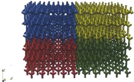
3-5 Tessellation based on the Cuitifio model consisting of 564,104 tetrahe-dral elements. Each color represents a different processor. . . . . 38

3-6 Slice of pCT viewed in ImageJ [42] consisting of 384 x 384 pixels and

representing an 8mm x 8mm cross-sectional area. . . . . 38

3-7 Marching cube used for mesh triangulation placed between two slices

of images, as shown by Lorensen and Cline [22]. . . . . 41

3-8 Triangulated cubes based on label combinations taken from each vertex

of the cube, as shown by Lorensen and Cline [22]. . . . . 42

3-9 Layered stacks of segmented binary images of trabecular bone taken

from pCT and imported in AMIRA. Each slice consists of 384x384x1 pixels. There are 371 slices in the z direction. . . . . 43

3-10 Trabecular bone mesh after processing pCT images in Amira and then

meshing in Ansys to create a mesh consisting of 2, 379, 141 linear tetra-hedral elem ents. . . . . 45

3-11 Trabecular bone meshes for sample A and sample B. . . . . 46

3-12 Zoomed in image of part of the trabecular bone mesh in the same

vicinity for meshes created using different processes. The mesh that results from AMIRA and Ansys is a higher quality mesh. . . . . 47 4-1 Stress-strain solid curve fits from the Johnson constitutive model

com-pared with data points from the McElhaney experiment. [15] . . . . . 50

4-2 Constitutive model schematic representing visco-elastic, visco-plastic bone from [15] . . . . 51 6-1 Spatial distribution of the displacement field along the z direction

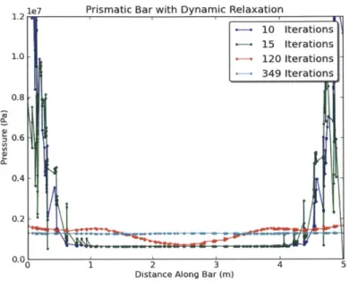
af-ter convergence of DR solver, for a displacement prescribed at both extremities of the prismatic bar along the z direction. . . . . 60 6-2 Evolution of the pressure as a function of the position along the

pris-matic bar at different iterations of the DR solver: the response reaches static equilibrium as the number of DR iterations increases. . . . . . 61 6-3 Evolution of the displacement as a function of the position along the

prismatic bar at different iterations of the DR solver: the response reaches static equilibrium as the number of DR iterations increases. . 62

6-4 Evolution of pressure as a function of the position along the prismatic bar after the first time step and for different tolerance values in the D R solver. . . . . 62 6-5 Stress gradient result for a tessellation under compression using

dy-namic relaxation and the Neo-Hookean material model. . . . . 63

6-6 Force vs. displacement for a 1x1x1 single tessellation unit in

compres-sion using the Neo-Hookean material model. . . . . 64

6-7 Force vs. displacement for a 1x1x1 single tessellation unit in

compres-sion using the cortical material model. . . . . 64

6-8 Dynamic relaxation convergence study for sample A for both the Neo-Hookean and the cortical material model. . . . . 65 6-9 Dynamic relaxation convergence study for sample A for both the

Neo-Hookean and the cortical material model. . . . . 66 6-10 Evolution of the stress in the z direction o-2, as a function of the strain

in the z direction E2, for a quasi-static test conducted on sample A of the biofidelic model using the cortical bone material. . . . . 67 6-11 Evolution of the stress o-2 for sample A under compression with a

maximum displacement of 5.025x10-6 using dynamic relaxation and the cortical material model. . . . . 67 7-1 Representation of Message Passing Interface (MPI) application setup

for an 8 processor simulation with a tessellated unit cube. Processors are numbered left to right in the x-direction, then in the y-direction, and the z-direction. . . . . 71 7-2 Mesh of biomimetic bone tessellation comprised of 1,440 tessellation

units that corresponds to a total sample size of 11.7 mm x 11.2 mm x

11.1 mm. The current image is a partial view of the entire structure,

7-3 _{Spatial distribution of the stress components azz in the biomimetic}

bone microstructure. The current image is a partial view of the en-tire structure, displaying 20 of the 72 processors using Paraview and

demonstrating displacement. . . . . 73

7-4 Evolution of the stress component ozz as a function of the strain com-ponent czz from the dynamic simulation conducted on the biomimetic bone tessellation with an initial velocity of 10 m/s applied to both extremities of the structure along the z-axis. . . . . 74

7-5 Evolution of the stress component ozz as a function of the strain com-ponent czz from the dynamic simulation conducted on sample A at 10 m/s in loading directions x, y, and z. . . . . 76 7-6 Spatial distribution of the stress component along specific loading

di-rections x (a), y (b), and z (c) within sample A of the biofidelic mi-crostructure. . . . . 76

7-7 Simulation result showing uCT sample B under dynamic compression

with 10 m/s applied to the z extremities at time 2.89 x 10-5 seconds. 77 7-8 Evolution of stress azz as a function of strain ezz for sample B CT

simulations run at different strain rates. . . . . 78 7-9 Evolution of stress orzz as a function of strain ezz for pCT simulation on

sample B with a strain rate of 330/s demonstrating post-yield softening

due to buckling. . . . . 79

7-10 Spatial distribution of stresses uz2 from dynamic simulation on

biofi-delic sample B with a velocity boundary condition of 1.10 m/s. ... 80 7-11 Spatial distribution of the stress component Uzz within the trusses of

one single unit-cell of the biomimetic model of trabecular bone after

10 and 30 time steps of a dynamic simulation with DG. The opened

interface elements characterizing cracks are highlighted in green in the contour plots. . . . . 82

7-12 Evolution of stress ozz with respect to strain Ezz for a dynamic

simu-lation on sample A using both continuous Galerkin (CG) and discon-tinuous Galerkin (DG) in order to compare the effect of allowing for discontinuities. . . . . 83 7-13 Spatial distribution of stresses oz for a DG dynamic simulation of

sample A under compression at a time of 2.531x10-6 s. . . . . 84 7-14 Visualization of the fracture surfaces within sample A of trabecular

bone for a compressive dynamic simulation at time 2.531x10-6 S. In-terfaces with a minimal separation of 3.3x10-6 between elements are

highlighted in red. . . . . 84

8-1 Single time-step showing several iterations of dynamic relaxation up to convergence, applied to sample A with 67,114 tetrahedral elements prior to m esh scaling. . . . . 90 8-2 Four time-steps showing several iterations of dynamic relaxation up

to convergence, applied to sample A with 67,114 tetrahedral elements prior to mesh scaling. The legend indicated number of interface ele-ment openings and average opening distance in meters. . . . . 91 8-3 Evolution of stress o-z for the converged solution of a prismatic bar

run with dynamic relaxation and DG. . . . . 91

8-4 Dynamic simulation of a full tibia bone consisting of 145, 669 tetrahe-dral elements and 1, 531, 768 nodes. . . . . 92 8-5 Dynamic simulation on full tibia mesh with fracture. Bulk elements

are shown in gray and fractured cohesive elements are shown in red. . 93 A-1 Full assembly of three layers of processors showing the spatial

relation-ship between one another. . . . . 96

List of Tables

2.1 Example Material Properties for Bone, Kraft et. al [21] . . . . 27

2.2 Data from trabecular bone extracted from experiment curves in liter-ature showing strain rate i, stiffness, and maximum stress o-. Data for bone volume to total volume percentage, sample length, sample di-ameter, species, and anatomical origin of specimen were given in each source. For the stiffness, these results give an average stiffness of about

0.9 GPa with a standard deviation of 0.398 GPa. . . . . 31

4.1 Material properties specified by the user to describe trabecular bone, calibrated with McElhaney experiments [15]. . . . . 52 7.1 Data from trabecular bone simulations conducted on sample B showing

strain rate i, stiffness, maximum stress o-, bone volume to total volume percentage, sample length, and sample diameter. . . . . 78

Chapter 1

Introduction

1.1

Motivation

Improvised Explosive Devices, known as IEDs, present a dangerous threat to the safety of military troops. In the case known as an underbelly blast, an improvised explosive device is detonated under a military vehicle. This results in a high amplitude short duration pressure wave [26] which propagates through the floor of the vehicle and impacts the foot and lower leg region of the occupant. The impact can sometimes incapacitate a soldier instantaneously [26].

These anti-vehicular mines hinder the ability of the military to react quickly. They diminish the strength of troops and even lower morale. Explosive devices not only injure soldiers, but also block access paths for help to arrive and increase costs asso-ciated with medical air transportation [38].

A study of the injuries sustained by soldiers in Operation Iraqi Freedom (OIF) and

Operation Enduring Freedom (OEF) reported a total of 3, 575 extremity combat injuries between October 2001 and January 2005. 75% of extremity injuries to soldiers in OIF and OEF were caused by improvised explosive devices [32]. 26% of these

injuries involved bone fractures, with half of the fractures sustained in the lower extremities, most commonly in the tibia and the fibula.

These circumstances are costly, difficult, and sometimes impossible to replicate

ex-perimentally. Therefore, it would be valuable to be able to predict the fracture of bone using 3D finite element simulations.

1.2

Advanced Computational Mechanics

Capabil-ities for Bone Fracture Applications

Trabecular bone is an active area of research. It was first investigated in the 1847, but then more consistently in the 1960s. Since then, research in this area has been steadily increasing to over 700 publications in the last year alone. A search (on pubmed.gov) yielded 11,105 papers about trabecular bone. Only about 5% of those papers dealt with numerical studies. An even smaller amount, 1.03%, incorporated bone fracture or crack propagation into their studies and 0.8% analyzed fracture in 3D. There were no publications found that utilized Message Passing Interface (MPI) or discontinuous Galerkin (DG). Despite the small number of fracture publications, many sources [12]

[43] [26] stress the importance of bone analysis in fracture related cases, both for blast

scenarios and for falls experienced by the elderly.

Part of the reason there is a shortage of numerical simulations is because the begin-nings of ongoing trabecular bone research coincide with the beginning of discontinuous Galerkin finite elements and commercially available parallel computers.

Finite element development began with Alexander Hrennikoff and Richard Courant [34] in the early 1940s. They both used mesh discretization and the idea of elements. In 1947, Olgierd Zienkiewicz consolidated the various methods into finite elements

[44]. Discontinuous Galerkin methods were not developed until 20 years later. Parallel computing was introduced in the mid 1950s. However, it wasn't until April 1958 that it was considered for use in finite element calculations [52].

This purpose of this study is to understand the fracture of trabecular microstruc-tures, but also to make use of computational advances by incorporating MPI and DG

finite elements. Therefore, there are interests in both the bone application and the computational approach.

1.3

Objectives

The objective of this study is to model the mechanical response of trabecular bone at high strain rates. Towards that goal, a material model that can accurately represent bone is included in the model. Meshes generated from real bone specimens and from idealized geometries serve as samples for analysis. The focus is to look at the stiffness, yield, and fracture response of the samples.

Experiments can be expensive, limited in quantity, and sometimes difficult to repro-duce for explosive cases. Therefore, fracture is more feasible to model than to study experimentally. Proper modeling of trabecular bone behavior in this study will serve as a tool for further investigation and for design of protective gear.

1.4

Outline

The consequences of lower extremity injuries serve to highlight the importance of this study. This first section established goals, both mechanical and numerical, that need to be attained in order to better understand the response of bone tissue. In the next section, bone characteristics are described in detail, first from a biological point of view and then from a mechanical point of view.

Then, morphological modeling of bone is explained. For one sample, a biofidelic mesh was generated from images of real trabecular bone. For another sample, an idealized microstructure was created based on the Cuitifno geometry

[50].

Lastly, static and dynamic simulations using a finite element code developed within the Radovitzky group

[37]

The resulting behavior, including plasticity, buckling, and fracture are analyzed and discussed.

Chapter 2

Trabecular Bone Properties

2.1

Biological Hierarchical Structure of

Trabecu-lar Bone

2.1.1

Observation of Microstructure

Significant efforts have been made to study and identify the key geometrical and mechanical features of bone. It is known that length and thickness of trabeculae have a strong impact on the overall macroscopic behavior. These dimensions are quantified through observations and measurements of medical images. The most popular techniques include various forms of computed tomography such as peripheral high-resolution computed tomography (HR-pQCT) and micro-computed tomography (puCT)[6] [41] [13] [29]. Magnetic resonance (MR) and Scanning Electron Microscopy are among other methods that have been used[27] [51]. The methods mentioned have been applied in either in vivo or post-mortem cases [24].

2.1.2

Characterization of Microstructure

In order to fully model underbelly blast problems, it is important to understand the structural characteristics of bone. By understanding its properties and constitutive behavior, we can create more accurate models to numerically simulate events that happen in combat.

The structure of bone allows it to function as a high strength, low weight support mechanism. Bone consists of a hard outer layer, known as the cortical, and a porous inner core known as the trabecular.

Cortical bone tissue can be considered a composite material and is known for its heirarchical structure. It is composed of hydroxyapatite, collagen, proteoglycans, noncollagenous proteins and water [5]. At the microscopic level, cortical bone is composed of Haversian canals that are aligned longitudinally along the bone. These canals are connected transversely by Volkmanns canals with capillaries and nerves. Cylindrical lamellae surround the Haversian canals to create osteons. Cement lines surround each osteon in order to separate Haversian canals from the interstitial bone

[5] [1]. These microstructures are densely packed. In fact, cortical bone has about 5-10% porosity [5].

Bone contains a porous inner core consisting of trabecular tissue. This is also known as cancellous bone. At the microscale, trabecular bone is composed of individual trabeculae struts in three dimensional space which form an open cellular structure

[9]. This cellular structure contains interconnected rods and plates at a variety of

angles. Unlike the densely packed cortical bone, trabecular bone has a porosity of

50-95% [5]. Figure 2-1 shows the dense cortical surrounding the open, sponge-like

trabecular architecture.

Trabecular bone properties can vary with age and with anatomical location. The orientations and sizes of the cells develop according the directions and magnitudes of the loads it needs to support [9] [19].

(b)

Figure 2-1: Structure of cortical bone (a) 3D Sketch of cortical bone, (b) Haver-sian system cut, (c) HaverHaver-sian system photomicrograph, Fridez P. Modelisation de l'adaptation osseuse externe. PhD thesis, In Physics Department, EPFL, Lausanne,

1996

At different anatomical locations, bone will have cortical and trabecular sections, however the trabecular composition will vary as stated previously. Therefore, the porous interconnected architecture of trabecular bone is optimized to support heavy loads while maintaining a low weight. With age, individual trabeculae also become thinner, thus altering its material properties [43]. Trabecular bone is heterogeneous, in the sense that volume fraction, moduli, and strength can vary spatially across a single bone specimen [19]. For this reason, it is desirable to understand the spatial distribution of localized stresses at the bone microscale in addition to the global stress response.

2.2

Mechanical Behavior of Trabecular Bone

2.2.1

Most Relevant Characteristics

Trabecular bone is an open cellular material composed of interconnected rods and plates, as visible in Figure 2-2. Its most important characteristic is relative density, or the fraction of solid to total volumetric space. Cell size plays a lesser role in

determining mechanical properties. Nevertheless, cell shape is important because it captures the anisotropy of bone. Topology is yet another important characteristic. The 3D open cell structure of the trabecular provides information about edges, faces, and connectivities that in turn affect mechanical properties [9]. Sample material properties can be seen in Table 2.1. Bone has been characterized as anisotropic, visco-elastic, and visco-plastic. Trabecular bone only makes up 15-20% of the entire bone material. However, its lightweight cellular structure provides important shock

absorbing capabilities and added strength [39]. The microstructure of trabecular

bone can vary based on anatomical location. It can develop to support the loads encountered by the human body and by doing so, it can establish a direction along which stiffness and strength are greatest [19].

(a) (b)

Figure 2-2: Scanning electron micrograph of low density (a) rod-like trabecular bone and high density (b) plate-like trabecular bone taken from the femoral head of a human specimen [9].

2.2.2

Relative Density and Anisotropy

One of bone's most important characteristics is the ratio of the density of trabecular bone to the desity of solid bone. Important values such as Young's modulus and yield stress, are dependent on relative density. As seen in Figure 2-3 relative density can

Bone Type Material Property Cortical E = 19.0 GPa v = 0.3 p = 1810kg/m 3 c= 132MPa Trabecular E 300 MPa v = 0.45 p = 600kg/m 3 ac = 1.5MPa

Table 2.1: Example Material Properties for Bone, Kraft et. al [21]

have a strong effect on strength. Several attempts have been made to develop power laws to characterize the relationship between density and modulus. One analysis, by Lotz et al. [23], formulated some relationships describing the elastic modulus and critical stress for varying levels of bone density p shown in Equations 2.1-2.4:

E(MPa) = 1904 p1

.64 axial direction

E(MPa) = 1157 p1

.78 transverse direction

0c(MPa) = 40.8 p1_.89 _{axial direction}

ac(MPa) = 21.4 -p137 _{transverse direction}

(2.1) (2.2)

(2.3)

(2.4)

It is important to note that the relationships developed by Lotz are different for the axial and transverse directions, thereby capturing the anisotropy in bone.

Another quantifiable property used to characterize bone is ash fraction. Ash fraction allows you to account for bone mineral content, a property which influences mechan-ical behavior. [14]. They note that many models do not account for the difference between bone volume fraction B and ash fraction a, and present a way to relate

p =B (1.41 + 1.29a) (2.5)

TV

It is important to note that although these relationships can characterize mechanical properties of bone, they do not take into account the effect of microstructural architec-ture. Therefore, a correlation between trabecular microstructure and macrostructure would provide a more rigorous understanding of the mechanical behavior.

102 103 102 1?.

~ W.I~. eh e.ins-We41 md 5" (19574

F,.,.. and 4.6i. Fesnu. a.4 t". Cr ier aves (1077) aCarern d Haves f 1677

rbial ylabass Mist

o Hgy.4 nd Cat. (416) 00 anCarterONff61 On

soin ta C.i Snia o i dlS4)

W.*w .n1 baml~ 7165 - Wff. am Chtalmers 411161 G':

0.1 tat ia' Ca I.~

S ., ILnr0X L OKN 0 0 + , 0.01 0.10*4 *c4* *ai JO c4k ** Or 1' 22 0.001 0.001 0.01 0.1 1 0.01 0.11

Relative density, jp 'p Reltive defrsitV. prf p

(a) (b)

Figure 2-3: Plot of compressive strength vs density of trabecular bone as presented

by [10]. The plots show earlier (a) and later (b) studies conducted human bone specimens, unless specified otherwise. Relative compressive strengths are normalized

by aus 182 MPa and relative densities are normalized by p,8 1800 kg/in3.

2.2.3

Strain Rate Effect on Mechanical Behavior

Bone has been known to exhibit time dependent behavior [19]. Thus, efforts have been made to characterize the response of bone loaded under various strain rates.

While many experiments have been conducted at low strain rates, few have been done at strain rates higher than 10 s-'. One experiment, conducted by McElhaney, used an air gun type setup to apply compressive forces to a trabecular bone specimen. They achieved strain rates of up to 4,000 s1 and captured the stress-strain response curves for bone at different strain rates [25]. Their stress-strain curves showed an increase in bone modulus as strain rate increased. It was also noted that different fracture response were exhibited for the strain rates tested. At strain rates below

1s-', the types of fractures were shear failures and cone failures, whereas at higher

strain rates the fractures were splinters in the longitudinal direction.

In an experiment conducted by Bonfield and Clark, it was also reported that Young's modulus increased with strain rate almost linearly before plateauing at a bounded value [2]. In yet another paper by J.D. Currey, the trend between strain rate and modulus was plotted and it was deduced that by increasing the strain rate 1,000-fold, the Young's modulus increased by 10%.

2.2.4

Fracture Mechanism

Bone fracture can occur due to impact associated with trauma scenarios or due to muscle contraction of fatigued bones in elderly people [5] [19]. Bone has the ability to dissipate energy in order to prevent fracture. This has been associated with its geometrical features, but also with constitutive properties such as visco-plastic flow

[35].

The anisotropy found in bone affects the way in which fracture patterns propa-gate. There is a preferential longitudinal direction along which cracks propagate more smoothly than across transverse cross sections of the bone. It has been found that for angles between 0-50' cracks are smooth, whereas for angles 50-90' cracks are zig-zagged and require a higher fracture energy. Transversely, microstructures in the cortical region, such as cement lines, can divert the direction of crack propagation and even stop it [1]. The anisotropy of bone allows the fracture energy between directions

to change by two orders of magnitude

[35].

2.2.5

Quasi-static Experimental Results

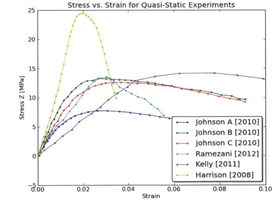
In the literature, several quasi-static experimental results for trabecular bone samples have been documented. The most relevant information including sample origin, di-mension, strain rate, apparent stiffness, and maximum stress have been summarized in Table 2.2. Of the sources that provided stress plots, the data has been visually extracted and plotted together in Figure 2-4 for comparison. The results in the liter-ature give an average stiffness of about 0.9 GPa with a standard deviation of 0.398 GPa. The average maximum strength from the values reported is 15.74 MPa, with a standard deviation of 4.96 MPa.

25 N 20 - 15- 10-5 0

Stress vs. Strain for Quasi-Static Experiments

0 0.02 0.04

Strain

0.06 0.08 0. LO

Figure 2-4: Stress results found in literature for quasi-static experimental tests on

trabecular bone samples.

Johnson A [2010] Johnson B [2010] Johnson C [2010] - -+ Ramezani [2012] . - Kelly [2011] Harrison [2008] 0

Experimental Values for Quasi-Static Tests

Source Stiffness [GPa] Max o [MPa] BV/TV

[%]

Ramezani [2012] 0.027 0.5 13.5 - 10.0 7.0 Human Femoral Head

Johnson Specimen A [2010] 0.01 0.6 7.7 14.4 % 3.773 7.175 Bovine Femur

Johnson Specimen B [2010] 0.01 0.935 13.2 21.0% 3.843 7.263 Bovine Femur

Johnson Specimen C [2010] 0.01 0.75 12.5 26.6 % 3.779 7.275 Bovine Femur

Kelly [2011] 0.0104 0.31 14.2 - 8.0 8.0 Bovine Proximal Tibia

Harrison [2008] 0.001 1.65 24.5 - 10.0 7.0 Ovine L5 Vertebrae

Verhulp Specimen 1 [2008] 0.00017 1.34 24.55 34.1% 5.0 5.35 Bovine Proximal Tibia

Verhulp Specimen 2 [2008] 0.00017 1.24 21.27 31.5% 5.0 5.35 Bovine Proximal Tibia

Verhulp Specimen 3 [2008] 0.00017 1.07 18.27 28.5% 5.0 5.35 Bovine Proximal Tibia

Verhulp Specimen 4 [2008] 0.00017 0.94 14.41 35.6% 5.0 5.35 Bovine Proximal Tibia

Verhulp Specimen 5 [2008] 0.00017 0.73 19.08 34.3% 5.0 5.35 Bovine Proximal Tibia

Verhulp Specimen 6 [2008] 0.00017 1.23 21.83 30.3% 5.0 5.35 Bovine Proximal Tibia

Verhulp Specimen 7 [2008] 0.00017 0.41 10.36 18.4% 5.0 5.35 Bovine Proximal Tibia

Table 2.2: Data from trabecular bone extracted from experiment curves in literature showing strain rate i, stiffness, and maximum stress o. Data for bone volume to total volume percentage, sample length, sample diameter, species, and anatomical origin of specimen were given in each source. For the stiffness, these results give an average stiffness of about 0.9 GPa with a standard deviation of 0.398 GPa.

Chapter 3

Morphological Modeling of

Trabecular Bone Microstructure

3.1

Periodic Biomimetic Microstructures

3.1.1

State of Art

Periodic structures can be used to represent cellular solids [11] and study the be-havior of trabecular at the microscale. By tessellating a design that represents the architecture of trabecular bone, a full network of interconnected trabeculae can be created.

Studying the bone structure at this level of detail will allow us to observe any lo-calized behavior that is not seen at the macroscale. In fact, it has been found that microstructural strains can be up to 2.2 times larger than the continuum strains

[40].

Periodic tessellations of unit cells have been used to represent trabecular bone in several cases. In a study done by Guo and Kim [12], different unit cells were used to represent rod-like and plate-like trabecular sections for the purpose of understanding the effect of bone loss on mechanical response. Another study by Sander [40] used

rectangular open cell and offset rectangular open cell structures to model vertebral trabecular bone. Periodic unit cells were even applied to model cortical bone in addition to trabecular bone [3]. This was done by tessellating square unit cells and varying the porosity by choosing different geometrical configurations to fill the unit square.

I've chosen to assemble and design the meshing for a particular structure studied

by Cuitiio et al. [50] because it has several good qualities. It can be generated by

tessellating a single unit cell, it describes an open cellular structure, and it has been shown to capture anisotropy at different orientations.

3.1.2

Geometrical Structure of a Single Unit Cell

To capture the microstructure of trabecular bone, a unit cell was created inspired by the Cuitifio model using Gmsh [8]. The attributes of the unit cell (angle 0, length 1, and radius r) are specified by the user for added flexibility. By tessellating the unit cell, we created a geometry that represents that of bone.

The cell consists of 4 cylinders which fuse at the origin. The top three cylinders are referred to as struts, and the bottom cylinder is referred to as the handle. To create the unit, I began by creating a point at the origin and considering all other points that will lie on the z = 0 plane. Since there are 3 struts, there will be 3 points on the z=0 plane at the location where the sides of the cylinders meet. These points (2, 6, 7) were created with 120 degrees of separation to fit the three cylinders. Next, I created points (3, 4, 5) that "dip" a little below the z=0 plane. At these points the struts from the top will join with the handle at the bottom.

To completely define the intersection, I created point to establish the height at which the 3 struts fuse. The distance between that point and the origin is labeled by h. To create the handle, the points that lie on the z = 0 plane were extruded in the negative z-direction a distance 1. The base of the handle (10, 11, 12) was duplicated and rotated about the y-axis so that the angle with the z-axis was 0, as requested by

Figure 3-1: Bottom part of Cuitiio unit

the user. This creates the first strut. By rotating the strut by 120 and 240 degrees the last two struts were created. To finish the unit, circular arcs, ellipses, and lines were added to create surfaces which describe the unit volume.

2r

Figure 3-2: Single Cuitinio unit

Once the uniit cell is created, it can be

joined

joined

YX

3.1.3

Geometrical Structure of a Tessellation Unit Cell

As mentioned previously, single unit cells can be combined. A tessellation unit cell, shown in Figure 3-4, is composed of 12 single unit cells. The tessellation unit can be replicated in 3D space to create a open large cellular structure simply by mov-ing it by an established dx, dy, dz distance without needmov-ing rotations or complex

algorithms.

3.1.4

Geometrical Structure of the Tessellation

By simply moving the tessellation unit cell by dx, dy, or dz, an entire block of

tes-sellated material can be created without the need for a complex algorithm. For the tessellation unit chosen, the vector translations below allow us to fill the 3D space

w

z

I

Y

Figure 3-4: Tessellation unit cell containing 73,121 tetrahedral elements and 12,634 nodes, generated using gmsh.

while maintaining connectivity between the units.

dx = [4lsin(O)(sin(7r/6) + 1), 0, 0] (3.1)

dy = [0,4lsin(O)cos(7r/6), 0] (3.2)

dz = [0, 0, 3(21)(1 + cos(O))] (3.3)

(3.4)

The tessellated structure shown in Figure 3-5 contains a tessellation in every processor which is made up of multiple tessellation units. It measures 4.06 mm, 2.84 mm, and

Figure 3-5: Tessellation based on the Cuitifio model consisting of 564,104 tetrahedral elements. Each color represents a different processor.

3.1.5

Trabecular Dimensions

The program which generates the idealized microstructure tessellations takes the ra-dius, length, and angle of unit as inputs. Therefore, it is important to prescribe values which will realistically represent the bone anatomy of our specimen. Individual tra-beculae length has been documented by several sources [43] [40] [281.

Figure 3-6: Slice of pCT viewed in ImageJ [42] consisting of 384 x 384 pixels and representing an 8mm x 8mm cross-sectional area.

and transverse directions are calculated from 2D images of a vertebral bone specimen. They tabulate results for trabeculae dimensions based on age. In this case, we have information about the age of the patient that our sample was extracted from. The images used in this study are from a 53 year old patient and the closest tabulated values are those for a 55 year old patient. To verify that these values can be used to describe our sample, the bone volume fractions were compared. The volume fraction of our sample is 0.2160. The value reported in the paper was 0.127, which based on the difference in age, weight, and anatomical location is reasonably close especially when you consider the possible range 0.05-0.7[9]. It is also a closer match for our sample than those reported by other sources.

Length: The value for trabeculae length was reported to be 0.196 mm for a human

trabecular sample taken from a patient whose age was close to that of the patient whose trabcular was used for this study. This will be the input for 1 in the Cuitifio geometry.

Radius: Given that we know the length from the literature and the bone volume

fraction from our sample, the value for the radius can be calculated based on Equation

3.5 for bone volume fraction which represents the Cuitino geometry [50]. Using this

equation, the calculated value for the radius is 0.0684 mm.

BV solid 2 - 2 (3.5)

VeVn L2 -2

C = 3v/57r/16 (3.6)

D = 3v"67r/32 - 23V2/96 (3.7)

Angle: The angle applied was chosen to be 54.74' to represent the isocline state. Therefore, each of the struts are aligned with the same angle with respect to the z axis.

3.2

Image-based Biofidelic Microstructure

Various methods of bone observation exist in the biomedical community, as described in Section 2.1.1. Of those, Micro-Computed Tomography (pCT) has been used mul-tiple times [46 [6] [13] [31] for the purposes of generating biofidelic bone geometries and is used here to reconstruct a bone mesh from a compilation of images.

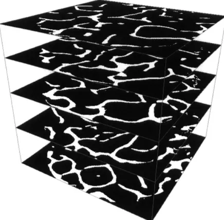
The first step is to get a vertical stack of 2D images, or zstack, as shown in 3-9. Each image is a pixel in thickness and several hundred pixels in width and length. For this study, slices of pCT images were obtained from Prof. Niebur from Notre Dame University.

The stack of images can be processed using various techniques in order to create a three-dimensional finite element mesh. This allows us to get a solid representation of bone that is anatomically correct.

To mesh the images, the Marching Cubes algorithm for 3D surface reconstruction was used. It was developed by Lorensen and Cline [22] and included as the algorithm in the Amira meshing software. This method was used because it results in smoother meshes. It works by creating a cube between two slices of images such that the cube vertices are at the midpoints of the pixels, as shown in Figure 3-7. It then assigns a label, either 1 or 0 to each vertex, based on the color. The cube is composed of 8 vertices, 4 for the top slice and 4 for the bottom slice.

Depending on the labels of the marching cube, a triangulation is chosen to represent that box of volume in the mesh. Figure 3-8 shows some triangulation choices for

Length: 0.196 mm

Radius: 0.0684 mm

Angle: 54.740

Slice k + 1 _Z ,1,k+1) 1,.i+ 1 1) 0, , k+11) i+1,', 1 0 (i,j+ ,k) (l+1,j+ Slice k (,Jk(+,k pixel

Figure 3-7: Marching cube used for mesh triangulation placed between two slices of images, as shown by Lorensen and Cline [22].

certain combinations of labels. Therefore, this method takes into account the sur-rounding labels in order to create triangulations at angles that best represent the true shape of the solid.

3.2.1

Meshing Procedure

The meshing process is outlined in detail below. It begins with the p-CT images which, as shown in Figure 3-9 capture the anatomical details in every slice. Here, we can see 5 of the 371 layers of images that make up the vertical representation. The first part of the preparation and meshing process was done using Amira and the second part was done using Ansys.

Steps in the meshing process:

1. Import pCT images into ImageJ and convert to binary.

2. Import resulting piCT images into Amira.

3. Within Amira create a z-stack of images, which together represent the full 3D

volume. Here, the orthoslice and bounding box can be viewed to check that the physical volume is represented by the images as desired.

O~1~2

1301

Figure 3-8: Triangulated cubes based on label combinations taken from each vertex of the cube, as shown by Lorensen and Cline [22].

4. Label each voxel by selecting an RGB color threshold to distinguish empty space from solid space.

5. Generate a surface and apply smoothing to create a 2D surface mesh.

6. Prepare and correct the surface mesh using original geometry information. The

prepare tetragen options allows you to correct issues related to aspect ratio, dihedral angle, intersecting elements, and coplanar triangles.

7. Export the geometry as vrml.

8. Import the geometry into Ansys.

9. Fill the surface mesh to create a 3D volume mesh using tetrahedral elements. 10. Improve the 3D mesh by removing disconnected mesh sections and hanging

Figure 3-9: Layered stacks of segmented binary images of trabecular bone taken from

pCT and imported in AMIRA. Each slice consists of 384x384x1 pixels. There are 371

slices in the z direction.

11. Convert Ansys mesh into Summit format for use with the Summit code.

Figure 3-10 shows the surface reconstruction of the geometry created from trabec-ular bone pCT images as well as the final mesh that results from processing those images.

There are two mesh samples used throughout the study. The samples come from the femoral neck of a 53 year old male. Sample A is the mesh sample shown in Figure 3-11(a) and measures 2 mm in width and 2.5 mm in length. Sample B is shown in Figure 3-11(b) and measures 8 mm in diameter and 10 mm in length.

The process outlined in Section 3.2.1 allows us to achieve smooth, high quality meshes such as the one shown in Figure 3-12(b). If instead the mesh is automatically filled,

the resulting mesh will contain imperfections and cavities such as the one shown in Figure 3-12(a). Working on every aspect of mesh generation, beginning with the image and ending with the full three-dimensional mesh, eventually results in a high quality mesh that can capture the details of the trabecular architecture. According to an Ansys evaluation, 23.981% of the elements have near perfect aspect ratios falling between 0.891 and 0.9405, with an aspect ratio of 1.0 representing an equilateral geometry. Additionally, this higher quality mesh can progress further in applications without reaching stability issues.

(a) Side view of trabecular bone sur-face reconstruction from pCT images in Amira

(c) Top view of trabecular bone surface recon-struction from pCT images in Amira

b) Side view of trabecular bone mesh in Ansys

(d) Top view of trabecular bone mesh in Ansys

Figure 3-10: Trabecular bone mesh after processing pCT images in Amira and then meshing in Ansys to create a mesh consisting of 2, 379, 141 linear tetrahedral elements.

(a) Sample A consisting of 67, 114 tetrahedral ele-ments generated from a subset of pCT images which measure 1/4 of the total image dimension in direc-tions x and y.

#Z

(b) Sample B consisting of 2,379,141 tetrahedral

elements generated from the full pCT images.

(a) Three-dimensional trabecular bone mesh gener-ated directly from images without AMIRA process-ing. There are visible gaps and cavities along the surface.

(b) Three-dimensional trabecular mesh generated by

segmenting the binary images, creating a surface mesh with AMIRA, and filling the volume in Ansys.

Figure 3-12: Zoomed in image of part of the trabecular bone mesh in the same vicinity for meshes created using different processes. The mesh that results from AMIRA and Ansys is a higher quality mesh.

Chapter 4

Material Behavior Modeling of

Trabecular Bone

4.1

Previous Models in Literature

Several material models have been reported in the literature that try to capture the constitutive behavior of bone. Small deformation in bone has been studied using the St.Venant-Kirchhoff model. Although this is a hyper-elastic model, it extends to the nonlinear range and has been used to study the material behavior of bone for deformations of up to 0.5% strain

[45].

Other models have been developed by using finite deformation kinematic equations. These models consist of a purely elastic linear material model combined with a plastic-ity model. Yield surface information from trabecular bone has been used to implement plasticity models such as Drucker-Prager and Mohr-Coulonb [20]. Another version of a plasticity model [49] used a negative post-yield modulus to capture the softening behavior. More advanced models have also incorporated rate sensitivity

[4]

4.2

Constitutive Equations

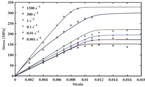
Recent work by Johnson, et al. ?? characterizes cortical and trabecular response at different strain rates by using a visco-elastic, visco-plastic constitutive model. They also plot their simulation results alongside experimental values to show the correlation

[15]. 350 * 1500 S 300 _{o s300s} 250 - * 1 o 0.1s 200 0 0.01 s~ 0 o 0.001s * n * 150 o o 0 100 50 0 0.002 0.004 0.006 0.008 0.01 0.012 0.014 0.016 0.018 Strain

Figure 4-1: Stress-strain solid curve fits from the Johnson constitutive pared with data points from the McElhaney experiment. [15]

model

com-The model has been calibrated and shown to capture the correct behavior of cortical and trabecular bone [15]. The schematic shown in Figure 4-2 represents the model used to capture the material behavior of bone and illustrates the elastic, visco-elastic, and visco-plastic sections.

To capture the visco-elastic behavior of bone, two visco-elastic regimes are required. The first, q1, represents viscosity in the low strain rate regime. The second, q2, has a

shorter time constant and is intended to capture the stiffening behavior that arises in high strain rate cases. The model used by Johnson is Maxwell-Weichert and can be described by Equation 4.1, where VE represents the visco-elastic component of the

total strain:

Est -Egt

o-(t) = EoiVEt + TI VE(1 - e

)

Subscript 0 represents the elastic or long-term equilibrium mechanism and subscripts

1 and 2 represent the first and second visco-elastic mechanisms, respectively. Due to

the observed dependence of yield stress on strain rate, a visco-plastic component mod-eled by the Ramberg-Osgood equation was also incorporated by Johnson in Equation 4.2:

j.P

T

0( o)

(4.2)

lo-

The VP exponent represents the visco-plastic mechanism. So is the Ramberg-Osgood plasticity stress and m is the Ramberg-Osgood exponent. To completely describe the material model, the strain contributions from each of the mechanisms are added in Equation 4.3 to fully represent the model:

5= +V VP (4.3)

E, Ez

Eo E Viscoelastic

111 112

So, m Viscoplastic

Figure 4-2: Constitutive model schematic representing visco-elastic, visco-plastic bone

Material Properties

Eo [GPa] E1 [GPa] E2 [GPa] 71 [MPa s] 772 [kPa s] So [MPa] m p [kg/m 3

16.2 4.4 23.5 132 227 222 18.24 1810

Table 4.1: Material properties specified by the user to describe trabecular bone, calibrated with McElhaney experiments [15].

4.3

Implementation in Summit

The User-defined MATerial model subroutine (UMAT) was previously developed for use in Abaqus. In order to make it functional for the Summit finite element frame-work, a few changes had to be made.

First, a new material was defined within the Materials Class and assigned an identifi-cation value at the top level of the material code. Then, a C interface was developed and used to communicate between the Fortran UMAT and the C and C++ code. Methods were defined to call the Fortan constitutive methods with data from the Summit code used here. Arguments used here were consistent with the arguments of the material subroutine. Lastly, variables were created to store properties read from the user-defined materials file. Properties can be seen in Table 4.1.

Chapter 5

Modeling Framework

5.1

Computational Framework

In order to model dynamic impact problems, the Summit computational solid me-chanics solver was used. This Lagrangian finite element solid solver was developed

by the Radovitzky group as described in

[37]

5.2

Finite Deformation Numerical Formulation

In the continuum framework, the deformation gradient tensor F relates displacements in the current configuration to displacements in the reference configuration via the following relation:

dx.

Fi1 = *(5.1)j

dX1

repre-sents the reference configuration. The deformation mapping <p (X, t) is also a measure of the current displacement as shown in equation 5.2.

Fi1 _ dxi (5.2)

OXI dXj

The Jacobian J of the deformation is defined as the determinant of the deformation gradient tensor J = det(F). It represents the ratio of the change in volume in the current configuration to the change in volume in the reference configuration. The First Piola-Kirchhoff stress tensor relates stresses in the current configuration to areas in the reference configuration, as shown in equation 5.3. o is the Cauchy stress.

Pa =Jo-isF7j T _(5.3)

The problem is governed by the continuum equation for linear momentum balance. The strong form is presented in equation 5.4. Here Vo is a material gradient, po is initial density, and N is the unit surface normal in the reference configuration.

po' = V o.pT +poB in Bo (5.4)

Displacements are specified on Dirichlet boundary conditions: p = < on &DBo

Tractions are specified on Neumann boundary conditions: P - N = on ONBO

Next, the weak form is presented in equation 5.5, integrated in every element and summed over all elements. Here ch is an elementwise-continuous polynomial

approx-imation of the deformation mapping. 6