Data-driven path filtering in ConceptNet

Data-Driven Path Filtering in ConceptNet

by

Yilun Zhou

B.S.E., Duke University (2016)

Submitted to the Department of Electrical Engineering and Computer

Science

in partial fulfillment of the requirements for the degree of

Master of Science in Electrical Engineering and Computer Science

at the

MASSACHUSETTS INSTITUTE OF TECHNOLOGY

June 2019

Massachusetts Institute of Technology 2019. All rights reserved.

Signature redacted

A uthor ...

Department of Electrical Engineering and Computer Science

May 23, 2019

Signature redacted

C ertified by ...

Julie A. Shah

Associate Professor of Aeronautics and Astronautics

Thesis Supervisor

Signature redacted

SIvNte vTE... ....

MASSACHUSErTs INSTMUTE

-j-OF TECHNOLOGY

.ese

A.

Kolodziejski

Professor of Electrical Engineering and Computer Science

JUN

13

2019

_{Chair, Department Committee on Graduate Students}

Data-Driven Path Filtering in ConceptNet

by

Yilun Zhou

Submitted to the Department of Electrical Engineering and Computer Science

on May

23, 2019, in partial fulfillment of the

requirements for the degree of

Master of Science in Electrical Engineering and Computer Science

Abstract

In many applications, it is important to characterize the way in which two concepts are

semantically related. Knowledge graphs such as ConceptNet provide a rich source of

in-formation for such characterizations by encoding relations between concepts as edges in a

graph. When two concepts are not directly connected by an edge, their relationship can still

be described in terms of the paths that connect them. Unfortunately, many of these paths are

uninformative and noisy, meaning that the success of applications that use such path

fea-tures crucially relies on their ability to select high-quality paths. In existing applications,

this path selection process is based on relatively simple heuristics. In this thesis I instead

propose to learn to predict path quality from crowdsourced human assessments. Since a

generic task-independent notion of quality is concerned, human participants are asked to

rank paths according to their subjective assessment of the paths' naturalness, without

be-ing given specific definitions or guidelines. Experiments show that a neural network model

trained on these assessments is able to predict human judgments on unseen paths with near

optimal performance. Most notably, the resulting path selection method is substantially

better than the current heuristic approaches at identifying meaningful paths in various

ap-plications.

Thesis Supervisor: Julie A. Shah

Acknowledgments

First of all, I would like to thank my advisor Professor Julie Shah for guiding me through this thesis research. Although I was started in an existing project, she made sure that I had enough freedom to choose a direction that I was genuinely interested. At the same time, she also kept me on the correct direction, despite my frequently occurring random thoughts trying to make me stray away.

In addition, I am indebted to Professor Steven Schockaert, who is an external collab-orator working with Julie and me on this project. He is immensely knowledgeable in this area, and always able to provide insightful suggestions. After Julie got him involved in the project, he was involved in all the technical details, from modeling to experiment anal-ysis. Throughout the process, I learned a lot about how to design models, how to come up with targeted experiments, and finally how to clearly communicate the results both in writing and orally. Especially during the revision process, without his critical evaluations, this thesis would never be nearly as mature and comprehensive as it currently is.

In addition, the Interactive Robotics Group has been a valuable resource to go to for whatever I need. Other than having research-related discussions, I also enjoy the weekly lab lunch and informal social gatherings with the lab members. I would like to specifically thank Serena Booth, Joseph Kim, Shen Li and Mycal Tucker for having me in helpful discussions and out-of-work social activities.

Finally, I would like to thank my parents, without whose support I would never be here. Through their hard work, I was able to get all the necessary preparations to pursue my passion in my life during college and graduate school, which really is a luxury that I would not trade for any amount of money.

Contents

1 Introduction 13 2 Related Work 17 3 Method 21 3.1 Problem Formulation . . .. . . . . 21 3.2 M odel . . . . 22 3.3 Training . . . . 24 3.4 Features . . . . 26 3.4.1 Vertex embedding (300) . . . . 26 3.4.2 Vertex frequency (1) . . . 26 3.4.3 Vertexdegree(1) .. . . . 26

3.4.4 Vertex sense score (1) . . . 26

3.4.5 Edge ends similarity (1) . . . . 27

3.4.6 Edge direction (3) . . . . 27

3.4.7 Edge relation (46) . . . . 27

3.4.8 Edge provenance (6) . . . . 27

3.4.9 Edge sense score (1) . . . . 28

3.4.10 Sense score calculation. . . . . 28

4 Experiments 31 4.1 Data Collection ... .. .. .. .. ... . . .. .. . . .. . . . .. . .. 31

4.3 Prediction Accuracy . . . . 4.3.1 Experimental Setup . . . . 4.3.2 Quantitative Analysis . . . . 4.3.3 Qualitative Analysis . . . . 4.4 Ablation Study on Feature Importance . . .

4.5 Naturalness as a Path Selection Criterion . . 4.5.1 Semantic Coherence . . . . 4.5.2 Information Retrieval . . . . 4.5.3 Analogy Inference . . . . . . . . 33 . . . . 33 . . . . 36 . . . . 37 . . . . 39 . . . . 40 . . . . 40 . . . . 41 . . . . 44

List of Figures

3-1 LSTM model architecture. Blue (bottom) cells represent raw features (of variable lengths). Green (middle) cells represent transformed features (of length If). Orange (top) cells represent the final code for the vertex (of length if). The encoding of an edge is computed in a similar fashion. The codes (yellow) for vertices and edges are successively processed by an LSTM network. The last state h2,-l (orange) is used as the code for

the entire path. The path codes (orange) first pass separately through fully-connected layers (with shared weight) with an output dimension of 1. A softmax layer then calculates the probability that path

1

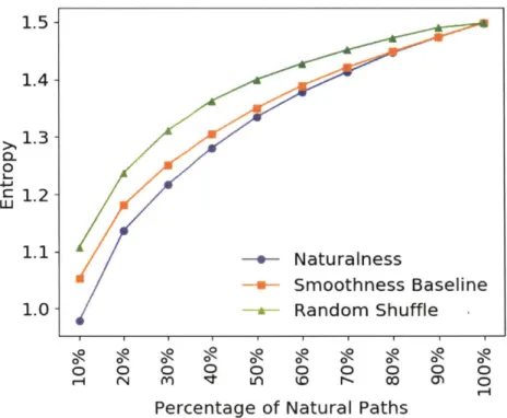
is more natural than path 2. . . . . 23

4-1 Average entropy of path-summarizing relations for different proportions of natural paths. . . . 42 4-2 Performance *of query expansion for hard queries in terms of Precision at

10 (P@ 10, top) and Mean Average Precision (MAP, bottom). . . . 44

4-3 Performance on the 11 analogy questions for which direct connections are not available, using various proportions of natural paths. . . . 46

List of Tables

4.1 Results for the multi-response dataset. . . . . 33

4.2 Pairs of paths with different opinion splits (OS). In each cell the most fa-vored path is shown on top. . . . . 34 4.3 Test accuracy (in percentage) in the domain-specific setting of "science"

related w ords. . . . . 36

4.4 Test accuracy (in percentage) in the transfer learning setting, where the model was trained on the "science" dataset and evaluated on the "money" dataset. . . . . 36

4.5 Test accuracy (in percentage) in the open-domain setting of the most fre-quent English words. . . . . 37

4.6 Best paths of 4 or less nodes between "health" and "computer" ranked by baselines and the proposed model. . . . . 38

4.7 Paths predicted to be among 10% most natural by the learned model, but

10% least natural by the smoothness baseline. . . . . 39

4.8 Paths predicted to be among 10% most natural by the smoothness baseline, but 10% least natural by the learned model. . . . . 39

Chapter

1

Introduction

Many applications require information about the semantic relation between two (or more) words, concepts, or entities. For example, a recommender system needs to recommend items related to a user's browsing history, a task allocation agent needs to match people's experiences and skills to a pool of problems to maximize problem-solving efficiency, and a household robot given the instruction to "wash the plates" needs to infer that a dishwasher could be used. Open-domain knowledge graphs (KGs) such as ConceptNet (Speer et al.,

2017) enable such modeling of semantic relationships in the form of relational paths.

Com-pared to the use of word embeddings (Mikolov et al., 2013) for characterizing relatedness, knowledge graphs have the potential advantage of producing easier-to-understand charac-terizations with explicit relation types, and they can capture relationships that go beyond what is encoded in standard word embeddings (Xu et al., 2014).

Typical knowledge graphs, such as DBpedia and WikiData, are concerned with named entities and their relations (e.g. "Abraham Lincoln" is one of "United States Presidents"). However, this thesis focuses on capturing semantic relationships between common nouns or concepts, which requires a commonsense KG such as ConceptNet. Despite its indis-putable value, however, effectively using ConceptNet in applications comes with a unique set of challenges. The knowledge captured in ConceptNet is, by design, often informal, subjective and vague. Due to the fact that ConceptNet partly consists of unverified crowd-sourced assertions, it is also noisier than many other KGs. Furthermore, many common-sense assertions are true only under some circumstances and to some extent. For example,

ConceptNet encodes that "popcorn" is required for "watching a movie", which captures the useful commonsense knowledge that eating popcorn is associated with watching a movie, but the statement that popcorn is required is nonetheless false. In addition, ConceptNet only disambiguates concepts to a coarse part-of-speech level (e.g. noun meaning vs verb meaning of the word "watch"). Finally, a lot of concepts are linked by the generic "Re-latedTo" relation, which covers relationships as diverse as collocations ("Tire (aedTo

Spare"), hypernyms ("Tire R Tedio All Seasons Tire"), co-meronyms ("Tire Redo

Ex-haust"), homonyms ("Tire RelatedTo Tier"), and very loosely related terms ("Tire RelatedTo

Clothes").

Because of those challenges, few authors use relational paths from ConceptNet in ap-plications. In particular, while several authors have found the knowledge encoded in Con-ceptNet to be highly valuable, they typically restrict themselves to using relationships that are directly encoded as an edge. For example, Speer et al. (2017) showed that ConceptNet can be used to improve word embeddings by incorporating the intuition that words which are linked by an edge in ConceptNet should be represented by similar vectors. I believe that this common restriction to direct edges is due to the lack of sufficiently accurate methods for filtering nonsensical paths, or conversely, for identifying the most natural paths. This path selection problem is the focus of this thesis.

In existing work (Gardner et al., 2014; Lin et al., 2015), the problem of selecting high-quality ConceptNet paths has been addressed in a heuristic way (see Chapter 4). While some intuitions about high-quality paths can easily be formulated (e.g. shorter paths tend to be more informative than longer paths, or the nodes occurring in natural paths tend to have similar word vector representations), such heuristic methods still fail to filter out many nonsensical paths, and conversely sometimes erroneously filter out highly valuable paths. For example, the best path between "lead" and "poison" found by one of the heuristics

(smoothness baseline, see Chapter 4.3) is "Lead synonyn Take DistinctFrom Give RelatedTo

Poison", which uses the verb meaning of "lead", despite the fact that the noun meaning (i.e. the poisonous chemical element Pb) is more relevant in this case.

Rather than trying to construct increasingly intricate heuristics, this thesis proposes to learn to predict path quality using a neural network model. To this end, crowdsourced

assessments about the naturalness of ConceptNet paths are used. Specifically, to collect training data, human annotators were asked to choose the more natural path among a pair of paths, without any guidance on how to interpret naturalness. This notion of naturalness was chosen because it is intuitively easy to understand for crowdsourcers (as opposed to e.g. terms such as "semantic coherence" or "predictive value"). The term is also deliber-ately vague, as I do not want to steer annotators towards particular types of features. The resulting pairwise judgments are then used to train a neural network to predict a latent naturalness score, which can be used for path ranking or path selection.

The main contribution of this work is to show that people's intuitive understanding of naturalness is sufficiently coherent to be used as training data for a data-driven path selec-tion method. To this end, a neural network model is learned to predict latent naturalness scores that are predictive of human pairwise judgments. Results show that the model can predict such judgments with a performance that is close to the optimum suggested by the inter-annotator agreement (Chapter 4.2). For example, the best path found by the model for the above example is "Lead HasProperty, Toxic RelatedTo Lethal RelatedTo _{Poison". In}

addition, for a number of different evaluation tasks, that the method can select semantically more meaningful paths than the previously proposed heuristics.

In the remaining chapters, the thesis is organized as follows. First, I survey related work in Chapter 2. Special attention is paid on applications that use knowledge graph paths, as well as crowdsourcing attempts for knowledge graph acquisition.

In Chapter 3, I present the proposed method. I start by giving a detailed problem for-mulation including the data representation and learning objective. Then I present the model and show how to learn a model from data, while formally proving that the model is indeed learning what should be learned in accordance with the problem formulation. Finally, I discuss the features that are used by the model.

In Chapter 4, I present several experiments designed to study various aspects of the learning performance. First, I describe the data collection procedure. Then I proceed by introducing an inter-annotator agreement study, which empirically estimates to what extent people agree with each other in giving consistent labels on pairs. This study establishes a model-agnostic performance upper-bound and puts the learned model performance in

context. Next I present learning performance results in three settings. Several paths are also shown qualitatively to reveal how our model is better than the baselines. An ablation study follows, which shows relative importance of features. Finally, I use three additional evaluations to show that paths selected by the model have better semantic properties and can lead to improved performance in downstream applications.

Chapter 2

Related Work

Knowledge graphs: KGs explicitly encode relationships between different entities as

subject-predicate-object triples. Such triples can be seen as defining a graph, where the subject and object entities refer to nodes of the graph and the predicates correspond to edge labels. KGs are typically constructed by a domain expert, via crowdsourcing, or

by extracting assertions from a natural language corpus Carlson et al. (2010). This work

uses ConceptNet (Liu and Singh, 2004), one of the most comprehensive commonsense knowledge graphs with 46 relation types, nearly

1

million concepts (words and phrases), and nearly 3 million edges (i.e. triples). It is partly obtained through crowdsourcing, but also incorporates external sources such as OpenCyc (Lenat, 1995), WordNet (Miller et al.,

1990), Verbosity (Von Ahn et al., 2006), DBPedia (Auer et al., 2007), and Wiktionary. Knowledge base construction by crowdsourcing: While the use of crowdsourcing for

constructing knowledge bases has already been well studied, most existing approaches focus on knowledge acquisition. This can involve, for instance, direct collaborative editing of a knowledge base (Bollacker et al., 2008; Vrandei6 and Kr6tzsch, 2014) or indirect construction of a knowledge base through the use of an interactive game (Von Ahn et al.,

2006). In contrast to these works, the focus of this thesis is on using crowdsourcing to learn

path quality perceptions within an existing knowledge graph.

An important challenge with crowdsourcing is the fact that there will inevitably be dis-agreements within the collected data. One framework (Aroyo and Welty, 2014) suggests

that this can be due to (i) the inclusion of low-quality participants, (ii) an ambiguous inter-pretation of the input data and (iii) an ambiguous definition of the labels that crowdsourcers are required to provide. In this work, the first issue is mitigated with a quality control mech-anism (Chapter 4.1). To address the remaining two issues, a probabilistic generative model is proposed to interpret the provided ratings.

Word embeddings: Word embedding methods (Mikolov et al., 2013; Pennington et al., 2014) represent each word in a relatively low-dimensional space of typically 300 dimen-sions, which is estimated from word co-occurrence statistics. With most training proce-dures, vector differences represent abstract relations in the resulting embedding space: for example, Vking - Vqueen Vrnan - Vwoman, in which Vword represents the embedding of a given word.

Both KGs and word embeddings capture aspects of meaning, and can thus to some ex-tent be seen as alternatives. One advantage of word embeddings is that they capture types of knowledge which are difficult to encode symbolically. For example, the cosine similar-ity between word vectors tends to correlate very strongly with human perceptions of word similarity. On the other hand, although related words are often close to each other in the embedding space, it is difficult to "reverse-engineer" and describe the specific relation from the vector difference (Bouraoui et al., 2018). Moreover, when multiple relations exist

be-tween two concepts (e.g. "France Bdrt Germany" and "France

(A11ywith

Germany"),

the vector difference can only reflect an aggregate. Apart from issues which arise because of the use of vectors, there are also some problems that are more generally related to the use of co-occurrence statistics for representing meaning. As a simple illustration of such problems, a system (Krebs et al., 2018) incorrectly assumes that garlic has wings, because of the prevalence of phrases such as "garlic chicken wings".

Given the complementary nature of the KGs and word embeddings, it is perhaps not surprising that several studies have found it to be beneficial to integrate these two types of resources. Some studies (Speer et al., 2017; Faruqui et al., 2015; Xu et al., 2014) reported that knowledge graphs can be used to improve embeddings to achieve better results on vari-ous benchmark tasks such as synonym selection and analogy question solving. Conversely, embeddings can also be incorporated into methods that rely on paths in knowledge graphs,

for example to cluster such paths (Gardner et al., 2014), or as features for a path selection method, as in this work.

Path Features in Applications: Several prior works have described systems that

incorpo-rated knowledge graph paths as features. For example, Boteanu and Chernova (2015) used ConceptNet to solve analogy questions (e.g., "dog is to animal as banana is to fruit") by comparing similarities between paths. Lin et al. (2015) proposed models for learning the embeddings of paths and showed that they performed better on problems such as relation prediction compared to embeddings computed by previous methods. Guu et al. (2015) pro-posed to answer compositional queries (e.g., "Q: What is the population of the capital of Russia?" "A: Russia Capital Moscow Population 12.2 million") by traversing the knowledge

graph in vector space, representing traversal as a series of matrix-vector multiplications. Das et al. (2017) proposed a recurrent neural network (RNN) model with attention mech-anism to reason over entities and relations in a knowledge graph, and observed improved performance in path query answering upon that by Guu et al. (2015).

Among many applications, knowledge graph completion (i.e., inferring missing rela-tions from existing paths) has been a popular target. Lao and Cohen (2010) used path fea-tures for knowledge graph completion in the path ranking algorithm (PRA). Gardner et al. (2014) incorporated embeddings of the relations, allowing the system to recognize seman-tically similar relations, such as "(river) runs through (city)" and "(river) flows through (city)." Neelakantan et al. (2015) built upon the same PRA idea, but used an RNN to model paths. Toutanova et al. (2016) proposed a dynamic programming algorithm that can incorporate both edge and vertex features and reported better performance on knowl-edge graph completion. While all of the above-mentioned knowlknowl-edge graph completion works use some version of PRA to generate paths, Xiong et al. (2017) trained a reinforce-ment learning agent for path generation that rewards accuracy, efficiency and diversity, and demonstrated better performance than PRA-generated paths.

Path Selection: The number of paths between two nodes in a knowledge graph tends to

grow exponentially with path length. In addition, while each type of path can be viewed as encoding a kind of semantic relationship, for many paths this relationship is difficult to interpret. Thus, all of the works described above mitigate the scalability and/or quality

problem via heuristics. To limit the number of paths, Boteanu and Chernova (2015) stopped the path search after a pre-defined number of nodes are explored. Lao and Cohen (2010) and Guu et al. (2015) limited the maximum path length. To obtain natural paths, Gardner et al. (2014) favored paths that contain words with higher embedding similarity. Lin et al.

(2015) calculated the quality of paths using a heuristic based on vertex degree and network flow.

While ConceptNet has been proven useful, most works only use direct edges, with few works (Boteanu and Chernova, 2015; Kotov and Zhai, 2012) being notable exceptions. For other types of knowledge graphs, it was already shown that incorporating longer relational paths can be highly beneficial, and there is no reason to assume that this situation would be any different for ConceptNet. For instance, while there is an intuitively obvious seman-tic relationship between the words "beach" and "sun", there is no direct edge connecting these words in ConceptNet. However, this relationship can be uncovered by observing that

ConceptNet contains the path "Beach (Reedo> Sunbathing R eatdo Sun". Nevertheless,

to enable more effective use of such relational paths from ConceptNet, I believe that more work is needed on how to avoid nonsensical paths, which is the focus of this thesis.

Chapter 3

Method

3.1

Problem Formulation

The end goal is to train a classifier for predicting path quality based on crowdsourced infor-mation. Specifically, human annotators were asked to assess the naturalness of ConceptNet paths. Rather than trying to provide guidelines on how naturalness should be understood,

I simply rely on annotators' intuitive understanding of this notion. This has several

advan-tages, including the fact that annotators are not steered towards particular indicators and the fact that this makes the annotation task much easier. Moreover, given that I am interested in a task-independent form of path quality (i.e., the focus is on eliminating nonsensical and uninformative paths, rather than on selecting the best paths for a particular application), it is not clear what further guidance would be meaningful for annotators. As will be discussed in more detail in Chapter 4.2, despite the lack of guidance on how naturalness should be understood, a high inter-annotator agreement is observed in practice.

Clearly, however, asking participants to provide ratings on an absolute scale is prob-lematic: people have varying thresholds for naturalness, and these thresholds may also change over time. After observing a large number of unnatural paths, people may lower their thresholds to be more willing to accept a path as natural, and vice versa. Therefore, pairwise comparisons are used: selecting which of two given paths is more natural. In this setting, if one path is more natural than the other, two raters would provide the same answer even if they maintained different absolute naturalness thresholds, or if they shifted

their underlying absolute threshold unconsciously over time.

If the two paths are equally (un)natural, the selected answer would be more or less arbitrary, and even the same annotator might not consistently give the same answer when presented with the same pair more than once. Therefore, I propose to model answers to these pairwise comparison questions as probabilistically generated from a latent naturalness score. Specifically, each path is assumed to have a latent naturalness score m, such that for a pair paths with scores m, and M2, the observed answer is drawn from a Bernoulli

distribution, with probability e"l/(eml + eM2) that the first path is selected. While this model allows the less natural path to be selected with some probability, this probability vanishes exponentially with decrease in the latent score. Thus, the learning problem is to predict the naturalness score m of a given path, using crowdsourced answers of pairwise comparisons as the supervision signal.

3.2

Model

In the big picture, the learning model consists of an encoder and a pairwise predictor. The encoder is a long short-term memory (LSTM) network (Hochreiter and Schmidhuber,

1997) that transforms a path into a code vector. The predictor then takes the path codes

and computes the probability that one path is more natural than the other. Each path is represented by an alternating sequence of vertex and edge representations, (v1, ei,

v

2, e2, ... ,

en_1, Vn). Each vertex is represented by a list of n, features, vi = (vi,, vi,2, ..., Vi,n,), with

j-th feature being a dj-dimensional vector. Similarly, each edge is represented by a list of

ne features, ej = (ei,1, ei,2, ..., ej,ne), with j-th feature being a dj-dimensional vector. The

Vertex Code

ReL C R C

Embedding Degree Frequency Sense

(a) The encoding of a vertex.

Output Output Output

-

-

-I LSTM I v, Code el Code LSTM LSTM v₂ Code Path Code Output LSTM v,, Code

(b) The encoding of the path.

Path 1 Code FC FC M2 Path 2 Code S Pr(path 1 is better) em, Z/ eml+eMz

(c) The predictor model.

Figure 3-1: LSTM model architecture. Blue (bottom) cells represent raw features (of vari-able lengths). Green (middle) cells represent transformed features (of length 1f). Orange (top) cells represent the final code for the vertex (of length 1f). The encoding of an edge is

computed in a similar fashion. The codes (yellow) for vertices and edges are successively processed by an LSTM network. The last state h2n-1 (orange) is used as the code for the

entire path. The path codes (orange) first pass separately through fully-connected layers

(with shared weight) with an output dimension of 1. A softmax layer then calculates the

probability that path 1 is more natural than path 2.

Thus, vertex and edge representations must first pass through an encoder. Figure 3-la depicts how a neural network encodes a vertex into a vertex code of pre-defined length if. Each feature (such as the word embedding and absolute frequency in some large corpus) is transformed through a rectified linear unit (ReLU)-activated fully-connected (FC) layer to a vector of length If. The overall code is the average of the vectors. The encoding of an edge to the same length If is conducted in a similar fashion. Figure 3-lb depicts the way in which the path code is calculated. After the codes for each vertex and edge are computed, they are sequentially aggregated by an LSTM network. The last state h2,- ₁ is

interpreted as the code of the path. As shown in Figure 3-

1c,

the predictor then outputs the pairwise comparison result. It first transforms each path code to a score (Mi and m2) using

linear layers with shared weight. The softmax function is then applied to the two scores to calculate a probability. While the network predicts pairwise comparisons, it is the score mi produced by the network - or, at least, the ordering induced by the scores - that matters for applications.

The problem falls under the broad umbrella of learning to rank, for which many algo-rithms have already been proposed. an LSTM encoder is used because for its flexibility with variable length input, while most other methods can only take fixed length input rep-resentations.

3.3

Training

The negative-log-likelihood (NLL) loss is used as the objective function, along with the Adam optimization algorithm (Kingma and Ba, 2015). Although the neural network model seems like a natural choice for the data generation process described in Section 3.1, here

I show that the predicted scores m indeed converge to the latent scores from which the

pairwise comparison results were generated, up to a constant difference.

Consider two paths with scores min and M2. According to the generative model, the first path is selected with probability pmm2 - e"1 /(eM + eM2). Note that from em' /(e" +

eM2) -em

/

(em

+

e") it follows that m -m = ₂ - m' by simple algebra. This means

it must be the case that there is a fixed constant c such that for each path with naturalness score m, the predicted naturalness score m' is such that m = m' + c.

It remains to be shown that the NLL objective will indeed lead the neural network model to predict the correct probabilities. Specifically, assume that observations {yi - Bernoulli

(qO(X))}In=1 are given, where xi is the feature representation of a given pair of paths and qo(xi) is the corresponding output of the neural network model when the parameters are set as 0. To show that minimizing the NLL objective will result in parameters

4,

such that

qg = qO, note that for any fixed xi, given a set of observations {(xi, Yi ... , (xi, yini)}, the

expected data likelihood with respect to qi is defined to be:

Eqi [P r (yi, 1:.,1 xi) = E

[

[yi, qi + (1 - yiy)(I - qi) .j=1

When Yi,1 :n is generated by Bernoulli (qo(xi)), it can be shown that arg maxq Eqi [Pr(yi,i:ni x) = qO(xi). For the entire dataset {(x1, yi), .., (xn, yn)}, since the yi's are independent of

each other given xi, the expected joint likelihood for the entire dataset

Eq, [Pr(y:nlx:n)] E [yjqO(xj) + (1 - yj)(1 - q4(xj))]

j=1I

is then maximized for q(x) qo(x) for all x. Therefore, minimization of NLL (i.e. - log [Pr(y1inx1:n)]) achieves the objective.

Emphatically, the network will converge to optimal predictions even with only one answer for each pair, which can be used to maximize the diversity of the crowdsourced annotations: by only collecting a single annotation for each pair of paths, a broader range of paths can be assessed (with a fixed budget) than with multiple annotations per pair. While each individual answer will to some extent be arbitrary (e.g., the fact that path

1

was selected could mean that path

1

is more natural or that both paths are approximately equally natural and that path

1

was selected by chance), because the network is trained on many different pairs, it will still learn to differentiate between clear-cut cases and borderline cases.

3.4

Features

The features used to encode vertices and edges are described below. The number in paren-thesis after each feature name indicates the dimension of that feature.

3.4.1

Vertex embedding (300)

This feature is taken directly from the 300-dimensional GloVe (Pennington et al., 2014) embedding, pre-trained on the Common Crawl' dataset with 840 billion words. In some experiments, principal component analysis (PCA) is used to first reduce the dimensionality of this feature before inputting it into the neural network.

3.4.2

Vertex frequency (1)

This feature is a scalar representing the frequency of the given word, which can be esti-mated using Zipf's law (Zipf, 1935) from word occurrence ranks. The word occurrence rank is also computed by and available in GloVe embedding data. For example, the word

"science" is ranked 717th, and is thus assigned a frequency of

1/717=1.39e-3.

3.4.3

Vertex degree (1)

This feature is the number of neighbors (in both directions) of the vertex in the graph, representing how well connected the word is within ConceptNet.

3.4.4

Vertex sense score (1)

This feature is a number between 0 and

1

representing how consistent is the overall meaning of the vertex compared to its neighbors on the left and right. For example, the sense score for the word "book" in the path "Knowledge

THaA

Book

(ReaedTo

Restaurant" would be quite low because it is used in two different senses . On the other hand, the sense score for

"book" in "Knowledge

(HasA

Book RelatedTo Paper" would be high. A lower sense score is

hypothesized to result in the path being considered less natural. In calculating this feature, lhttp://commoncrawl.org/

I borrow and extend the idea of "word sense profile" proposed by (Chen and Liu, 2011). The details are left to the end of this section.

3.4.5

Edge ends similarity (1)

For an edge connecting two vertices (s, t), this feature is the cosine similarity of the em-beddings of s and t.

3.4.6

Edge direction (3)

This feature is a one-hot vector that represents if the edge is forward ("Dog IA Animal"), backward ("Wheel (HasA Car"), or bidirectional ("Big "to"y") Small").

3.4.7

Edge relation (46)

This feature is a one-hot vector that represents the relation type of the edge.

3.4.8

Edge provenance (6)

In ConceptNet, each edge is derived from at least one source. In the case of multiple sources, the weight is the sum of the weights across all sources. However, weights across sources are not directly comparable; for example, nearly all edges from WordNet have a weight of 2.0, while those from Wiktionary have a weight of 1.0. This does not neces-sarily mean that WordNet is more reliable than Wiktionary. Thus, the provenance of an edge is represented using a 6-dimensional vector, with one component for each possible source: WordNet, DBpedia, Verbosity, Wiktionary, OpenCyc, and Open Mind Common Sense (Singh et al., 2002). When an edge has only one source, its component in the vector has a value equal to the weight, and all other entries are 0. When an edge has multiple associated sources, the weight is split across the sources using the most common weight of each source (e.g., 2.0 for WordNet).

3.4.9

Edge sense score (1)

Similar to the vertex sense score, this feature is also a number between 0 and

1

character-izing the consistency of meaning, but at an edge level. The details are found below.

3.4.10

Sense score calculation

Since ConceptNet does not distinguish between senses of a given word, this feature cap-tures the intuition that paths mixing different senses of the same word will be perceived as less natural; for example, "Knowledge (HasA Book (RelatedTo0 Restaurant" may be nonin-tuitive since the word "book" is used in two different senses: "something to read" in the first part, and "reserve (accommodations, a place, etc.)" in the second. Moreover, not all senses are "equidistant" from each other; for example, the second part of the path

"Knowl-edge (HsA Book

!IA

Notebook" incorporates yet another sense of "book": "a collection

of blank pages to write on." However, the change in meaning is much less significant in this path, and as a result this path is perceived as more natural.

Chen and Liu (2011) modeled a sense by its word sense profile (WSP). Using WordNet, the WSP of a sense (e.g., first sense of the word "car") is the union of the following sets of words (words in parentheses are for the "car" example):

1. words in the synonym set (auto, machine, motorcar)

2. IsA relation (ambulance, bus, cab, etc.)

3. HasA relation (accelerator, bumper, roof, etc.)

4. definition excluding stop words (a motor vehicle with four wheels usually propelled

by an internal combustion engine)

Chen and Liu (2011) defined the similarity between two words f""(wi, w2) as the

Nor-malized Google Distance (Cilibrasi and Vitanyi, 2007). However, because Google now rate-limits their query interface, cosine similarity of embeddings is used as the similarity function.

The similarity function of a word and a sense is defined as:

f(w, S) Ew'EWSP(s) fWW(w, w') sWSP(s)|

In practice, when taking the average, only 10 words w' C WSP(s) most similar to w accord-ing to few are used.

For a path consisting of words w1, w2, ... , w,, the most plausible sense for each word is

determined. Specifically, for each word wi, the sense swi for wi that maximizes [fS(wi_ 1,

Swi) + fw,(wi+1, swi)]/2 is found. For boundary words, the only neighbor is used. The

assigned sense for wi is denoted as s*. With this disambiguated path, the sense score for each vertex and edge is calculated.

Vertex sense score The sense score for the vertex vi is:

fW8(wi_1, si) + fw8(wi+1, s*)

max,, f.,(wi_1, s') + max,, fw,(wi+1, s')

Note that the maximum sense score of

1

is attained when the sense s* is the sense most closely related to both wi_1 and wai. This is intuitively the case if the edges (wi- 1, wi)

and (wi, wi+i) are based on the same sense of word wi. Also note that the sense score for the first and last vertices is

1

by design.

Edge sense score The sense score for the edge ej = (vi_ 1, vi) is:

fW8(wi_, si*) + fW8(wi, s*_1)

Chapter 4

Experiments

This chapter presents the experimental findings. It first describes the data collection pro-cedure and then presents an evaluation of the collected data and learned model in several

aspects.1

4.1

Data Collection

For the experiments, Amazon Mechanical Turk is used to collect pairwise human rating data. Each questionnaire consisted of 73 pairs, including 60 genuine pairs and 13 quality-control pairs. The quality-quality-control pairs consisted of an obviously good path and an obvi-ously bad path. The good paths were manually constructed and meant to be very natural and straightforward (e.g., Email UsedFor) Communication

(UdFo

Telephone). To gener-ate bad paths, words and relations were sampled independently at random (e.g., "Beautiful

Is Other RelatedT Them MotivateiBy Rug"). Only answers with all 13 quality-control

questions correctly answered were used. The genuine pairs consisted of randomly sampled paths from ConceptNet. Different strategies to sample paths are used, according to the pur-pose of each experiment, and will be introduced in conjunction with the respective results. Overall, around 1,500 valid responses were collected, resulting in around 90,000 pairs of paths to use in different settings of the experiment.

1_{The code and data for the experiments can be found at https: //github. com/YilunZhou/} path-naturalness-prediction

4.2 Inter-Annotator Agreement

The human annotators were provided with a generic question: "which of the two paths is more natural?" Different participants may interpret this question slightly differently, focus-ing on different aspects of naturalness. Thus, one important question is how much humans agree with each other about naturalness. Establishing the inter-annotator agreement level is also useful because it serves as an intrinsic, model-agnostic performance upper bound.

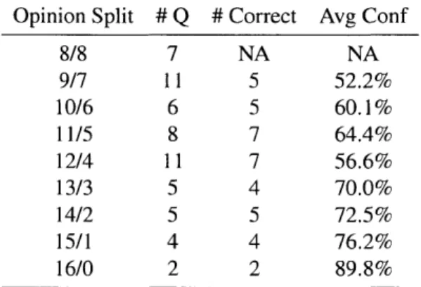
The default data collection strategy is to obtain only one answer for each pair of paths. This strategy maximizes the coverage of the dataset, while still allowing the model to make probabilistic predictions, as discussed in Chapter 3.3. However, to evaluate the inter-annotator agreement, a multi-response dataset is collected, with 59 questions each answered by 16 different participants.

Table 4.1 summarizes the results of an analysis of this dataset. The first column lists the different possible opinion splits for a given question; for example, 13/3 corresponds to a question for which 13 people preferred one of the paths, and 3 people preferred the other. The second column shows how many of the 59 questions have a given opinion split.

The last two columns of Table 4.1 refer to results obtained by the model trained in the

1st

setting described below in Chapter 4.3. The third column shows the number of questions predicted correctly, i.e. the number of questions for which the prediction of the model coincides with the majority opinion of the human participants. The last column is the model's average confidence in the majority opinion. The 8/8 row does not include prediction statistics because there is no majority opinion for these questions.

A number of conclusions can be drawn from these results. First, given the disagreement

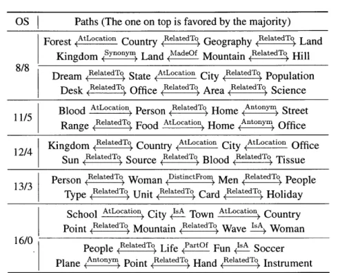
levels shown in the second column, the theoretically best performing model, which always predicts the majority preference, would achieve 70.1% accuracy on this dataset. This shows that while people do not agree with each other on all of the questions, for most pairs, human annotators do have a clear preference. Note that a perfect agreement should not expected, since in some cases both paths may be equally natural or equally unnatural. This is illustrated in Table 4.2, which shows examples of pairs with different opinion splits. As can be seen from these examples, the fact that there is no majority for a given pair does not

necessarily mean that the paths involved are of low quality. It simply means that the two paths are approximately equally natural.

The third column in Table 4.1 shows that, when there is a clear human consensus about which of the two paths is most natural, the trained model can predict this with a very high accuracy; e.g. for all questions where the opinion split was 14/2 or better, the majority view was predicted correctly. Furthermore, there is a strong positive correlation between the con-fidence scores predicted by the learned model, shown in the last column, and the amount of disagreement among human annotators, suggesting that the model can distinguish between cases where the difference in naturalness is clear-cut and cases where human annotators would be undecided.

Opinion Split #

Q

# Correct Avg Conf

8/8 7 NA NA 9/7 11 5 52.2% 10/6 6 5 60.1% 11/5 8 7 64.4% 12/4 11 7 56.6% 13/3 5 4 70.0% 14/2 5 5 72.5% 15/1 4 4 76.2% 16/0 2 2 89.8%

Table 4.1: Results for the multi-response dataset.

4.3

Prediction Accuracy

4.3.1

Experimental Setup

In this set of experiments I studied how well the model can predict human judgements in three settings.

- In the

1st

setting, a set of 100 words is first determined. To this end, starting from the center word "science", a random walk on ConceptNet is performed, considering only elementary-school-level nouns2, until 100 different words had been sampled. Then

2

OS Paths (The one on top is favored by the majority) Forest AtLocation Count Related Geography (RelatedTo Land

Kingdom 4synony"i Land (MadeOf Mountain ( Relatedlo Hill

8/8 Dream RelatedTo _State AtLocation _{City RelatedTo Population}

Desk RelatedTo Office RelatedTo Area RelatedTo Science

Blood AtLocation, Person RelatedTo, Home eAntonyn> Street

__/5 Range . edTo Food At .ation Home ( Y) Office

4 Kingdom (RelatedTo Country (AtLocation AtLocation Office

_/ Sun RelatedTo Source RelatedTo Blood RelatedTo

Pso RelatedTo oa DistinctFronT me RelatedTo

13/3 Person

~eT~Woman

~

en (~di People

13/3 _{TypeRelatedTo Uit (RelatedTo Cr RelatedToHlda}

___ Type 0ed Uni ke~ Card 0e~ Holiday

School AtLocation ACity Town AtLocation Country

Point RelatedTo Mountain (RtedTo Wave

14

Woman

16/0 Pp RelatedTo _{Life Partof Fun IsA Soccer}

Plane

(Antonym

P RelatedTo Hand RelatedTo Instrument

Table 4.2: Pairs of paths with different opinion splits (OS). In each cell the most favored path is shown on top.

the subgraph of these 100 words and all edges in between was used as the knowledge graph. This dataset included about 10,000 paths. The training set contains 40,000 pairs sampled from 8,000 paths (with duplicate paths in sample), and the test set contains 1,000 pairs put together from the remaining 2,000 paths. This evaluation assesses the performance of the system in a domain-specific setting, since the model is evaluated on paths involving the same words as those in the training paths (but nonetheless different paths). This performance is recorded in Table 4.3.

In the 2nd setting, another set of 100 words were collected using the same method as above, but using "money" as the center word, and ensuring that there is no overlap between this set of 100 words and those from the "science" dataset. Then 1,000 paths were sampled in this subgraph, were made into 500 pairs, which I use to evaluate models trained on the "science" dataset. In this way, I can assess the transfer learning performance of the model. This performance is recorded in Table 4.4.

* In the 3rd setting, nouns, verbs and adjectives from the 5,000 most frequent English words in the Corpus of Contemporary American English3 were selected, for a total

of 3,887 words. 80,000 paths of up to 5 nodes were sampled, which were split into 20,000 training pairs and 20,000 testing pairs (ensuring that there are no overlapping paths between training and testing sets). Compared with the 1st setting, this rep-resents much wider coverage of the set of words (i.e., embedding space), but much sparser coverage of paths, assessing the performance of the model in an open-domain setting. This performance is recorded in Table 4.5.

To put the model performance performance into context, the following four heuristic base-lines are considered, all of which have similar mechanics: computing a score for each path (as does the proposed model), and then selecting the path with the higher score.

Source-Target Baseline (ST-B) scores paths using the cosine similarity between the

em-beddings of the source and target words (note that the two paths in a pairwise comparison do not typically start and end with the same words);

Smoothness Baseline (Smooth-B) scores paths using the average cosine similarity of all

word pairs connected with an edge in the path;

Resource Flow Baseline (Flow-B) scores paths using the "path reliability" method

pro-posed by Lin et al. (2015) with the idea that a path is better if there are less branches out of the path;

Length Baseline (Path-B) scores paths solely by their length, and favors shorter paths to

longer ones.

A grid search of two hyper-parameters was conducted: vertex embedding dimension in

{2, 10, 50, 100, 300} and path code length in {1, 2, 5, 10, 20}. For the first hyper-parameter, principal component analysis (PCA) is used for dimensionality reduction. One-hot encod-ings of words is also tried for the 1st setting. For the other settencod-ings, this one-hot encoding cannot be used, because it cannot generalize to unseen words (2nd setting) or scale to a large number of words (3rd setting). In addition, Length-B performance is only available for the 3rd setting, because for the first two settings path length was not explicitly con-trolled for, resulting in the vast majority of paths being of the cutoff length of 4, and path

3

length is not predictive.

Path Code Length

1 2 5 10 20 2 62.1 63.1 65.8 65.3 65.6 . 10 63.6 65.5 65.6 67.5 66.4 9 50 63.7 65.5 66.9 67.4 67.7 E 100 65.4 65.9 66.1 68.2 67.6 300 66.2 66.6 67.6 67.6 67.7 One-Hot 67.0 66.4 67.0 67.5 67.9 ST-B 53.4 Smooth-B 58.0 Flow-B 51.6

Table 4.3: Test accuracy (in percentage) words.

in the domain-specific setting of "science" related

Path Code Length

1 2 5 10 20 2 60.5 64.6 63.9 65.1 65.5 . 10 60.1 61.7 64.8 64.9 64.8 9 50 62.5 62.8 63.1 63.3 64.0 9 100 60.0 61.8 63.1 64.2 64.8 300 58.8 60.5 61.1 62.0 62.1 ST-B 53.9 Smooth-B 55.9 Flow-B 52.5

Table 4.4: Test accuracy (in percentage) in the transfer learning setting, where the model was trained on the "science" dataset and evaluated on the "money" dataset.

4.3.2

Quantitative Analysis

For the first setting (Table 4.3), the performance was relatively insensitive to embedding dimension and code length, as long as both were sufficiently high. However, performance on the 2nd setting (Table 4.4) dropped significantly with higher embedding dimensions,

Path Code Length 1 2 5 10 20 2 61.4 60.5 63.1 62.9 63.3 .A 10 61.2 62.6 65.0 64.9 64.2 . 50 61.6 64.5 64.8 65.4 65.8

s

100 62.0 64.3 65.0 67.9 65.1 300 61.9 63.0 65.7 65.4 65.4 ST-B 52.3 Smooth-B 57.5 Flow-B 46.8 Length-B 55.8

Table 4.5: Test accuracy (in percentage) in the open-domain setting of the most frequent English words.

suggesting an overfitting problem, with an embedding dimension of 2 achieving best gen-eralization performance. This suggests that a model that was trained on one domain can indeed successfully be applied to another domain, as long as the embedding dimension is small enough to allow for sufficient generalization. In the 3rd setting (Table 4.5), a higher embedding dimension is necessary, most likely because the range of meanings is more diverse for this dataset, which includes not only nouns, but also verbs and adjectives.

For all three settings, considering the level of agreement found in Chapter 4.2, the performance of the model approaches the expected performance upper bound. Moreover, the model performs substantially and consistently better than all of the baselines. In fact, in Table 4.5 only one of the baselines is able to outperform the simple path length heuristic

(Length-B), and only in a minimal way.

4.3.3

Qualitative Analysis

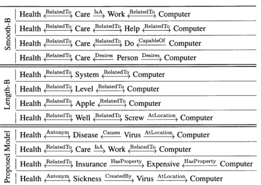
To qualitatively compare how the model prediction differs from the baselines, Table 4.6 presents the best paths between the words "health" and "computer" (of up to 4 nodes)

selected by it and the two strongest baselines.

It can be observed that the top paths found by the smoothness baseline lack variety, most likely due to the high embedding similarity between "health" and "care". In

addi-Health Reaed Care

IA

Work (Raedi Computer HelhRelatedTo ar(RelatedTo Hlp (RelatedTo opue

Health (Idk Care 0) Hel ei Computer 0

E Health RelatedTo Care RelatedTo Do (CapableOf Computer Health RelatedTo Care Desires Person Desires Computer

Health RelatedTo System RelatedTo Computer

Health RelatedTo Level RelatedTo Computer

Health Appleel Computer

RelatedTo RelatedTo

Health RelatedTo Well RelatedTo Screw AtLocation) Computer

Health (Antonyn Disease 4Eaues Virus At Cation Computer

Health RelatedTo Care

A

Work Redio Computer

Related~~o HasProperty aroet

0 Health Reaedoy Insurance H Expensive HasProperty Computer

Health A Sickness C Virus A

Computer

Table 4.6: Best paths of 4 or less nodes between "health" and "computer" ranked by base-lines and the proposed model.

tion, the length baseline does not perform satisfactorily because the shortest paths are not easily understandable without more explanation, with nearly all relations being the generic

RelatedTo". _{By contrast, the proposed model (trained on the 3rd open-domain setting)}

se-lects paths that overcome both drawbacks. It covers a wider variety of concepts such as "virus" and "expensive" and favors longer paths with smoother transition of node seman-tics.

In another evaluation, paths for which the learned model and the smoothness baseline significantly disagree were inspected. To do so, 120,000 paths from the entire ConceptNet graph were sampled and and their quality were predicted using the two methods. Table 4.7 lists paths that are predicted to be among the top 10% most natural by the model but are in the bottom 10% according to the smoothness baseline. Table 4.8 conversely shows paths that are among the 10% least natural according to the model but the 10% most natural according to the baselines. Paths in both tables were selected at random.

As can be seen, the paths in Table 4.7 are intuitively quite meaningful, with all paths using some rather uncommon but relevant words, which is perhaps clearest in the last

ex-Lead HasProperty Toxic (Related Toxicant (yy Poison

Wave

1

Fluctuation RelatedTo Brainwave Derivedrom: Brain Space M Passageway A )ation Building (ad Station Food Tedio? Hechsher RLatedTo Kashrut (RelatedTo Law

Table 4.7: Paths predicted to be among 10% most natural by the learned model, but 10% least natural by the smoothness baseline.

Bee (RelatedTo A RelatedTo After RelatedTo Attack

pae(RelatedTo v RelatedTO RelatedTo oo

Space <~d ery 4e2oLittle edoMoon

ea synony"Rn RelatedTo RelatedTo pig

Lead Soym Run 4e oVery ₄ Le2?.Poison

Adult RelatedTo A Rtedy The RelatedTo English

Table 4.8: Paths predicted to be among 10% most natural by the smoothness baseline, but

10% least natural by the learned model.

ample (Hechsher refers to a certification given to a food product that complies with Jewish religious law and Kashrut refers to the set of Jewish dietary laws). By comparison, the paths in Table 4.8 mostly use very common but uninformative words. This analysis suggests that the smoothness baseline suffers from the so-called hubness problem, i.e. the problem that in high-dimensional vector space embeddings, there are typically a few central objects which are highly similar to many of the other objects (Radovanovi6 et al., 2010), an issue which is known to affect word embeddings (Dinu et al., 2015). The smoothness baseline favors paths with very common words, even if they are not semantically related, because these words act as hubs in the word embedding.

4.4

Ablation Study on Feature Importance

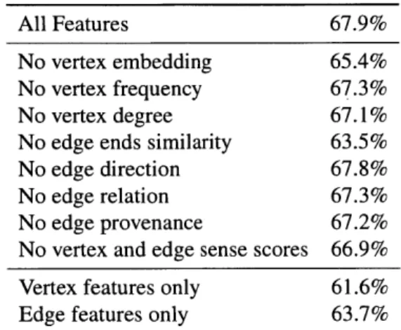
To study the contribution of each feature to the prediction performance, variants of the model with subsets of the full feature set were trained. For this analysis, the 3rd evaluation setting with the best performing hyper-parameters (embedding dimension of 100 and path code length of 10) was used. The results are summarized in Table 4.9.

All Features 67.9%

No vertex embedding 65.4%

No vertex frequency 67.3%

No vertex degree 67.1%

No edge ends similarity 63.5%

No edge direction 67.8%

No edge relation 67.3%

No edge provenance 67.2%

No vertex and edge sense scores 66.9%

Vertex features only 61.6%

Edge features only 63.7%

Table 4.9: Ablation study on feature importance.

most. This is also in accordance with the fact that smoothness baseline in Table 4.5, which only uses this feature, performs best among the four baseline methods. Furthermore, the second-highest reduction is found when leaving out the vertex embedding feature. Finally, neither vertex features nor edge features alone can achieve optimal prediction performance.

4.5

Naturalness as a Path Selection Criterion

Next, three experiments which are aimed at assessing how well naturalness indicates path quality are presented. I start with an intrinsic evaluation of the semantic coherence of natural paths, after which I cover two extrinsic tasks: information retrieval and analogy inference.

4.5.1

Semantic Coherence

First, define the type of a path as the sequence of relations appearing in that path, e.g. the

type of the path "A kI, B HAi c" isA ( 9 HasA ) ). In this experiment, I consider pairs

of nodes in ConceptNet that are connected with a relational path of a given type, as well as a one-step relation (e.g., "A HasA C"). In this situation, the latter relation is called a

path-summarizing (PS) relation for the considered path type. Many path types uniquely

small number. For instance, for a path of type (!I, HasA only ) is expected to be

the PS relation. However, due to the presence of noise in ConceptNet, some relations of this type will actually have a different PS relation. Motivated by this view, as an intrinsic evaluation task, I propose to assess the extent to which a path selection method is able to

select semantically coherent paths in terms of the variability of the PS relations among the

selected paths.

In particular, for a set of paths, I first calculate a mapping from path types to counters of

PS relations: {Pi -+ [(ri, c11), (r₁₂, c₁₂), ..., (rn, cin)], .,Pm -+ [(rmi,cmi), (rm2, cm2),

... , (rmn, Cmn)]}, in which each pi is a path type, each rij is one of 46 relation types from

ConceptNet, and each cij is the number of times the relation rij was found as a PS relation for path type pi. The average entropy of the PS relations is then defined as:

- 1 Ci .E"> Pij ln(pi)] C

where C, =

t

₁ ci3, C = CiPi= ci3

/C

2. A higher average entropy suggest a

higher proportion of spurious PS relations and thus less semantically coherent paths. Using the 3,887 words from the 3rd setting, I generated 126,600 length-4 paths whose source and target nodes are also directly connected by a relation (i.e. the PS relation). The model was applied to rank the paths by naturalness. Based on this ranking, the average entropy of top N% natural paths is calculated, where N varies from 10 to 100, and plot the result in Figure 4-1. The model is compared to Smooth-B, the best-performing baseline for predicting naturalness. The entropy for a random shuffle of the dataset is also depicted for comparison. Using the learned model to select the most natural paths consistently leads to the lowest entropy. Note that all three methods will converge to the same entropy at the

100% mark, at which point all paths are used, regardless of the path selection method.

4.5.2

Information Retrieval

When using a search engine, users often provide under-specified queries, e.g. because they assume that the search engine is "smart" enough to infer their true intention or because they