Quantitative stress imaging by combining static and dynamic elastography

HAL Id: hal-00542868

https://hal.archives-ouvertes.fr/hal-00542868

HAL is a multi-disciplinary open access archive for the deposit and dissemination of sci-entific research documents, whether they are pub-lished or not. The documents may come from teaching and research institutions in France or abroad, or from public or private research centers.

L’archive ouverte pluridisciplinaire HAL, est destinée au dépôt et à la diffusion de documents scientifiques de niveau recherche, publiés ou non, émanant des établissements d’enseignement et de recherche français ou étrangers, des laboratoires publics ou privés.

Quantitative stress imaging by combining static and

dynamic elastography

Heldmuth Latorre Ossa, Jean-Luc Gennisson, Mickael Tanter

To cite this version:

Heldmuth Latorre Ossa, Jean-Luc Gennisson, Mickael Tanter. Quantitative stress imaging by combin-ing static and dynamic elastography. 10ème Congrès Français d’Acoustique, Apr 2010, Lyon, France. �hal-00542868�

10ème Congrès Français d'Acoustique

Lyon, 12-16 Avril 2010

Quantitative stress imaging by combining static and dynamic elastography

Heldmuth Latorre-Ossa1, Jean-Luc Gennisson1, Mickaël Tanter1

1_{Institut Langevin. – Ondes et Acoustique, ESPCI ParirsTech, CNRS UMR7587, INSERM ERL U979, Paris, heldmuth.latorre-ossa@espci.fr}

There is increasing evidence showing the involvement of mechanical-transduction processes in the interplay between shape-related strains and expressions of the genome in living tissues. However, tools allowing long term control of physiological mechanical stress from the inside the tissues lack the investigation of the impact of such processes in organisms. This work presents the feasibility of obtaining a complete bidimensional (2D) map of the stress applied to an elastic soft tissue according to the Hooke’s law (! = E.", where ! is the stress, E is the Young's modulus and and " is the strain). By combining the concepts of dynamic (Supersonic Shear Imaging - SSI) and static elastography, both the elastic modulus (E) and the strain (") can be retrieved respectively. The SSI technique is based on the combination of radiation force induced by an ultrasonic beam and an ultrafast imaging sequence (5000 frames/s) capable of catching in real time the propagation of the resulting shear waves. Then by measuring the shear wave velocity (VS), the complete 2D elasticity map can be retrieved through the

well known expression E = 3#VS², where # represents the density of the media. For the static elastography part,

the tissue is slightly compressed and an ultrasound image is acquired before and after static compression. The cross-correlation between these two ultrasound images allows the determination of the accurate 2D strain map. Experiments were performed on diverse types of agar-gelatin phantoms mimicking soft tissues which present inclusions with different levels of stiffness. The influence of the boundary conditions on measurements is discussed. The mapping of quasi-static stress applied to biological tissues could play a key role in the understanding of tumor mechanical-transduction processes where mechanical stress may induce changes within the tumor structure.

1

Introduction

Palpation is a standard medical practice relying on qualitative estimation of tissue Young’s modulus E =

!

#

where ! is the external compression (stress) and # the tissue deformation due to the applied compression (strain). In order to quantify this practice, two kinds of ultrasound elastography have been developed such as remote sensing technique for imaging the elastic properties of biological tissues in vivo: the so-called static elastography [1] and dynamic elastography [2]. The added value of elastography imaging modalities for medical diagnosis lies in the contrast observed in tissue viscoelastic properties, which correlates with significant changes in the stroma and connective tissues during disease processes. In addition to pathology, the shear elasticity of various normal tissues spans over orders of magnitude [3, 4, 5]. Many studies have shown that strain imaging or quantitative elasticity imaging provide high contrast for many clinical applications such as breast cancer or liver fibrosis staging [6-10]. Specifically regarding static elastography or strain imaging techniques, there is a high amount of literature, which outlines different methods employed to retrieve the value of the strain tensor when dynamic or static compression is applied to a viscoelastic material. However to our knowledge there is no literature available concerning methods to retrieve the value of the stress tensor (stress imaging), owing the fact that those techniques are not able to accurately quantify the value of the tissue Young’s modulus that leads to the stress estimation. The dynamic elastography technique presented in this paper is able to calculate a complete elasticity map of the media under test with great precision, opening the path for the estimation of the stress accurately. This could be of

great importance in mechano-transduction processes of human tissue tumours, in which internal chemical reactions triggered by external mechanical excitation could eventually lead to tumour development. By combining static elastography and dynamic elastography a new parameter can be estimated and be used in order to study such mechano-transduction process. In this paper a classical setup for elastography is presented. Both techniques are used in order to obtain elasticity and strain images of an agar-gelatin phantom which contains two inclusions mimicking soft and hard biological tissues. This procedure allows the estimation of the stress inside media. Cumulative stress is also estimated and the influence of the boundary conditions discussed.

2 Materials and methods

2.1 Measurement Setup

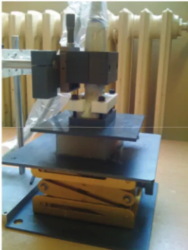
Figure 1 depicts the setup. The phantom lies on a uniform plane surface. The ultrasonic probe was held perpendicular to the phantom’s surface through a support which also held the actuator employed to move the probe downwards. A compressor plate was attached to the probe to guarantee the uniformity of the quasi-static uni-axial compressions. Compression was applied from 0 to 3 mm with steps of 0.1 mm. For each step, dynamic and static elastography were performed.

The dynamic and static elastography parts of the experiments were performed using a conventional ultrasound probe (Supersonic Imagine SL15-4, 256 elements, 8 MHz central frequency) driven by a fully programmable ultrafast imaging device (Supersonic

Imagine Aixplorer). As mentioned before, the measurements were performed on an agar-gelatin phantom (5 % gelatin – 2 % agar) which contains a hard (8 % gelatin – 2 % agar) and soft (3 % gelatin – 2 % agar) cylindrical inclusions with a diameter of 10 mm.

The uni-axial stress was applied through multiple small compressions along the z axis, in order to minimize the negative effects of signal decorrelation caused by large compressions. The idea was to keep the stress as uniform as possible on the top of the phantom to avoid image artifacts originated by the compressor edges. For each compression, dynamic and static elastography measurements were performed as follows.

Figure 1: Measurement setup. The ultrasonic probe and a compressor plate attached to it along with an actuator were

held perpendicular to the phantom by a support.

2.2 Dynamic Elastography - Supersonic Shear Imaging technique (SSI)

The SSI technique is based on the combination of radiation force induced by an ultrasonic beam and an ultrafast imaging sequence (5000 frames/s) capable of catching in real time the propagation of the resulting shear waves. A Supersonic Shear Imaging experiment is divided into two steps: the generation of shear waves and the ultrafast imaging of their propagation. For a detailed description of the basic principle and clinical implementation of this technique, the reader can refer respectively to references [2, 11]. The first step is the generation of a shear wave inside the media by means of the radiation force. Ultrasonic beams of about hundred’s of µs are focused at three different depths in order to generate a plane shear wave. Immediately after the generation of the shear wave, the system switches into an ultrafast imaging mode to acquire a movie of the propagating shear wave. Then by using a time of flight algorithm the shear velocity (VS) is retrieved in each pixels of the image. Therefore it

allows the computation of a complete bidimensional (2D) shear elasticity (µ) map by using Eq. (1), where # represents the density of the media.

2

.

V

µ

%

$

In soft tissues, local stiffness is described by Young’s modulus E and can be approximated by E ~ 3µ. Thus measuring shear velocity leads to Young’s modulus assessment.

2.3 Static Elastography

Elastograms display the strain images that are measured by a static-compression measurement technique where a compressor generates a stress field that deforms a volume of tissue. Local tissue displacements are tracked through changes in ultrasonic echo signals. Strain images are estimated from the gradient of the displacement field [12]. For our experiments, uni-axial quasi-static displacement steps of approximately 0.25% were applied along the z axis (depth) to a phantom whose inclusions have different levels of stiffness. A 2D map representing the axial component of the strain tensor (") was obtained by calculating the first derivative of the displacement along the z axis, where s represents the axial component of the strain tensor and D the displacement along the z axis (Eq. (2)). Due to the fact that the displacement steps and therefore the applied quasi-static compressions are very small, the influence of the lateral component of the strain tensor is ignored and only its axial component is taking into account.

dz

dD

s %

Two radiofrequency (RF) signal sets were acquired: one before and one after compression. Congruent echo lines of each image RF data set were then subdivided into small temporal windows which were compared pair wise using cross-correlation techniques [1], from which the change in arrival time of the echoes before and after compression can be estimated [13]. The resulting values of displacement were then stored in a 2D matrix (displacement matrix) which underwent smoothing and filtering. The 2D mapping of the strain was carried out via Eq. (2) and stored in a 2D strain matrix which was subsequently used for the mapping of the stress. At last from each acquisition step the cumulative

2.4 Stress Map computation

Having retrieved the elastic modulus and strain by means of dynamic and static elastography respectively, the following step was the calculation of a 2D map of the applied stress via the Hooke’s law which states that in linear elastic materials the stress in proportional to the strain (Eq. (3)), where E represents the elastic modulus and " the strain. This procedure was follows for each 0.1 mm compression step.

#

!

%

E

.

The calculation of the 2D Elasticity, Strain and Stress maps was carried out with the software tool Matlab& (Mathworks). The maps which underwent some signal processing through normalization and filtering. The cumulative strain and stress 2D maps were computed by summing up the results at each step.

3

Results

3.1 Elasticity maps

Accurate elasticity maps were obtained through the SSI technique (Fig. 2) where the hard and soft inclusions can be clearly distinguished. The surrounding media for both

inclusions is the same and posses a Young’s modulus value of 8.98 ± 0.47 kPa. The mean values for the hard and soft inclusions Young’s modulus are 24.13 ± 1.50 kPa and 4.34 ± 0.11 kPa respectively.

Figure 2: a) Quantitative elasticity map in kPa (Young’s modulus) of the hard inclusion obtained with the SSI technique. b) Quantitative elasticity map in kPa of the soft

inclusion.

3.2 Displacement and Strain maps

Figure 3 and Figure 4 depict the obtained displacement and strain maps for the hard and soft inclusion respectively.

Figure 3: a) Calculated displacement map in µm around the hard inclusion due to a 0.1 mm compression. b) Dimensionless cumulative strain map computed from the

displacement map. The hard inclusion exhibits smaller strain than its surrounding media.

Figure 4: a) Calculated displacement map in µm around the soft inclusion due to a compression of 0.1 mm. b) Dimensionless cumulative strain map computed from the displacement map. The soft inclusion exhibits higher strain

than its surrounding media.

Displacements are presented for just one of 0.1 mm step. The strains displayed are the cumulative ones from the first to the last acquisition (from 0 to 3 mm). After applying compression, the strain within the hard inclusion is much lower than the one in its surrounding media. The soft inclusion presents an opposite behavior given the fact that most of the strain is concentrated inside the inclusion and only a slight amount is distributed all over its surrounding media.

For each acquisition step, the strain maps were calculated (Fig. 5). The strain values are almost constant and only have a very slight variation for a few compression step over the 30 acquisitions. The slope values of the linear fit for each data lines are smaller than 4.10-4.

Figure 5: Mean strain over four regions of interest: inside the soft and hard inclusion (.), and in the surrounding media

of the soft and hard inclusion (o) for each acquisition step. Figure 6 contains a plot of the cumulative strains of both inclusions and their surrounding media for each compression step. One can note that the strain increases linearly in each case. The surrounding media of both inclusions shows nearly the same behavior.

Figure 6: Cumulative strain inside inclusions and in the media for each compression step of 0.1 mm from 0 to 3

mm.

3.3 Stress maps

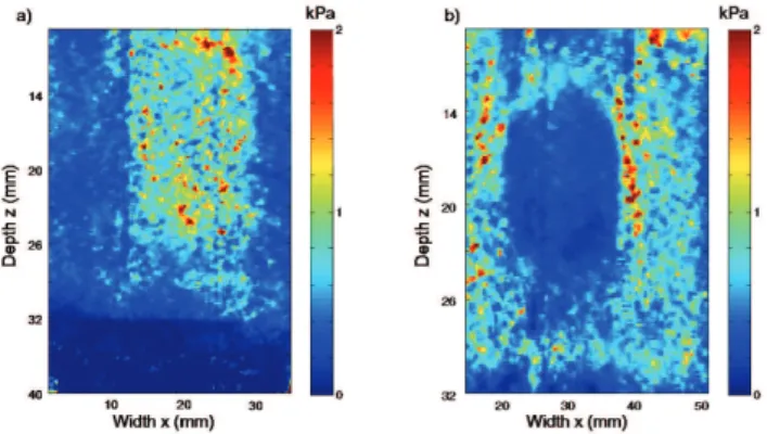
Figures 7 presents cumulative stress maps in kPa for both inclusions over the entire acquisition range. One can notice that the stress is mainly gathered within the hard

inclusion (0.74 ± 0.03 kPa) (Fig. 7a), leaving a slight amount distributed over its surroundings (0.39 ± 0.01 kPa). This is completely opposite to what happens inside the soft inclusion, where the level of stress is smaller (0.25 ± 0.01 kPa) (Fig. 7b) than over its surrounding media (0.67 ± 0.02 kPa).

Figure 7: a) Cumulative stress map for the hard inclusion and b) cumulative stress map for the soft inclusion after the

30th compression step has been applied

4

Discussion

On both inclusions, the displacement decrease rapidly with increasing depth, having their maximum value at the top of the phantom where the quasi-static uni-axial compressions were applied. The computed axial displacements for each inclusion at each compression step were almost equal. Therefore, the strain estimation, which is the first derivative of the displacement along the z axis is almost constant over all the acquisitions (the slope of the linear fit is smaller than 4.10-4). Such a result allows us to affirm that the media was compressed in a linear regime and than the application of the Hooke’s is possible. Nevertheless, the general Hooke’s law is defined for a given volume and the strain is defined as the sum of the strains tensors over the three axes of the Cartesian mark. In our case the strain is reduced to the only axial component # along the z axis (depth axis). This assumption was thus compensated by the use of a compressor plate in order to apply a quasi uni-axial stress to the phantom. Moreover, given that the experiment was performed in a linear regime, we can assume that the axial (z) component of the strain tensor is much higher than the two others, reducing and the calculation of the stress to only one component.

Regarding the inclusions, the soft inclusion shows a much higher strain (approximately 2.3 %) than the hard one (approximately 1.2 %). In terms of elasticity, the Young’s modulus is 6 times bigger in the hard inclusion than in the soft inclusion. This difference points out the quantitative importance of the SSI technique which allows to estimate the true elasticity of a media. Nevertheless, both techniques are in good accordance, a strong elasticity induces small strain and a low elasticity generates strong strain. However, there is a factor of 3 between the values obtained with static and dynamic elastography. This difference can be explained by the fact that the static elastography is strongly influence by the boundary conditions of the inclusions

However stress map were calculated from the multiplication of results, elasticity map and cumulative strain over all acquisitions. To calculate the cumulative

strain, it was necessary to discard the data acquired for the very first compression steps to esure the compressor was completely in contact with the phantom’s surface. This is usually known as pre-compression. For the hard inclusion, the stress is higher than within its surrounding media, something completely opposite to what occurs with the soft inclusion. One can notice that the stress between the top of the inclusions and the phantom’s surface is strongly affected by the inclusion itself. In the case of the hard inclusion, the media between the top of the phantom and the inclusion undergoes two stresses: one from inside the inclusion and one from the top of the phantom where the compressor was placed. It could explain why the stress increases considerably within that region. The opposite can be also notice for the soft inclusion. One can also notice that the values obtained for the stress are in good accordance with the literature, in acoustoelasticity experiments where the knowledge of stress allows to retrieve the shear nonlinearity of a media [14].

5 Conclusion

Through this work, the concepts of dynamic elastography and static elastography were combined to retrieve the value of the applied stress by using the well known Hooke’s law. Dynamic elastography was performed by using the SSI technique whereas static elastography was carried out by applying 0.1 mm uniaxial quasi-static compression displacements on an agar-gelatin phantom. Thus complete 2D elasticity and strain maps of the phantom were retrieved. With all this in hand and by using the Hooke’s law it was possible to calculate an accurate 2D map of the stress. Future work will include the comparison of the results obtained on gelatin-agar phantoms with in vivo and in vitro measurements in order to study the mechanical-transduction processes. Additionally, the acquired data will be compared with finite element simulations. Moreover estimating the stress locally could be very important for nonlinear shear assessment in case of acoustoelasticity experiment, which are easy to implement in vivo.

Aknowledgment

The authors would like to thanks Rémi Souchon for interesting discussion

References

[1] Ophir J., Cespedes I., Ponnekanti H. Yazdi Y., Li X., “Elastography: a quantitative method for imaging the elasticity of biological tissues”, Ultrasonic Imaging, 13, 111-134 (1991).

[2] Bercoff J., Tanter M., Fink M., “Supersonic Shear Imaging: A new technique for soft tissue elasticity mapping”, IEEE Trans. Ultra., Ferro. Freq. Ctrl., 51(4), 396-409 (2004).

[3] Sarvazayan A.P., Redenko O.V, Swason S.D, Fowlkers J.B, Emelianov S.Y., “Shear wave elasticity imaging : A new technology of medical diagnosis”, Ultrasound in Medicine and Biology, 24, 1419-1435 (1998).

[4] Krouskop T.A, Wheeler T.M, Kallel F, Garra B.S, Hall T., “Elastic moduli of breast and prostate tissues under compression”, Ultrasound Imaging, 20, 260-274 (1998).

[5] Kallel F., Ophir J., Magee K., Krouskop T., “Elastographic imaging of low-contrast elastic modulus distributions in tissue”, Ultrasound in Medicine and Biology., 24, 409-425 (1998).

[6] Frey H., “Realtime elastography: A new ultrasound procedure for the reconstruction of tissue elasticity”, Radiology, 43 (10), 850-855 (2003).

[7] Garra B. S., Cespedes I., Ophir J., Pratt S., Zuubier R., Magnat C. M., Pennanen M. F., “Elastography of breast lesions: initial clinical results, Breast Imaging”, Radiology, 202, 79-86 (2002).

[8] Hiltawsky K. M., Kruger M., Starke C., Heuser L., Ermert H., Jensen A., “Free hand ultrasound elastography of breast lesions: clinical results”, Ultrasound in Medicine and Biology, 27, 1461-1469 (2001).

[9] Hall T. J., Zhu Y., Spalding C.S., “In vivo real-time freehand palpation imaging”, Ultrasound in Medicine and Biology., 29, 427-735 (2003).

[10] Barr R. G., Clinical applications of a real time elastography technique in breast imaging. Proc. 5th Int. Conf. on Ultrasonic Measurement and Imaging of Tissue Elasticity 112 (2006).

[11] M. Tanter, J. Bercoff., A. Athanasiou, T. Deffieux, J.-L. Gennisson, G. Montaldo, M. Muller, A. Tardivon, M. Fink, “Quantitative assessment of breast lesion elasticity: Initial clinical results using Supersonic Shear Imaging”, Ultrasound in Medicicine and Biology, in Press (2008)

[12] Bilgen M., Insana M.F., “Error analysis in acoustic elastography. II. Strain estimation and SNR analysis”, Acoustical Society of America, (1997). [13] Ophir J., Cespedes I., Garra B., Ponnekanti H.,

Huang. Y., Maklad N., “Elastography: ultrasonic imaging of tissue strain and elastic modulus in vivo”, European Journal of Ultrasound, 3, 49-70 (1996). [14] Gennisson J.L., Rénier M., Catheline S., Barriere C.,

Bercoff J., Tanter M., Fink M. “Acoustoelasticity in soft solids: Assessment of the nonlinear shear modulus with the acoustic radiation force”, J. Acoust. Soc. Am., 122 (6), 3211-3219 (2007).