DESIGN OF AUTOMATIC RUDDER COORDINATION
SYSTEMS FOR AIRCRAFT
by
H. Philip Whitaker
S. B., Massachusetts Institute of Technology
(1944)
SUBMITTED IN PARTIAL FULFILLMENT OF THE
REQUIREMENTS FOR THE DEGREE OF
MASTER OF SCIENCE
at the
MASSACHUSETTS INSTITUTE OF TECHNOLOGY
August, 1957
S
ignature Redacted
Signature of Author,
Dept. of Aeronautical Engineering, August,
1957
Certified by
Signature Redacted
'Vesis Supervisor
Accepted by
Signature Red acted
1
This thesis, written by the author while aftiliated with the
Instrumentation Laboratory, M. I T., has been reproduced by
the offset process using printer's ink in accordance with the
following basic authorization received by Dr. C.
S.
Draper,
head of Department of Aeronautical Engineering and Director
of the Instrumentation Laboratory.
COPY
March 1, 1956
Dr. C. S. Draper
Head of the Department of Aeronautical Engineering
and Director of the Instrumentation Laboratory
Dear Dr. Draper:
This is to authorize the deposit in the Library of permanent,
offset-printed copies of theses published by the Instrumentation
Laboratory in lieu of the ribbon copies normally required.
Sincerely yours.
Signature Redacted
COPY
33
DESIGN OF AUTOMATIC RUDDER COORDINATION
SYSTEMS FOR AIRCRAFT by
H. Philip Whitaker
Submitted to the Department of Aeronautical Engineering on 19 August 1957 in partial fulfillment of the requirements for the degree of Master of Science.
ABSTRACT
In the design of automatic control systems for the lateral- control of aircraft, there is usually a requirement that sideslip be minimized during both transient and steady-state maneuvers. As the demand for higher performance flight control systems evolved, it has been increasingly difficult to use a direct measurement of sideslip to control transient sideslip since the high gain and lead compensation required amplify the noise existing at the data source.
Consequently rudder coordination systems have been built utilizing for a rudder command signal some quantity which indicates that a maneuver is being initiated so that the rudder can be deflected in a manner that prevents the occurrence of -sideslip. These systems have evolved from a more or less
"cut and try" procedure and have operated in an open-loop manner depending upon a calibrated variation of gains with flight condition.
This thesis shows how signal flow diagrams can be used to provide a theoretical design procedure for such systems. In addition an error quantity has been derived that measures the performance of the rudder coordination
system. This error quantity can be computed from the information supplied by roll and yaw rate gyros only. It has then been shown that the error quantity can be used to change the gains of the system in a closed loop manner as flight conditions or loading conditions may require. One of the secondary outputs of
the system is a measure of true airspeed independent of air data inputs. Thesis Supervisor: Walter McKay
Title: Associate Professor of
Aeronautical Engineering
3
A CKNOWLEDGMENT
The author wishes to acknowledge the advice and assistance of
Professor Walter McKay, who acted as thesis and technical advisor. Special thanks is also due to the following personnel of the Flight Control Group at the Instrumentation Laboratory: Ralph B. Trueblood, Joseph Yamron, Alan Kezer, and Charles Hoult for helpful suggestions and discussion of results and for their extremely valuable assistance with the simulation of the system. Mr. Robert Bairnsfather and his group of the laboratory's analog computer department made possible the special switching set-up for the G. P. S. simulator necessary to simulate this system and were very helpful throughout the simula-tion program.
4
TABLE OF CONTENTS
Chapter Page
1 INTRODUCTION . . . . . . . . . . . . . . . . 13
A Closed-Loop Sideslip Feedback. . . . . . . . . . 13
B Computed Rudder Command . . . . . .. . . . . . 14
C Combined Systems . . . . . . . . . . . . . . 21
2 APPLICATION OF THE SIGNAL-FLOW DIAGRAM TO DETERMINE RUDDER COORDINATION REQUIREMENTS 22 Signal-Flow Diagram for the Aircraft Lateral Response . . . 22
Coordinate Systems . . . . . . . . . . . . . . . 23
Equations of Motion . . . . . . . . . . . . . . . 25
The Signal-Flow Diagram for the Aircraft . . . . . . . 27
3 DESIGN OF A CLOSED-LOOP SELF-ADJUSTING RUDDER COORDINATION SYSTEM . . . . . . . . . . . . . 35
Mechanization of the Error Quantity. . . . . . . . . . 38
4 RESULTS OF THE SIMULATION STUDY . . . . . . . . 42
Response to Aileron Pulse Inputs . ... 43
Response of a Complete Automatic Flight Control System . . 51
5 CONCLUSIONS. . . . . .. . . . . . . . . . . . 66
6 RECOMMENDATIONS FOR FURTHER STUDY . . . . . . 68
Appendix A REDUCTION OF -THE AIRCRAFT SIGNA L-FLOW DIAGRAM 69 B SIMULATION DIAGRAM.. ... ... 75
C GENERAL EXPRESSION FOR SPECIFYING THE RUDDER COORDINATION SIGNALS . . . . . . . . . . . . . 77
D BIBLIOGRAPHY . . . . . . . . . . . . . . . . 78
5
LIST OF ILLUSTRATIONS
Figure Title Page
1-1 Root loci for the yaw damping and sideslip control loops . . . 15
1-2 Simulated sideslip response of an airplane with a sideslip
feedback control loop . . . . . . . . . . . . . . 16
1-3 Control of sideslip through control of yaw angular velocity; system 1 - command yaw rate coordinated with commanded
bank angle, no sideslip feedback . . . . . . . . . . . 17
1-4 Control of sideslip through control of yaw angular velocity; system 2 - command yaw rate coordinated with commanded roll rate, correction of roll rate with steady-state lateral
acceleration . . . . . . . . . . . . . . . . . 19
1-5 Control of sideslip through control of yaw angular velocity; system 3 - command turn rate coordinated with commanded bank angle, correction of turn rate with steady-state rudder
deflection . . . . . . . . . . . . . . . . . . 20
2-1 Aircraft coordinate systems . . . . . . . . . . . . 24
2-2 Signal-flow diagram for the aircraft lateral equations of
motion . . . . . . . . . . . . . . . . . . . 28
2-3 Signal-flow diagram for aircraft rudder coordination
system . . . . . . . . . . . . . . . . . . . 28
2-4 Reduced signal-flow diagram for the rudder coordination
system . . . . . . . . . . . . . . . . . . . 31
2-5 Reduced signal-flow diagram for the rudder coordination
system neglecting side force due to rudder . . . . . . . 31 3-1 Orientation of the gyro input axes relative to the velocity
vector . . . . . . . . . . . . . . . . . . . 36
3-2 Functional schematic diagram of rudder coordination system . 39
4-1 Response of F-94A airplane to pulse aileron input with the
self-adjusting rudder coordination system, M = 0. 6, 22, 000 ft . 46 4-2 Response of an automatic flight control system to a step
yaw angular velocity command signal with the self-adjusting
rudder coordination system. F-94A, M = 0. 6, 22, 000 ft. . . 52
4-3 Response of an automatic flight control system to a step yaw angular velocity command signal input with the self-adjusting
rudder coordination system. Error sampled when command
input exists . . . . . . . . . .. . . . . . . . 56
LIST OF ILLUSTRATIONS (Cont.) Title
Comparison of the value of [(g/U0) r] indicated by the
coordination system pot versus the actual value. . . . .
Response of an automatic flight control system to a step yaw angular velocity command signal with the self-adjusting rudder coordination system. F-100, M = 0. 9, 35, 000 ft.
Signal-flow diagram for the aircraft lateral equations of
motion . . . . . . . . . . . . . . . . . .
Signal-flow diagram for aircraft rudder coordination system Reduction of signal-flow diagram of Fig. A-2 . . . . .
Simulation diagram for the rudder coordination system for the-F-94A using a GPS high speed analog simulator . . .
LIST OF TABLES Title
Definition of signal-flow path transmittances Parameter variations studied
System parameters for the simulator results
Derivation Summary 3-1 Page 29 . . . 44 . . . . 45 . . . . . . 37 7 U Figure 4-4 4-5 A-1 A-2 A-3 B-1 Page . 64 . 65 . 70 . 70 . 71 . 76 Table 2-1 4-1 4-2
LIST OF SYMBOLS W(l 2)(axis) A(1-2) X, Y, Z q U0 VA S (1)1 in) q(0 ut) (RF)( 1q1n9(u) 'A( ) 8
Component of angular velocity of coordinate system 2 with respect to coordinate system 1 taken along the axis of the second subscript. For example, W(IA)xA is the XA component of the angular velocity of the airplane with respect to inertial space
Angle measured from direction 1 to direction 2 Orthogonal coordinate axes
Acceleration of gravity
XA component of the trimmed airspeed of the aircraft
Airplane resultant airspeed
Static sensitivity of component 1 for q(in) input and q(0ut) output Relating function of component 1 relating the q(,1) input to the q,,ut) output
Aircraft monent of inertia about the axes listed in subscripts within the parentheses
Dynamic pressure Wing span Wing area Mass
Standard N. A. C. A. stability derivative notation
Trimmed elevation angle of the aircraft X-axis from the horizontal plane
Aileron angle measured from trim position Rudder angle measured from trim position Laplace operator
Transmittance of signal path between points n and m Filter time constant
Airplane angle of attack Airplane angle of sideslip General constant q 6 S m C( E0 Ba 8r p T aC 3A C
SUBSCRIPTS
B Bank
g Gyro
rcc Rudder coordination computer
ac Aileron coordination path
rrc Roll rate coordination path
I Inertial space
A Airplane
E Earth
-OBJECT
The objects of this thesis are to present a method for specifying the relating functions involved in providing automatic control of transient sideslip and to design a
self-adjusting rudder coordination system for aircraft.
CHAPTER 1
INTRODUCTION
A conventional winged aircraft changes its heading by establishing an angle
of roll (or bank) while keeping sideslip nearly zero. This maneuver rotates the lift vector about the roll axis of the aircraft producing a component of lift along a horizontal axis perpendicular to the earth's local vertical. If negligible aerodynamic side-force exists, there will be no additional forces applied to the airplane along this horizontal axis, and the aircraft accordingly develops a component of acceleration in the horizontal plane resulting in a turning rate. A
similar acceleration could be developed by yawing the aircraft so as to produce aerodynamic sideslip, but this is usually undesirable since only very small accelerations can be achieved in this manner, and since the lateral acceleration in this case is applied to occupants of the airplane in a direction transverse
rather than parallel to their spinal axes and is hence more uncomfortable. In military aircraft the launching of projectiles or missiles is greatly simplified if the launching axis is aligned with the relative airstream at least in yaw. With the addition to the aircraft of high performance automatic flight control systems, it was also discovered that the response time necessary to establish a desired yaw angular velocity depended greatly upon the degree to which transient sideslip was minimized. For these reasons a requirement is usually placed upon the design of automatic flight control systems to minimize both transient and steady-state sideslip.
Since the aileron control surface generates predominately a rolling moment and the rudder control surface predominately a yawing moment, the aileron is the primary control for the lateral control of the airplane while the rudder is coordinated with the aileron to control sideslip. The requirement of minimizing sideslip therefore dictates the design of the rudder control system, and there have been three basic approaches to this problem in the past.
A. Closed-Loop Sideslip Feedback
The most straightforward method is to measure sideslip directly or a quantity proportional to sideslip such as lateral acceleration and feed a
corresponding signal to the rudder servo to form a closed-loop control system.
Unfortunately due to the difficulty in predicting the local airflow conditions near the surface of an airplane which change with Mach number and angle of attack, it is not easy to obtain an accurate, direct measure of sideslip. In addition, with an aerodynamically clean aircraft at the smaller angles of sideslip that the system must control, the lateral acceleration may be of the order of the noise level appearing at the output of an accelerometer due to extraneous inputs such as structural vibrations.
These feedbacks produce the same effect as increasing Cn which in turn decreases the damping ratio of the lateral oscillation. This is shown in the root loci of Fig. 1-1. Part (a) of the figure presents the root locus for the yaw rate damping loop, and part (b) is the root locus for adding sideslip feedback to the damped airplane. As the sideslip loop gain is increased, the roots rise almost vertically, decreasing the closed-loop damping ratio. Increasing the yaw damping gain to counteract this trend is not too effective since it also increases the transient sideslip, which requires a still higher sideslip loop gain. Thus one is forced to try lead compensation networks if the damping is too low. Figure 1-2 shows a simulated response of the sideslip angle of a jet interceptor to a 3-second aileron pulse. An open-loop gain requiring a ratio of rudder deflection to sideslip angle equal to 5 will still produce a peak sideslip which is
23% of the value with no sideslip feedback. From the standpoint of rudder noise
in turbulence, such a gain is already much too high. For these reasons this method of sideslip control is not effective in control of transient sideslip for high performance aircraft.
B. Computed Rudder Command
In the closed-loop control of the first method the rudder is controlled after the sideslip develops. Since the sideslip is related to the control surface deflection by the aircraft equations of motion, an alternative method is to com-pute the rudder required to minimize sideslip-as a function of the aileron man-euvering inputs and to feed the rudder a corresponding command signal at the same time that maneuvers are initiated. In this manner better control of transient sideslip can be obtained.
Geometrically the process of controlling the airplane so that sideslip is zero is the same as giving the airplane a yaw component of angular velocity equal to the yaw component of the angular velocity of the aircraft's linear velocity vector. (Both angular velocity components are with respect to inertial space.) Thus
as the airplane rolls during maneuvers, the rudder adjusts the yaw angular velocity to minimize sideslip.
F-94A, 22,000 ft, M = 0.6
No rudder servo dynamics No rate gyro dynamics High pass filter r - 2.5 sec
For
Syd[Wz-ar 0.72
Closed loop poles are
p - -0.6 p - -0.95 1.63 j Aircraft pole an zeros 7 , Aircraft Pole Sydfwz, r = 0.72 0.97 -d -5 Real -4
a) Yaw damping loop
F-94A, M - 0.6, 22,000 ft
-1
Hi Pass Filter Zero and Pole
SSCLp,8,1 - - 12
12
Syd[WZ#8]r - 0.72 -5.8 Ch Yaw Damping Loop Pole -1 1 x omu --b) Sideslip control loop
Fig. 1-1. Root loci for the yaw damping and sideslip control loops.
15 a -E -2 A/C zero A/C Pole -3 -2 -5 -4 r -3 - 2 -5 Real -4 -3 -2 A a
i
a a ISideslip vs Time
F-94A
M = 0.6
22,000 ft
Yaw Damping Loop
Syd[Wz16r] = 0.72
r = 2.5'sec
Input: 3 second aileron pulse No lead compensation
SSCL[0,8Ir] 0
-2.5
-5.0
Fig. 1-2. Simulated sideslip response of an airplane with a sideslip feedback control loop.
Bank Angle Angle of
Signal Vertical Bank
Gyro
AB
Bank Angle
Aileron-Command Command Aileron
Signal Roll Signal Aileron Angle
Control Control
Amplifier] System
Manual Control led
Setting Line
ControlerAirplane
Yaw Rate Rudder
Command Command Rudder
Signal Yaw Rate Sig"a Rudder Angle
so Control --- -1- Control
Amplifier System
ModifiedYa
For coordinated turn: Yaw Rate Yaw Rate Angular
Siga Sinal Signal Ya ae Velocity
W(IA)z
)
sin -AB Modifier Gyro W(IA zFig. 1-3. Control of sideslip through control of yaw angular velocity; system 1 - command yaw rate coordinated with commanded bank angle,
In the past the computation of either the rudder or the yaw rate required has been a calibrated procedure which is open-loop with respect to sideslip. The gains of the coordination control path were programmed with flight condition in accordance with a preset calibration. Several approaches have been used. In one a signal proportional to aileron was modified by a filter network and sent to the rudder. The filter characteristics and gains were set by a cut-and-try procedure utilizing an analogue computer. A similar system using roll rate as an input signal has also been used. Employing control system analysis techniques, such as the root locus, for these systems is a laborious procedure since the yaw rate damping loop necessary to damp the lateral oscillation has a large effect upon transient sideslip, and the roll and yaw rates are each functions of both the aileron and rudder deflections. These analysis methods also do not provide a straightforward approach to the specification of system requirements. To provide a more rational design procedure for these systems is one of the objects of this thesis.
A similar approach to the rudder coordination problem involves a yaw rate
command loop around the rudder. Examples of these are given in Figs. 1-3, 1-4, and 1-5. In the system of Fig. 1-3, the aileron is used to control bank angle by feeding back a bank angle signal obtained from a two-degree-of-freedom vertical gyro. The rudder is used to control yaw rate by feeding back a yaw rate signal obtained from a rate gyro. For a constant altitude turn the yaw rate and bank angle are related in the steady state by Eq. (1-1)
W(IA)z = . sin AB
U0
0
command. This functional relation depends upon true airspeed and a trigono-metric function of bank angle. In practice the system is mechanized so that the yaw rate command is a constant times the bank angle with the constant chosen for one desired bank angle at a specified flight condition such as a cruise con-dition. At the chosen flight conditions steady-state sideslip will be minimized and transient sideslip is greatly reduced. At other flight conditions of bank angle and airspeed, greater sideslip is accepted.
The system of Fig. 1-4 differs in the mechanization used to satisfy Eq. (1-1). Since a roll rate loop is closed around the aileron, a bank angle is generated as the integral of a roll rate command pulse. This pulse is obtained by feeding the yaw rate command signal through a derivative filter to the roll rate loop. In general the resulting bank angle will be incorrect for the commanded yaw rate. In this system the bank angle is corrected by applying a torque to the roll rate gyro proportional to the output signal of a Y-axis pendulum which in turn is proportional to aerodynamic side force. This generates a roll rate until the bank angle is such as to satisfy Eq. (1-1).
Aerodynamic Side Force Westinghouse W-2 Turn Command Signal Course Setting Flight Control er Roll Rate Command Signal Higl Ps Filter Pendu-lum Torque Gen-erator I
Roll Angular Velocity W(1IAxA
Roll Rate Ai leron
Gyro Command Aileron
Roll Signal Roll Rate Signal Aileron Angle
Rate n.Control No ControlIN
Gyro Amplifier System
Y aw Rate Rudder
wd
Gyro Command Rudder
Signal Torque Yaw Signal Yaw Rate Signal Rudder Angle
S Gen- R ate IControl I- Control --
-erator Gyro Amplifier System
Yaw Angular Velocity
Aircraft Heading Angle Compass
Fig. 1-4. Control of sideslip through control of yaw angular velocity; system 2 - command yaw rate coordinated with commanded roll rate, correction _
of roll rate with steady-state lateral acceleration.
Airplane
Controlled Line
Angle
Bank Angle Signa Vertical oF Bank
Bank Angle Aileron
Command Command Aileron Signal Roll i gnal" Aileron Anl
Filter Dm Control Contro
Amplifier Sse Lear F-5 03 Course Stting TI un . Conroller Centrolled
Yaw Rate Correction Signal
Stator
Displacement Stator
'unRelative to Dipa eDirectional Rudder
Commad A mpifier Athe G eatv 1.r-CommandRRudder
Tochomete Stator Displacement Aircraft
Servo Rate Relative to Inertial Reference Heading
Feedback LSpace
Directional
Aircraft Heading Angle
Fig. 1-5. Control of sideslip through control of yaw angular velocity; system 3 - command turn rate coordinated with commanded bank angle,
In the system of Fig. 1-5 the same general approach is used. In this case, however, a bank angle loop is used in conjunction with a yaw rate command loop as in Fig. 1-3, but differing in mechanization details. Corrections for sideslip are made in this case by correcting the yaw rate command so as to satisfy
Eq. (1-1), rather than by correcting the bank angle. The stator of a signal generator mounted on a two-degree-of-freedom directional gyro is driven relative to the airplane at the desired turning rate. As the airplane turns, the rotor of the gyro remains fixed in inertial space, and the airplane carries the stator back into its null position relative to the rotor. If there is an error in rate, there will be an output of the signal generator, and this signal is fed to the rudder. The rate at which the servo motor drives the stator determines the turniqg rate of the airplane. If the yawing moment due to yaw rate is neglected, the rudder in trim would be at zero deflection. Therefore the rudder position
signal is used to correct the turn motor rate to reduce steady-state sideslip. These methods do not provide particularly close control of transient sideslip since they depend again upon a calibrated relationship during the turn entry.
C. Combined Systems
The third approach is merely a combination of the other two in which transient control commands are fed directly to the rudder and some form of integration of sideslip is used to control the steady-state condition.
The rudder coordination system developed in this thesis provides a method of eliminating the cal-ibration requirements of these systems by automatic variation of system parameters on a closed-loop basis without a direct measure of sideslip.
21
CHAPTER 2
APPLICATION OF THE SIGNAL-FLOW DIAGRAM TO DETERMINE RUDDER COORDINATION REQUIREMENTS
The signal-flow diagram was originated by S. J. Mason (Reference 1). This diagram is a means of visualizing the flow of signals (or forces, torques, etc.) through a complex interconnected control system. It provides a valuable addition to the block diagram in analysis of system response to multiple inputs.
In the signal-flow diagram each of the variables of the system is represented by a small circle, or node. Lines are drawn connecting each node between which
signals are flowing. An arrow on each line indicates the direction of the flow. The transmittance, or the function relating the two nodes through the signal path, is written beside each line. The diagram is interpreted as indicating that the signal flowing in any branch is the variable from which the branch ema-nates multiplied by the transmittance of the branch, and the value of the variable
represented by a node is equal to sum of all signals entering the node. For example the expression
Wa 8a
T[a
aa (2-1)(bp + b CW
L qSb 2UO P ..
is represented by
0
-
T[
aOXFeedback paths are apparent as closed loops on the diagram. Rules exist (Refs. 1, 2) for reduction of the complete system diagram to one involving a desired input and the desired outputs, which enable one to determine the essential relationship between these quantities. This is often difficult to do by other methods with complicated multiple input and output systems.
Signal-Flow Diagram for the Aircraft Lateral Response
To construct a signal-flow diagram the equations representing the system are first written in a form such that each of the dependent variables in turn is
expressed in terms of the other variables. In other words this is the expression which would be written upon inspection of a node of the signal-flow diagram.
If there are n equations involving n dependent variables, there is an arbitrary choice of which equation to use to express any one variable as a function of the others. In the case of the airplane, the following choice was made: the rolling moment equation was used to obtain an expression for roll angular velocity W(IA ; the yawing moment equation for yaw angular velocity,
A
W(IA)ZA; and the side force equation for sideslip angle, 0 A. For the system under design here the rudder is being controlled to minimize sideslip consider-ing the aileron to be the primary input to the airplane. Since the main con-tribution of the rudder is a yawing moment rather than a side force, obtaining the sideslip expression from the side-force equation rather than from the yawing moment equation means that the primary signal path between the
rudder and the quantity it is controlling involves an intermediate node, W(IA) ZA However this choice does result in the advantage of keeping higher orders of the Laplace operator p in the denominators of the expressions for the transmittances. In this case the rudder is looked upon as providing the yawing moment required to generate a yaw angular velocity equal to the yaw angular velocity of the velocity vector so that sideslip will be zero. When the yawing moment equation is used to obtain sideslip, the rudder is looked upon as providing the yawing moment required to align the aircraft with the relative wind vector. Either choice will of course lead to the same end result.
Although the signal-flow diagram can give insight into the flow of forces and torques for such effects as inertial cross-coupling or nonlinear aerodynamics, the rules for reducing the diagram do not apply to a nonlinear system. Hence the linearized lateral aircraft equations are used here, and the nonlinear effects were investigated on the analog simulator.
Coordinate Systems
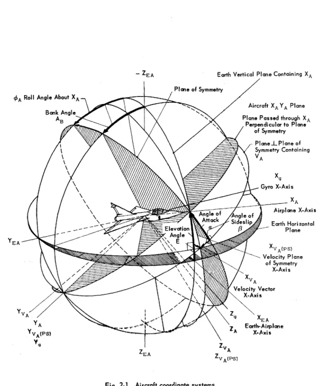
Figure 2-1 defines the coordinate systems that are used to orient the aircraft and its velocity vector with respect to the earth. Five orthogonal right-hand coordinate systems are defined:
(1) the aircraft coordinates, A; these are established by axes fixed to the
aircraft with XA an arbitrarily chosen longitudinal axis in the plane of symmetry positive forward; YA perpendicular to the plane of symmetry, positive along the right wing; ZA perpendicular to XA and YA, positive down.
- ZEA Earth Vertical Plane Containing XA
Plane of Symmetry
A Roll Angle About XA
Aircraft X YA Plane
Bank AngleAA
A Plane Passed through X
Perpendicular to Plane
of Symmetry
Plane.L Plane of
Symmetry Containing
XA
Angle of Angle of Airplane X-Axis Attack Sideslip Earth Horizontal
-Elevation J6 Plane Angle YEA E VA(PS) Velocity Plane of Symmetry X-Axis N
~
Velocity Vector VA X-Axis A Y _. A. wth-Airplane AA X.Axis VA(PS) .-- itnFriae E AA .A ZVdsPS)Fig, 2-1. Aircraft coordinate systems.
(2) the gyro-coordinates, g; these are established by axes fixed to the aircraft with X in the aircraft plane of symmetry and parallel to the roll gyro input axis, positive forward; Y perpendicular to the plane of symmetry, and
Z perpendicular to the other two axes and also parallel to the yaw gyro input
axis, positive down.
(3) the velocity or flight path coordinates, VA; these are established by
axes fixed to the velocity vector with XV parallel to the aircraft's velocity
A
vector, positive forward; YV perpendicular to XV in the projection plane
A A
passed through VA perpendicular to the aircraft plane of symmetry, and ZVA perpendicular to the other two axes, positive down.
(4) the earth-airplane coordinates, (EA); these are derived from the aircraft axes .and the horizontal plane such that XEA is the intersection of the earth horizontal plane and the vertical plane passed through XA, positive forward; YEA is perpendicular to XEA in the horizontal plane, and ZEA is perpendicular to the horizontal plane, positive down.
(5) the velocity-plane of symmetry coordinates, VA (PS); these are
established by axes which are the same as aircraft coordinate axes when the X-axis is taken along the projection of the velocity vector into the plane of symmetry.
Equations of Motion
The aircraft equations of motion are the linearized relations commonly used to express the aircraft's behavior during small deviations from trimmed flight. The aircraft axes are assumed to be coincident with the velocity coordinate system in trimmed steady-state flight. If both the trimmed angular velocity of the aircraft with respect to inertial space and the sideslip angle are zero, then W(IA)XA becomes the deviation in the roll angular velocity of the airplane with respect to inertial space from trimmed flight; W(IA) ZA becomes the deviation in the yaw angular velocity of the airplane with respect to inertial space from trimmed flight; PA becomes the airplane's sideslip angular deviation from trimmed flight. Also if the rotation of the earth is neglected, let
W(IA)XA =
W(EA)X A
(2-2)
W(IA)ZA = W(EA)ZA
Finally since all components of angular velocity will be measured with respect to inertial space (or the earth by Eq. (2-2), let
26
W(IA)XA = W(EA)X WX
)
(2-3)
W(IA)z = W(EA)zA = WZA
Since the gyro input axes do not in general coincide with the aircraft axes, the corresponding definitions for the angular velocity inputs to the roll and yaw gyros are
W(IG)X =
W(EG)X
X(2-4)
W(IG)z = (EG)zQ z
The equations of motion for the aircraft are then, Rolling Moment: [A(xx) ) p
(
C1 [(xz)) P + C Z A Csa [(qSb U) p] 2U0 Pjb Lu Z -P Yawing Moment: (2-5) [(IA(xz). + ( )C n]WXA p) Cn] WZ - C C, 8 + C r -L q (u' + qSb WZA a + f~r Side Force: (2-6)CLO Cos E) + mU CL sin EO mU
- *X WZA +[ U )P - C yp 3= C Ys,8
(2-7)
In addition there are the equations relating the inputs to the rate gyros to WXA and WZA and that of the rudder to its input command.
Rate Gyros:
The angle between the X-gyro input axis and the X-aircraft axis is
A - X ] which is written as A when no ambiguity results. Thus
W(rA)X W(IG)X X ~X A - W g (2-8)
W(IA)Z W(IG)Z = z = WX sin A. + Wz
Cos
Ag (2-9)Rudder Control:
(the dynamic effects of the rudder servo and the neglected).
The Signal-Flow Diagram for the Aircraft
Equations (2-5) through (2-10) can be rewritten construction of the signal-flow diagram as follows: Rolling Velocity: (from rolling moment equation)
WXA b C C. 8a a + IA(xz)
Yawing Velocity: (from yawing moment equation)
ZA = [ I Cn 8a + [ IAf))P +
_qSb 2 UO
Sideslip Angle: (fromn side force equation)
CL cos EO ImU 0
PA ( UP W (U)
qS
Roll Gyro:
rate gyros have been
in the form suitable for the
p +
(
C Wz + C (2-11) (b) C]
WX + CL sin E] P . Wz A+ CnpA + Ca r (2-12) Cy 8rBr (2-13) Yaw Gyro: Wx = A cos A - Wz, sin A, Wz= Wx sin A + Wz cos A. Rudder Angle: 8r - (RF)"C..[ 8i I + (RF)rrc[W X'r ]WX + Syd[w zsrl(
$rp
Wz)The coefficients of the terms in Eqs. (2-11) through (2-16) are functions of
p, and they define the transmittances of the signal paths. Thus,
Aileron Angle: Node 1
Rolling Velocity: Node 2
Wx = TI-28a + T3-2WEZ + T4 2PA
Yawing Velocity: Node 3
Wz A Ti.38a + T2- WxA + T 4-3 PA + T5-3 ar 27 (2-14) (2-15) (2-16) (2-17) (2-18)
T 3-2 T5_3T4-3 T3-4 T2.-3 Si de F T2-4 T 1--2 2 Ts-8 X_ Rolling Moments T4-2
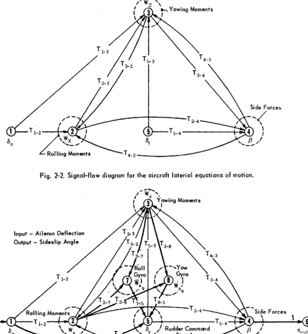
Fig. 2-2. Signal-flow diagram for the aircraft laterial equations of motion.
Yawing Moments
Input - Aileron Deflection T2-3
Output - Sideslip Angle T3- Ts-3 3-8
T3-7 T4-13 ~Rall - ,Yaw T-3 Gro I Gyro T--37 . 1 T -4 /_x W z T2-7 T2- T T8-5 7 2-4 Side Forces Rolling Moments - F -25 5-4
a / Rudder Command qO13
T4- 2
Fig. 2-3. Signal-flow diagram for aircraft rudder coordination system.
28
WZ Yawing Moments
T 3
T 1-3
Table 2-1. Definition of signal-flow path transmittances.
Q
Aileron Signal Paths Yaw Rate Signal Paths Rudder Signal Paths Derived TransmittancesT1 A( z)) p + (
)ct]
C. T-_ 1-T.4 T5 TS-4 T - T + T3-2T-4 T 2 T25 U7T75 +5T2-85 C-2 T1.- T+T3 T r- U CL sii T rj 4= - T2-- T-3 + T4-2T 3 __z___ - C T 4 - P [ P~J -- 3775+TT-- CgT 3 TT 3 3 + Ti-- T I T T T~~~T- - TRF T.S- T-4+ -' TL-. TT3 1-T23 T 1 -3 (f m 0 1 T S -4 A T 13 - T T- - cas A2 -T -TT I-3(Roll Rate Signal Paths
0
Sideslip Paths()
Rail Gyr Paths1T (Axz)- +( ec Cj- - (RF)rrc fw8 T-3 T T2-3 + T5
T3-T
-- I -
~
T3-2-1 1-3ZZ) - 1-3-]~
Rai Rat Sri Paths Sds® Yaw Gyro Paths I -3
T2 A c E0 T - T - +____ CIO__-S - d[z,8 ] T2-3 - T
[( ) - C
]
[( z -(-) -T 2 - I T + T2T-T27 = cos A E T' 3 - T2 3
T2- sin AT T32 - T T
Sideslip Angle: Node 4
PA 2-4 X A + T 3.4 W + T5.4ar (2-19)
Gyro Roll Rate: Node 7
WXg
= T2-7 WXA + T3-7 WZA (2-20)Gyro Yaw Rate: Node 8
W z = T2-8 WXA + T3-8WZA
(2-21)
Rudder Angle: Node 5
r = 1-5 a + T7-5 WX + T8-5 Wz (2-22)
Output: Node 6
q(Out) PA
The transmittances are summarized in Table 2-1.
These equations then result in the signal-flow diagram of Figs. 2-2 and
2-3. Figure 2-2 presents the signal-flow diagram for the aircraft lateral equations, and Fig. 2-3 results when the rudder coordination signal paths are added. Figure 2-3 can be reduced through the steps presented in Appendix A to obtain that of Fig. 2-4. The diagram can be further simplified if the side force due to rudder is negligibly small, and the diagram of Fig. 2-5 results. In this diagram there are two signal-flow paths to the sideslip node. These are the sideslip generated by the aircraft's rolling and yawing motions when the rudder is controlled in accordance with Eq. (2-16). In addition there is one self-generated closed loop at the sideslip node. This self-loop has the effect of dividing each of the transmittances of the signal paths entering the node by the quantity
[1 - (transmittance of the self-loop)]
However, the design objective of the rudder coordination system is to cause sideslip to be zero, and this then means that the sum of the signals entering the sideslip node is zero. Since the self-loop only affects the denominator of the sum of the signals, it can be eliminated as long as the system poles remain stable.
Thus Fig. 2-5 shows that the transmittances of the roll rate to rudder path and the aileron to rudder path must be chosen so that
T2-4Wx + T'' Wz =
o
(2-23)31 T z 3 T3-4 T1- 3 T2-3 0 1 T1-2 2-4
4
qn 8a TXq T4-4 T 1-4Fig. 2-4. Reduced signal-flow diagram for the rudder coordination system.
TS4 = 0 then TI-4 = 0 T3-4 T2-4 = T2 - 4 T"' T3-4 = T3-4 2-3 1-3 T3-4 = T3-4 + T3-2T2-4 4 1 6I Z -2 T'2- 4 = T24 8, WX TU T4-4
Fig. 2-5. Reduced signal-flow diagram for the rudder coordination system neglecting side force due to rudder.
32 or TI-2 T2-4 Sa + (T'i"3 + T12 T2-3) T' 4 ad = 0 (2-24) thus +(T"' + T 2T...) T"' 0 (2-25) T1-2 T2-4 + (T1-'3 + 1-2 2-3 3-4 =0( -5
Substituting the expressions of Table 2-1 for the primed quantities gives
+ T1 3 + TI.5 T5-3 + TI-2(T2-3 + T2 -T,3) x (T3.4 + T3-2T2 4) 0 (2-26)
[
1
- T3-3 - T3-2 (T2-3 + T2-5 T5-3) IThis equation can be further rewritten to obtain an expression relating the aileron to rudder coordination path, T1- 5, and the roll rate to rudder
coordina-tion path, T7-5, to the aircraft parameters. The general expression including
the effects of-climbing or diving flight is presented in Appendix C. When the aircraft is in level flight so that the elevation angle, E0, is zero, Eq. (2-26)
becomes
T
V. (
A(z)1/qSb)+
b Cn8 C 1U C) C I 26- C Cg C
Tn8
E
1+ A a 'A(xz) 0 n~ 8 a nSyd[WZ#8 ] r cos A 1 + (U1/g)(tan rr A) CP 1 A b(xx) Crib Sa + I x
g
b r Cn C T7 5 cos A - tan A]
UO U Cn C 8 C nrP U) PI-
C. p(
A(xx ) 2 b ) C, - I(,) \- _ p _ b C gr J ) qSb /[
\2U/ P \ qSb (UJ 2Ur
UI
(2-27)In Eq. (2-27), T7-5 is the relating function of the roll rate to rudder path and
T1-5 is the relating function of the aileron to rudder path. If one of these
relating functions is specified, Eq. (2-27) can then be solved for the relating function the second path must have if sideslip is to remain zero. Three special cases are of interest:
(a) when the rudder coordination system input is roll rate only, i. e. T1-5
(b) when input is aileron motion only, i. e. T7-5 0
(c) when both coordination paths are used, but the aileron to rudder
path is restricted to have the form S
1 + TP
These results in the relating functions given by Eqs. (2-28), (2-29), and (2-30) respectively. Case (a): (RF)rr[W 88rI = C~ T) ( A(z/qSb + a A s
1
U0
C r I Cia IA(zz)JCOS
Ag
bi C 1 C Sd[ ar 1 +(U./g)tan Ag 2U) C CI Cn Cos A. U0
(
IA(xx))[ Ca a x P C. ar Sb qb C c~e, cos A a I~v C \COScg/ nar a Cr Note: The component neglected. Case (b): (2-28)term (g/UO) tan A /p occurs in Eq. (2-27) due to the airplane yaw rate appearing as an input to the roll rate gyro. This term has been
(RF)ac 8 & I - T 1
-5 (2-29)
where T1-5 is given by Eq. (2-27) with T7-5 = 0
Case (c): T7 5
j
(IA(zz)/qSb) 0 C r b ( Cn [ a U C 0 Cn8r C1 +]
C IA(zz)]cos A. Cg (jS..ArW Ri
r]
1 -(UO/g) (tan A.)pSU 0 / z 1r 1 + rp I 33 (RF)rrc[wX, 8,r = (2-30a) p
_a AzA(xx) + a AI(xz) C \qSb C IAxx (RF)ac[W 8I T1 = 8 r ) C (IA(xx) (2-30b) A(xx) P + [-( -b _ A(xz) g qSb 2U, 0 qP
(neglecting the term
( C r U
For steady-state sideslip: use slow integration of sideslip or lateral acceleration. The expressions for these relating functions contain constants, lead-lag terms, ideal derivative and integral terms. The integral term primarily controls the
steady-state sideslip to provide the yawing moment required to balance the yawing moments due to yaw rate and due to the trim aileron deflection. In many high performance aircraft the steady-state sideslip is negligibly small. When this is not so, a slow acting integration of a direct measure of sideslip is better than an integration of roll rate.
For aircraft which do not exhibit a large yawing moment due to aileron, Cn , nor large products of inertia, the ideal derivative term can be neglected.
a
Thus coordination systems based upon either of the equations of Case (a) or Case (b) give excellent performance. If C is large however, the need for the
n6
the derivative term may be difficult to fulfill in Case (a). Similarly with Case (b) there is difficulty in balancing out the aileron signal voltage corresponding to trimmed flight so that there will not be a corresponding rudder deflection. Thus Case (c) is a combination of the other two cases in which the roll rate path is providing the constant and the lead-lag terms, while the aileron path provides the lead term in the form of a high-pass filter network and thereby avoids any
steady-state signal difficulties.
34
CHAPTER 3
DESIGN OF A CLOSED-LOOP SELF-ADJUSTING RUDDER
COORDINATION SYSTEM
Proper coordination of the rudder with the aileron to minimize transient sideslip can be obtained by feeding the rudder a command signal which is a function of the roll angular velocity as shown in Chapter 2. In the past this has
been done in a manner that was open-loop with respect to sideslip, and the per-formance depended upon a static calibration of the control path parameters. This chapter describes a method of providing closed-loop control to such a sys-tem so that the parameters will be automatically adjusted to minimize sideslip as flight conditions or the aircraft loading change.
The system under consideration is one in which only roll angular velocity is used for coordinating the rudder. The required relating function for the roll-rate to rudder control path is given by Eq. (2-28) of Chapter 2. This may be considered as the sum of four paths to the rudder: roll-rate direct, roll-rate through a lag, roll rate through a lead high-pass filter and roll rate through an
integration. It was assumed that the integration requirement was met by
integrating a measure of steady-state sideslip. Thus the system to be considered controls transient sideslip only.
Equation (2-28) shows that if the sensitivities of the direct, lag, and lead paths are properly adjusted, the transient sideslip is minimized. These sensitivities depend upon flight condition, the aircraft mass and aerodynamic parameters, and the characterisitics of the yaw damper loop. Therefore a system is required that will automatically adjust these sensitivities on the basis of a measure of the transient sideslip occurring during maneuvering flight.
Due to the difficulty in measuring sideslip directly, an effort was made to find another quantity which was easily measurable and which not only gave a unique indication of whether or not sideslip was zero, but also gave an unambiguous indication of whether the sensitivities were set too high or too low. Such a quantity has been found in the relationship which exists between the roll and yaw angular velocities during a perfectly coordinated turn (zero sideslip).
35
W(IA)Z
ZVA Component of Aircraft's
Angular Velocity with Respect to Inertial Space
ZVA
Roll Gyro
Input Axis Airc
Velo Vec A V W(IA)XV AA XVA Component of Ai Angular Velocity Respect to Inertial Yaw Gyro Input Axis -4-Xg raft city tor A so -- w VA rcraft's with Space Zg
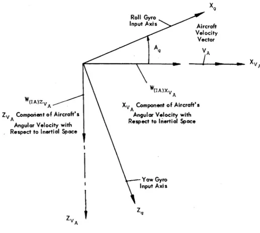
Fig. 3-1. Orientation of the gyro input axes relative to the velocity vector.
36
~1
Refer to Fig. 3-1:
If the components of the aircraft's angular velocity with respect to inertial space along the XVA and
ZVA axes are W(I^)XVA and W (IA)zV then the components of angular velocity measured by rate gyros whose input axes are rotated through the angle A[XVA.X = Ag from the velocity coordinate system are
(IA)X = W(IA)XVA cos Ag - (IA)ZVA (3-1)
(IA)Z g (IA)XVA sin A + W cos A (3-2)
For a constant altitude turn with zero sideslip,
W(IAg (.isin AB (3-3)
W(IA) ZA
B which can be approximated as
W(IA)z A (U)L (IA)XV (34)
VA \ UO/ P
Substitution of Eq. (3-4) into Eqs. (3-1) and (3-2) gives upon rearranging terms
(IA)X (IA)XVA Cos
(Az WAZg - W (IA)XV cos A + tan A (3-6)
g [U/ P
Eliminating W(IA)X A
S-
(
tan A (IA)Z = (tan AP W(IA)X (3-7)If Eq. (3-7) is multiplied by (rp/ I + rp),
( T AW + (U./g) (tan A ) p
U P (+ rp) W (IA )Z g U1 1 + rp
(3-Definition of an error quantity, (EQ)
(EQ)
( 7'P
)
W(IA)Zg - T9 r + /g) (tan A ) WA (3-9)\/ + rp
J
XThis expression neglects the term, (g/U0)(tan Ag/p), which is the yaw rate component sensed by the roll
rate gyro which is small compared with the total roll rate.
By the condition of Eq. (3-3), (EQ) is zero when sideslip is zero.
Derivation Summary 3-1.
Referring to Fig. 3-1, Derivation Summary 3-1 shows that when sideslip is zero the components of the angular velocity of the aircraft with respect to inertial space measured by the roll and yaw rate gyros are related by Eq. (3-7). Since this relation involves integral terms, it is more practical to use the relationship which results when the gyro outputs are filtered by high-pass filters. Neglecting for the purpose of this discussion that voltage signals would be involved with the physical equipment, there results the relation of Eq. (3-9) which defines an error quantity, (EQ).
(EQ) =
(p
W(IA)z -- i- [ + (U/g) (tn A.)P] W(IA)x (3-9)\Il+ rp/ ) UO /) I + rp J
Since Eq. (3-9) is true only when sideslip is zero, (EQ) will be zero when sideslip is zero and nonzero otherwise. (EQ) thus becomes a measure of how well the rudder coordination system is performing and can be used to change the parameters of the system so as to optimize that performance. The design of the self-adjusting system is based upon using the simple relationship defining
(EQ) as a control quantity.
Mechanization of the Error Quantity
In Chapter 2 it was shown that the ideal rudder coordination signal should include terms proportional, after suitable filtering, to the roll rate, rolling acceleration and roll angle. In many cases the predominant terms arise from the presence of the yaw rate damper added to damp the aircraft's natural lateral oscillation. Equation (2-28) of Chapter 2 presents the relating function of the rudder coordination system and shows that the term involving roll rate in the error quantity of Eq. (3-9) also appears as an important portion of the desired rudder coordination system's relating function. Thus the mechaniza-tion of the error quantity also furnishes a control signal for the rudder.
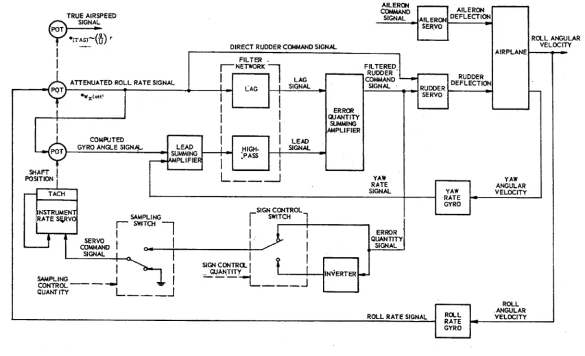
Figure 3-2 is a functional block diagram for a possible mechanization of the error quantity to control the rudder coordination system. (EQ) can be written
(EQ) -
2)
rw(IAZ, - ton A gW(IA)X r W(I A)X, (3-10)
Equation (3-10) shows that (EQ) can be computed by feeding'the yaw rate gyro signal through a high-pass filter and portions of the roll rate gyro signal through the same filter as well as through a lag filter. The poles of the two filters are identical and thus the same (RC) network can be used for both paths with the inputs entering at different points.
If the X-gyro axis is aligned with the aircraft's zero lift line, the angle Ag is equal to the aircraft's angle of attack, caA.
TRUE AIRSPEED SIGNAL
FILTER-F-NETWORK
ATTENUATED ROLL RARTE SIGNAL L
SIGICNTRL
COMPUTED LEAD
GYRO ANGLE SIGNAL- LEAD HIGH- SIGNAL
POT soSUMMING P ASS
SHAF APLIFIER
POSITION
TACH
NSTRUMENT SIGN CONTROL
RA TE SFRVO SAMPLING SWITCH
SWITCH SERVO COMMAND no SIGNAL SIGN CONTROL QUANTITY SAMPLING QUANT ITY - J AILERON COMMAND AILERON
SIGNAL AILERON DEFLECTION
SERVO FILTERED RUDDER RDE COMMAND R DEFLECTION SIGNAL RUDDER I SERVO YAW RATE SIGNAL ERROR QUANTITY SIGNAL INViERTER AIRPLANE YAW ANGULAR YAW VELOCITY RATE GYRO
ROLL RATE SIGNAL
ROLL .ANGULAR
ROLL VELOCITY
RATE -e GYRO
Fig. 3-2. Functional schematic diagram of rudder coordination system.
ROLL ANGULAR VELOCITY
DIRECT RUDDER COMMAND SIGNAL
ERROR
QUJANTITY
SUMMING
Thus,
tan A, tan a a (3-11)
But the angle of attack varies with flight condition as
(dC /da) P U2
20
or
GA=C (3-13)
0
where C varies with loading, slope of the lift curve, and altitude. If C were assumed to be constant, the sensitivity of the roll rate high-pass filter path would have to be varied with flight condition as (i/Uo)2 and therefore it would be proportional to the square of the sensitivity of the lag path. This relationship greatly simplifies the computing process since only one error quantity is then required rather than two to set the sensitivities of these two signal paths. The error quantity is therefore used to drive an instrument servo to position a shaft on which is mounted two potentiometers. By exciting one potentiometer with a roll rate signal its output determines the sensitivity of the lag path. By exciting the second pot by the output of the first pot, the output of the second pot determines the sensitivity of the lead-lag path.
The output of the second pot is combined with the yaw rate signal in a summing amplifier and fed to the filter network where all three signals are combined to form the error quantity. Since the terms forming the error quantity are also needed to control the rudder by Eq. (2-28) and to damp the lateral oscillation, the error quantity becomes one of the command paths to the rudder servo. To obtain the direct roll rate to rudder command path, the output of the first rudder coordination system pot is sent to the rudder servo. This approxi-mates the variation with flight condition of the direct roll rate path of Eq. (2-28). The error quantity is then sent through the sign control switch and the sampling switch to the potentiometer control instrument servo. The need for the sign con-trol switch can be seen from Eq. (3-9). If a turn is made to the right, both angular velocities will be positive. If the error quantity is positive, the value of (gT/U )
should be increased, i. e. the pot "turned up. " If (gT/U ) is set too low and a turn to the left is made, the error quantity will be negative but the pot value should still be increased. Thus the sign of signal sent to the instrument servo must be controlled by an indication of which way the aircraft is turning. The sign of the aileron deflection or the sign of the command input to the flight control system can be used as the sign control quantity.
Since the pot settings should be constant for a given flight condition, it is desirable to sample the error only as often as necessary and to leave the pot alone if it is set correctly. The control quantity for the sampling switch should thus be a quantity which indicates a maneuver is to take place. The aileron command signal or the command input to the flight control system are acceptable quantities to use. The disadvantage of using the command signal to the flight control system is that it restricts the pot adjustment to those times during which a command signal exists. In maneuvers such as dives, it may not be desirable to upset the system by putting in lateral command inputs. Thus the aileron may be the better sampling quantity.
CHAPTER 4
RESULTS OF THE SIMULATION STUDY
The performance of the automatic self-adjusting rudder coordination system designed in Chapter 3 was studied on a G. P. S. high speed analogue simulator.
The simulation set up is described in Appendix B. The ability of the system to coordinate the rudder with a simulated manual aileron input was examined first. This system is the same as that shown in Fig. 3-2. Later roll and yaw control loops were closed around this system so that the combined system became a completely automatic flight control system. The sensitivities of the outer control loops were assumed to be set in a manner independent of the rudder coordination system. In both cases it was assumed that yaw rate was fed to the rudder to damp the aircraft lateral oscillation.
Most of the study was done considering the system to be installed in an F-94A aircraft. The basic flight condition for comparison purposes was taken to be a Mach number of 0.6 at 22, 000 foot altitude. The parameter variations studied are listed in Table 4-1. A brief examination of the performance of the system when installed in an F-100A aircraft was also made.
For the manual aileron inputs and for the first flight control system studies, the error quantity was sampled only when there was an aileron deflection from trim that produced a signal large enough to actuate the sampling switch. In the later flight control system studies, the sampling switch was in continuous operation. Since the sign of the error changes with the direction of roll, the sign of the instrument servo command signal must be made independent of the direction of rolling so that the sensitivity variation would always be in the proper direction. The algebraic sign of the aileron deflection from trim was used to control the "sign switch. " For the case of the manual aileron inputs the aileron was deflected in only one direction, but in the case of the flight control system the sign of the aileron deflection changed whenever the system was oscillatory. Transient time responses of the system are presented in Figs. 4-1 through 4-5, which are photographs of the oscilloscope on which the simulator outputs are displayed. Each curve represents approximately 10 seconds of the response following the initiation of the input. At the end of each sweep (or about 10 second