Coarse “split and lump” bilingual language models for richer source information in SMT

Publisher’s version / Version de l'éditeur:

Proceedings of the Eleventh Conference of the Association for Machine

Translation in the Americas (AMTA), 2014, 1, pp. 28-41, 2014-10

READ THESE TERMS AND CONDITIONS CAREFULLY BEFORE USING THIS WEBSITE. https://nrc-publications.canada.ca/eng/copyright

Vous avez des questions? Nous pouvons vous aider. Pour communiquer directement avec un auteur, consultez la première page de la revue dans laquelle son article a été publié afin de trouver ses coordonnées. Si vous n’arrivez pas à les repérer, communiquez avec nous à PublicationsArchive-ArchivesPublications@nrc-cnrc.gc.ca.

Questions? Contact the NRC Publications Archive team at

PublicationsArchive-ArchivesPublications@nrc-cnrc.gc.ca. If you wish to email the authors directly, please see the first page of the publication for their contact information.

NRC Publications Archive

Archives des publications du CNRC

This publication could be one of several versions: author’s original, accepted manuscript or the publisher’s version. / La version de cette publication peut être l’une des suivantes : la version prépublication de l’auteur, la version acceptée du manuscrit ou la version de l’éditeur.

Access and use of this website and the material on it are subject to the Terms and Conditions set forth at

Coarse “split and lump” bilingual language models for richer source

information in SMT

Darlene, Stewart; Roland, Kuhn; Eric, Joanis; George, Forster

https://publications-cnrc.canada.ca/fra/droits

L’accès à ce site Web et l’utilisation de son contenu sont assujettis aux conditions présentées dans le site LISEZ CES CONDITIONS ATTENTIVEMENT AVANT D’UTILISER CE SITE WEB.

NRC Publications Record / Notice d'Archives des publications de CNRC:

Coarse “split and lump” bilingual language

models for richer source information in SMT

Darlene Stewart

Darlene.Stewart@nrc.gc.ca

Roland Kuhn

Roland.Kuhn@nrc.gc.ca

Eric Joanis

Eric.Joanis@nrc.gc.ca

George Foster*

George.Foster@nrc.gc.ca

All authors originally at: National Research Council, Ottawa, Canada K1A 0R6

* This author is now at Google Inc., Mountain View, California 94043

Abstract

Recently, there has been interest in automatically generated word classes for improving sta-tistical machine translation (SMT) quality: e.g, (Wuebker et al, 2013). We create new mod-els by replacing words with word classes in features applied during decoding; we call these “coarse models”. We find that coarse versions of the bilingual language models (biLMs) of (Niehues et al, 2011) yield larger BLEU gains than the original biLMs. BiLMs provide phrase-based systems with rich contextual information from the source sentence; because they have a large number of types, they suffer from data sparsity. Niehues et al (2011) miti-gated this problem by replacing source or target words with parts of speech (POSs). We vary their approach in two ways: by clustering words on the source or target side over a range of granularities (word clustering), and by clustering the bilingual units that make up biLMs (bitoken clustering). We find that loglinear combinations of the resulting coarse biLMs with each other and with coarse LMs (LMs based on word classes) yield even higher scores than single coarse models. When we add an appealing “generic” coarse configuration chosen on English > French devtest data to four language pairs (keeping the structure fixed, but providing language-pair-specific models for each pair), BLEU gains on blind test data against strong baselines averaged over 5 runs are +0.80 for English > French, +0.35 for French > English, +1.0 for Arabic > English, and +0.6 for Chinese > English.

1.

Introduction

This work aims to provide rich contextual information to phrase-based SMT, in order to miti-gate data sparsity. We cluster the basic units of the bilingual language model (biLM) of Niehues et al (2011) and of standard language models (LMs). A “generic”, symmetric config-uration chosen on English > French devtest yields BLEU gains over strong baselines on blind test data of +0.80 for English > French (henceforth “Eng>Fre”), +0.35 for French > English (“Fre>Eng”), +1.0 for Arabic > English (“Ara>Eng”), and +0.6 for Chinese > English (“Chi>Eng”). If we apply the configuration with the highest devtest score on a given language pair to blind data, the gains are +0.85 for Eng>Fre, +0.46 for Fre>Eng, and +1.2 for Ara>Eng, but still +0.6 for Chi>Eng.

1.1. Coarse bilingual language models (biLMs) for source context

Though coarse biLMs are the focus of this paper, we explored other coarse models: models where words are replaced by word classes. E.g., we obtained good gains in earlier experi-ments with coarse LMs. Since others have explored that terrain before us (see 1.2), this paper focuses on the “bilingual language model” (biLM) of Niehues et al (2011). In phrase-based

SMT, information from source words outside the current phrase pair is incorporated only indi-rectly, via target words that are translations of these source words, if the relevant target words are close enough to the current target word to affect LM scores. BiLMs address this by align-ing each target word in the trainalign-ing data with source words to create “bitokens”. An N-gram bitoken LM is then trained. A coarse biLM is one whose words and/or bitokens have been clustered into classes. Our best results were obtained by combining coarse biLMs with coarse LMs. We tune our system with batch lattice MIRA (Cherry and Foster, 2012), which supports loglinear combinations that have many features.

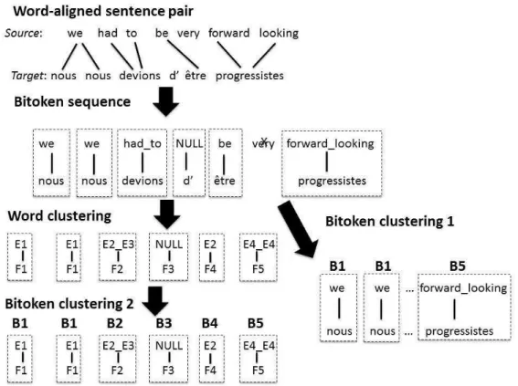
Figure 1 shows word-based and coarse biLMs for Eng>Fre. A target word and its aligned source words define a bitoken. Unaligned target words (e.g., French word “d’ ” in the example) are aligned with NULL. Unaligned source words (e.g., “very”) are dropped. A source word aligned with more than one target word (e.g., “we”, aligned with two instances of “nous”) is duplicated: each target word aligned with it receives a copy of that source word.

Figure 1. Creating bitokens & bitoken classes for a bilingual language model (biLM)

BiLMs can easily be incorporated into a phrase-based architecture. The decoder still uses phrase pairs from a phrase table to create hypotheses. However, a new LM with a wide context span of source information can now score hypotheses, along with the standard LM (Niehues et al found it was best to retain the latter). Unfortunately, the bitoken vocabulary of a biLM will be much bigger than the target-language vocabulary, because a target word is often split into different bitokens. E.g., the word “être” might be split into three bitokens: “être_be”, “être_being”, and “être_to-be”. One solution to the sparsity problem is to lump bitokens into new classes. E.g., one could replace each English or French word above with its part of speech (POS). In (Niehues et al, 2011), this “split and lump” process was applied to

both sides of a biLM for Ara>Eng SMT. When the biLM was added as a new loglinear fea-ture to a system with a word-based biLM, it yielded a modest gain of about +0.2 BLEU. In our work, we try other versions of “split and lump”. Instead of using taggers to define POSs, we use a program called mkcls (see 1.2) to create clusters. Unlike Niehues et al (2011), we vary the granularity of word clustering, and sometimes cluster the bitokens themselves, call-ing the resultcall-ing models “coarse biLMs”.

Figure 1 also shows three ways of building coarse biLMs: 1. clustering source and/or target words, then creating bitokens. 2. clustering the word-based bitokens themselves, with

mkcls using bitoken perplexity as its criterion (in Fig. 1, “bitoken clustering 1”). 3. clustering bitokens whose source and/or target words have been “preclustered” (“bitoken clustering 2”). Here, E1, E2, etc., and F1, F2, etc., are word classes generated by mkcls operating on source (English) and target (French) text respectively; B1, B2, etc. denote bitoken classes.

Figure 2. Two-pass construction of bitokens for a coarse biLM

Figure 2 illustrates the three types of coarse biLM, each shown by a dotted-line oval. A key aspect of a biLM is its bitoken vocabulary size. E.g., for the Eng>Fre experiments on which Figure 2 is based, the original word biLM had a vocabulary of 7.6 million bitokens. Coarse biLMs result from two passes of bitoken vocabulary compression, both optional: a first pass of clustering of source and/or target words, and a second pass of bitoken clustering. Skipping both passes yields the word-based biLM. The X coordinates in Figure 2 give the biLM vocabulary size after the first pass, and the Y coordinates give its size after the second pass (as a percentage of its original size). The original biLM (“word biLM”) is in the upper right-hand corner: both passes are null operations, so the coordinates are (100%,100%).

We denote word clustering by (n1, n2), where n1 and n2 are number of source and tar-get word classes respectively. |S| and |T| are the original sizes of the source and tartar-get vocabu-laries. The top oval in Figure 2 contains coarse biLMs obtained by pass 1 (word clustering) but not pass 2 (bitoken clustering). E.g., “(400, 200)” is the coarse biLM obtained by using 400 and 200 word classes for English and French respectively; “(1600, |T|)” is the coarse biLM obtained with 1600 English classes and no clustering for French. The oval on the far right contains biLMs created when only pass 2 is applied. E.g., “50 bi” is the coarse biLM obtained by clustering the 7.6M word-based bitokens down to only 50. The third oval con-tains coarse biLMs produced by applying pass 1, then pass 2. E.g., “400 bi(400,200)” is the coarse biLM obtained by creating bitokens with 400 and 200 source and target word classes respectively, then clustering these bitokens into 400 classes. A defect of the figure is that its axes don’t represent the difference between word clustering on the source vs. target sides. However, the figure conveys our greatest problem: the vast number of possible coarse biLMs

There is a big space in the middle of the figure that wasn’t explored in our experi-ments: there are no final biLMs that have between 0.01% and 10% of the original number of word biLMs, because mkcls becomes very slow as the number of word classes grows: creat-ing coarse biLMs like “(10,000, 10,000)” or “10,000 bi(400,400)” is infeasible.

1.2. Related work

This section will discuss work on coarse models, source-side contextual information for SMT, and lexical clustering techniques (including mkcls, used for our experiments).

Uszkoreit and Brant (2008) explored coarse LMs for SMT. Wuebker et al (2013) de-scribe coarse LMs, translation models (TMs), and reordering models (RMs). Best perfor-mance was obtained with a system containing both word-based and coarse models. Prior to our current work, we experimented with discriminative hierarchical RMs (DHRMs) (Cherry, 2013). These combine the hierarchical RM (HRM) of (Galley and Manning, 2008) with sparse features conditioned on word classes for phrases involved in reordering; word classes are obtained from mkcls. Like Cherry (2013), we found that DHRM outperformed the HRM version for Ara>Eng and Chi>Eng. However, experiments with English-French Hansard data showed only small gains for DHRM over HRM. Thus, while all the Ara>Eng and Chi>Eng experiments reported in this paper employ DHRM - a coarse reordering model - none of the Eng<>Fre experiments do. In prior experiments, we also studied coarse phrase translation

models, but unlike Wuebker et al (2013), we found they did not yield significant improve-ments to our system, except when there is little training data. Many experiimprove-ments in this paper involve coarse language models. These are particularly effective for morphologically rich languages (e.g., Ammar et al, 2013; Bisazza and Monz, 2014). In unpublished earlier experi-ments, we found that coarse LM combinations can yield better results than using just one.

Besides biLMs (Niehues et al, 2011), there are other ways of incorporating additional source-language information in SMT. These include spectral clustering for HMM-based SMT (Zhao, Xing and Waibel, 2005), stochastic finite state transducers based on bilingual ngrams (Casacuberta and Vidal, 2004; Mariño et al, 2006; Crego and Yvon, 2010; Zhang et al, 2013), the lexicalized approach of (Hasan et al, 2008), factored Markov backoff models (Feng et al, 2014) and the “operation sequence model” (OSD) of (Durrani et al, 2011 and 2014). (Durrani et al 2014) appeared after our current paper was submitted. Our work and theirs shares an underlying motivation in which mkcls is applied to make earlier models more powerful, though the OSD models and ours are very different. We chose to implement biLMs primarily because this is easy to do in a phrase-based system.

Automatic word clustering was described in (Jelinek, 1991; Brown et al, 1992). In “Brown” or “IBM” clustering, each word in vocabulary V initially defines a single class.

These classes are clustered bottom-up into a binary tree of classes, with classes iteratively merging to minimize text perplexity under a class-based bigram LM, until the desired number of classes C is attained. Martin, Liermann, and Ney (1998) describe “exchange” clustering. Each word in V is initially assigned to a single class in some fashion. Then, each word in turn is reassigned to a class so as to minimize perplexity; movement of words between classes continues until a stopping criterion is met. When these authors compared various word clus-tering methods, the perplexity results were almost identical. The lowest bigram perplexity is usually obtained when each of the most frequent words is in a different class; different word clustering methods typically all ended up with arrangements similar to this. These authors obtained their best perplexity and speech recognition results when the clustering criterion was based on trigrams as well as bigrams, but this makes clustering expensive. Och (1999) focuses on bilingual word clustering and discusses ideas similar to bitoken clustering, though not in the context of phrase-based SMT. Uszkoreit and Brant (2008) describe a highly efficient dis-tributed version of exchange clustering. Faruqui and Dyer (2013) propose a bilingual word clustering method whose objective function combines same-language and cross-language mutual information. Applied to named entity recognition (NER), this yields significant im-provements. Turian, Ratinov and Bengio (2010) apply Brown clustering to NER and chunk-ing. Finally, Blunsom and Cohn (2011) improve Brown clustering by using a Bayesian prior to smooth estimates, by incorporating trigrams, and by exploiting morphological information. For word clustering, we chose a widely used program, mkcls: Blunsom and Cohn (2011) note its strong performance. We could have used POSs, but they have definitions that vary across languages; mkcls can be applied in a uniform way (though with the disadvantage that it gives each word a fixed class, instead of several possible classes as with POSs). Niesler et al (1998) found that automatically derived word classes outperform POSs. Until recently, the only document describing mkcls was in German (Och, 1995): accurate English infor-mation was unavailable. It is often suggested that mkcls implements (Och, 1999), but this is only partly true. Fortunately, Dr. Chris Dyer now provides an accurate description on his blog: http://statmt.blogspot.ca/2014/07/understanding-mkcls.html. Basically, mkcls executes an ensemble of optimizers and merges their results; the criterion for all steps is minimal bi-gram perplexity. Dr. Dyer estimates that the perplexity of an LM built from the resulting word classes is typically 20-40% lower than for bottom-up Brown clustering on its own.

2.

Experiments

2.1. Experimental approach

Using four diverse large-scale machine translation tasks (Eng>Fre, Fre>Eng, Ara>Eng, Chi>Eng), we studied the impact of coarse BiLMs in isolation and in combination with coarse LMs. Our challenge was to explore the most interesting possibilities without doing innumera-ble experiments. Ammar et al (2013) note that coarse models are particularly effective when the target language has complex morphology. We thus decided to use Eng>Fre experiments on devtest data to carry out initial explorations: this language pair would be a sensitive one. Our metric was average BLEU over Devtest1 and Devtest2 for a Hansard system (see Table

1). There is insufficient space to report all these Eng>Fre devtest experiments. The first round of experiments made us decide to explore coarse LMs and coarse biLMs, but not coarse TMs (these only gave appreciable gains for small amounts of training data); we would employ Wit-ten-Bell smoothing for the coarse models (coarse models generate counts of counts that the SRILM implementation of Kneser-Ney can’t cope with, and Witten-Bell slightly outper-formed Good-Turing for coarse models); we would use 8-gram coarse models (results dif-fered only slightly along the range from 6-grams to grams, but were marginally better for

8-grams). We then began a second round of Eng>Fre experiments with the same devtest (see

2.4 and Table 4); the results informed all subsequent experiments.

2.2. Experimental data

For English-French experiments in both directions, we used the high-quality Hansard corpus of Canadian parliamentary proceedings from 2001-2009 (Foster et al, 2010). We reserved the most recent five documents (from December 2009) for development and testing material, and extracted the dev and test corpora shown in Table 1. Some of the documents were much larg-er than typical devtest sizes, so we sampled subsets of them for the dev and test sets.

Corpus # sentence pairs # words (English) # words (French)

Train 2.9M 60.5M 68.6M

Tune 2,002 40K 45K

Devtest1 2,148 43K 48K

Devtest2 2,166 45K 50K

Test1 (blind test) 1,975 39K 44K Test2 (blind test) 2,340 49K 55K

Table 1. Corpus sizes for English<>French Hansard data

For Ara>Eng and Chi>Eng, we used large-scale training conditions defined in the DARPA BOLT project; Tables 2 and 3 give statistics. For Arabic, “all” includes 15 genres and MSA/Egyptian/Levantine/untagged dialects; “small” is “all” minus UN data; “webforum” is the webforum subset of “small”. Tune, Test, and SysCombTune are webforum genre, and a similar dialect mix. For Chinese all training sets are mixed genre; “good” is “all” minus UN, HK, and ISI data; Tune, SysCombTune, and Test are forum genre. NIST Open MT 2012 test data was the held-out data: for Arabic it is a mix of weblog/newsgroup genres; for Chinese it contains these two genres plus unknown genre. In Tables 2 and 3, the number of English words for Tune, Devtest1, Devtest2, and Test is averaged over four references.

Corpus # sentence pairs # words (Arabic) # words (English)

Train1: “all” 8.5M 261.7M 207.5M Train2: “small” 2.1M 42.4M 37.2M Train3: “webforum” 92K 1.6M 1.8M Tune 4,147 66K 72K Devtest1: “Test” 2,453 37K 40K Devtest2: “SysCombTune” 2,175 35K 38K Test (blind): MT12 Arabic test 5,812 229K 209K

Table 2. Corpus sizes for tokenized Arabic-English data

Corpus # sentence pairs # words (Chinese) # words (English)

Train1: “all” 12M 234M 254M

Train2: “good” 1.5M 32M 38M

Tune 2,748 62K 77K

Devtest1: “Test” 1,224 29K 36K Devtest2: “SysCombTune” 1,429 31K 38K Test (blind): MT12 Chinese test 8,714 224K 261K

2.3. Experimental systems

Eng<>Fre Hansard experiments were performed with Portage, the National Research Council of Canada’s phrase-based system (this is the system described in Foster et al, 2013). The cor-pus was word-aligned with HMM and IBM2 models; the phrase table was the union of phrase pairs from these alignments, with a length limit of 7. We applied Kneser-Ney smoothing to find bidirectional conditional phrase pair estimates, and obtained bidirectional Zens-Ney lexi-cal estimates (Chen et al, 2011). Hierarchilexi-cal lexilexi-cal reordering (Galley and Manning, 2008) was used. Additional features included standard distortion and word penalties (2 features) and a 4-gram LM trained on the target side of the parallel data: 13 features in total. The decoder used cube pruning and a distortion limit of 7.

Our Chinese and Arabic baselines are strong phrase-based systems, similar to our en-tries in evaluations like NIST. The hierarchical lexical reordering model (HRM) of (Galley and Manning, 2008) along with the sparse reordering features of (Cherry, 2013) was used. Phrase extraction pools counts over symmetrized word alignments from IBM2, HMM, IBM4, Fastalign (Dyer et al, 2013), and forced leave-one-out phrase alignment; the HRM pools counts in the same way. Phrase tables were Kneser-Ney smoothed as for the Eng<>Fre exper-iments, and combined with mixture adaptation (Foster, 2007); indicator features tracked which extraction techniques produced each phrase. The Chinese system incorporated addi-tional adaptation features (Foster et al, 2013). For both Arabic and Chinese, four LMs per system were trained: one LM on the English Gigaword corpus (5-gram with Good-Turing smoothing), one LM on monolingual webforum data and two LMs trained on selected materi-al from the parmateri-allel corpora (4-gram with Kneser-Ney smoothing); in the case of Chinese, the latter two LMs were mixture-adapted.. Both systems used the sparse features of (Hopkins and May, 2011; Cherry, 2013). The decoder used cube pruning and a distortion limit of 8.

Tuning for all systems was performed with batch lattice MIRA (Cherry and Foster, 2012). The metric is the original IBM BLEU, with case-insensitive matching of n-grams up to n = 4. For all systems, we performed five random replications of parameter tuning (Clark et al, 2011).

For Eng<> Fre, coarse models were trained on all of “Train”. For Ara>Eng, word clas-ses and two static coarse LMs were trained on “all” and “webforum” (no linear mixing), but biLMs were trained on “small”. For Chi>Eng, word classes and a large static mix coarse LM were trained on “all”, but a smaller dynamic mix coarse LM and all the biLMs were trained on “good”. Bitokens for all language pairs were derived from word-aligned sentence pairs by two word alignment techniques. Two copies of each pair were made; one was aligned using HMMs, the other using IBM2. Since the Arabic and Chinese phrase tables were created not only with these alignment techniques, but with others, the decoder for these languages may use bitokens not found in the biLMs (“out-of-biLM-vocabulary” bitokens).

2.4. English > French experiments

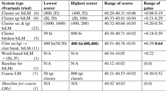
First, we explored single Eng>Fre coarse models on devtest data. For models involving word classes, we looked at 50, 100, 200, 400, 800, and 1600 classes. The number of bitoken types was huge (7.6M), so we were only able to obtain up to 800 bitoken classes (generating 1600 classes would have taken too long). There is insufficient space to show all results: Table 4 shows how many variants of each coarse model type we tried, along with the lowest-scoring and highest-scoring variant of each type (using average score on Devtest1 and Devtest2). The table uses the notation for biLMs given towards the end of section 1.1. The range of scores from lowest to highest is shown with the standard deviation (SD) over five tuning runs (more precisely, we show whichever is greater, the SD of the lowest or of the highest score).

System type (#variants tried)

Lowest scorer

Highest scorer Range of scores Range of gains Cluster src biLM (6) (800, |T|) (400, |T|) 40.20-40.31 ±0.06 +0.08-0.19 Cluster tgt biLM (6) (|S|, 50) (|S|, 100) 40.33-40.41 ±0.04 +0.21-0.29 Cluster src & tgt biLM (22) (1600, 1600) (400, 200) 40.32-40.66 ±0.05 +0.20-0.54 Cluster bitoken biLM (5) 50 bi 800 bi 40.30-40.71 ±0.02 +0.18-0.59 Clstr src/tgt → clstr bitok. biLM (11) 400 bi(50,50) 400 bi(400,400) 40.51-40.76 ±0.01 +0.39-0.64 Word-based biLM = (|S|, |T) (1) N/A N/A 40.34 ±0.05 +0.22 Baseline for biLMs (1) N/A N/A 40.12 ±0.02 (0.0) Coarse LM (7) 50 tgt classes 800 tgt classes 40.31-40.53 ±0.02 +0.30-0.52 (Baseline for coarse

LMs) (1)

N/A N/A 40.02 ±0.03 (0.0)

Table 4. Preliminary experiments - Eng>Fre average(Devtest1,Devtest2) BLEU for single coarse models

We did not try all 36 combinations of source and target word clusters, but explored along the “diagonal” where the number of classes is the same for both sides: i.e., we tried (50, 50), … , (1600, 1600). Then we tried coarse biLMs in the neighbourhood of the best diagonal ones, eventually trying 22 different biLMs clustered on both sides. For bitoken clustering, we also carried out this kind of greedy search. Word preclustering shortens the time required for bitoken clustering. E.g., on our machines, training the highest-scoring biLM, 400 bi(400,400), took 19 hours for (400,400) preclustering and then 112 hours for bitoken clustering: 131 hours total. Training “400 bi” with no preclustering took 277 hours. The shorter time with precluste-ring is because mkcls takes time proportional to the number of types: 7.6M bitokens without preclustering but only 3.2M with (400, 400) preclustering. Table 4 shows that preclustering followed by bitoken clustering also yielded the best results: the worst-scoring biLM of this type performed about +0.4 better than the baseline, and the best-performing one gained more than +0.6.The last two rows of the table pertain to coarse LMs. The Table 4 experiments were performed two months earlier than the rest, with a slightly different version of the system, one with a standard rather than hierarchical lexicalized reordering model (HRM) (tables 5 & 6 below show results with HRMs, and tables 7 & 8 with discriminative HRMs (DHRMs)).

Next, we explored loglinear combinations of the highest-scoring coarse models on the same devtest, again doing a kind of greedy search (and using HRMs). Because of the poor results for clustering on only source or target words (not both) in Table 4, we did not try these biLMs in combinations. Almost all the combinations we tried scored significantly higher than the coarse models of which they were composed, as shown in Table 5 (in descending order of devtest score). A pattern emerged: many of the highest-scoring combinations had one coarse biLM with clustered bitokens (sometimes preclustered, sometimes not), one coarse biLM with clustered source and target words, and two or three coarse LMs of very different granularity. Presumably, these information sources complement each other. We chose one of the configu-rations that scored highest on Eng>Fre devtest to be tried on all four language pairs – in each case, keeping the structure but using language-pair-specific models. This “generic” configura-tion often scores lower for other language pairs on blind test data than combinaconfigura-tions that have

been chosen via experiments on devtest data for a given pair, but is a reasonable choice for system builders who don’t wish to spend a lot of time on preliminary experiments.

In addition to “generic” (underlined) and the two other best combinations, Table 5 shows individual models inside coarse model combinations (in italics), the word-based biLM, and the baseline (the notation here was defined in section 1.1 above). Average scores and standard deviations from five runs are shown. For individual biLMs, “|B|” is the number of bitoken types. E.g., clustering English and French words to 400 and 200 classes respectively shrinks the number of different bitokens from 7.6 million to 2.9 million. Results on blind test data (Test1 and Test2) are lower than on devtest but in roughly the same order; coarse model combinations score higher than their components on both devtest and test data. The “generic” configuration we chose was the one with symmetric biLMs (no difference between number of source and target word classes in its biLMs) that scores highest on devtest. It has a biLM clus-tered to 400 classes for each language, a biLM obtained from the former by clustering it to 400 bitokens, and two coarse LMs of very different granularities (100 and 1600 classes).

Table 5. Eng>Fre BLEU for coarse model combinations (single components in italics)

2.5. Experiments with other language pairs

Experiments with the other language pairs were carried out as with Eng>Fre: greedy search over single coarse models followed by greedy search over model combinations, using scores on devtest for each pair to make decisions. Results on devtest and blind test data are shown in

Tables 6 – 8 for the two combinations scoring highest on devtest for each pair. For each pair,

we also tested the “generic” configuration (underlined) chosen on the basis of Eng>Fre devtest results. All results shown are averaged over 5 tuning runs.

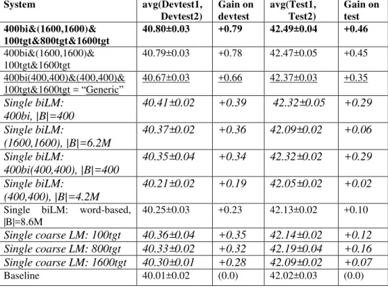
System avg(Devtest1, Devtest2) Gain on devtest avg(Test1, Test2) Gain on test 400bi(400,400)&(400,200)& 100tgt&1600tgt 41.25±0.03 +1.13 42.64±0.02 +0.85 400bi(400,400)&(400,400)& 100tgt&1600tgt = “Generic” 41.19±0.01 +1.07 42.59±0.03 +0.80 200bi&(400,200)& 100tgt&1600tgt 41.19±0.02 +1.07 42.60±0.04 +0.81 Single biLM: 400bi400src400tgt, |B|=400 40.76±0.01 +0.64 42.22±0.02 +0.43 Single biLM: 200 bi, |B|=200 40.69±0.03 +0.57 42.08±0.03 +0.28 Single biLM: (400,200), |B|=2.9M 40.66±0.02 +0.54 42.17±0.01 +0.37 Single biLM: (400,400), |B|=3.2M 40.51±0.04 +0.39 42.15±0.03 +0.36 Single biLM: word-based, |B|=7.6M 40.34±0.05 +0.22 41.96±0.01 +0.17 Single coarse LM: 1600tgt 40.67±0.03 +0.55 42.36±0.03 +0.56 Single coarse LM: 100tgt 40.61±0.03 +0.49 42.11±0.02 +0.32 Baseline 40.12±0.02 (0.0) 41.79±0.02 (0.0)

System avg(Devtest1, Devtest2) Gain on devtest avg(Test1, Test2) Gain on test 400bi&(1600,1600)& 100tgt&800tgt&1600tgt 40.80±0.03 +0.79 42.49±0.04 +0.46 400bi&(1600,1600)& 100tgt&1600tgt 40.79±0.03 +0.78 42.47±0.05 +0.45 400bi(400,400)&(400,400)& 100tgt&1600tgt = “Generic” 40.67±0.03 +0.66 42.37±0.03 +0.35

Single biLM:

400bi, |B|=400

40.41±0.02

+0.39

42.32±0.05

+0.29

Single biLM:

(1600,1600), |B|=6.2M

40.37±0.02

+0.36

42.09±0.02

+0.06

Single biLM:

400bi(400,400), |B|=400

40.35±0.04

+0.34

42.32±0.02

+0.29

Single biLM:

(400,400), |B|=4.2M

40.21±0.02

+0.19

42.05±0.02

+0.02

Single biLM: word-based, |B|=8.6M 40.25±0.03 +0.23 42.13±0.02 +0.10

Single coarse LM: 100tgt

40.36±0.04

+0.35

42.14±0.02

+0.12

Single coarse LM: 800tgt

40.33±0.02

+0.32

42.19±0.04

+0.16

Single coarse LM: 1600tgt

40.30±0.01

+0.28

42.09±0.02

+0.07

Table 6. Fre>Eng BLEU for coarse model combinations (single components in italics)

3.

Discussion and Future Work

BiLMs provide phrase-based SMT systems with richer source-side context during decoding. In experiments with highly competitive baselines, pure word-based 8-gram biLMs yield only modest gains in the range +0.1–0.2 BLEU for four language pairs. This is probably due to training data sparsity caused by the large number of bitoken types. Indeed, when we replace word-based 8-gram biLMs with coarse 8-gram biLMs, we get much greater gains from the latter. Our results also show that coarse biLMs and coarse LMs of different granularities con-tain partially complementary information: for each of the language pairs, loglinear combina-tions of coarse models score higher than single coarse models on blind test data.

We defined a “generic” coarse configuration by looking at Eng>Fre devtest results: 400bi(400,400)&(400,400)&100tgt&1600tgt (a loglinear combination of two types of coarse biLM and two coarse LMs of very different granularities). For this configuration, BLEU gains over language-specific baselines on blind data were +0.80 for Eng>Fre, +0.35 for Fre>Eng,

+1.0 for Ara>Eng, and +0.6for Chi>Eng. If we apply the configuration with the highest dev-test score on a given language pair to blind data, the gains are +0.85 for Eng>Fre, +0.46 for Fre>Eng, +1.2 for Ara>Eng, and still +0.6 for Chi>Eng. The consensus in the literature is that coarse models help most when the target language has complex morphology, so we expected the largest gains to be for Eng>Fre: we were surprised by the large gains for Ara>Eng. It looks as though source context information is especially valuable for Ara>Eng.

The Eng>Fre baseline system’s LM took only 0.1G of storage, but adding the “gene-ric” coarse LM-biLM configuration brought this to 2.4G. Adding “gene“gene-ric” took Fre>Eng LM size from 0.1G to 2.0G. Because they have four LMs, baselines for the other two language

pairs have much higher total LM sizes than the Eng<>Fre baselines: adding “generic” took total LM size from 15.0G to 18.4G for Ara>Eng, and from 7.6G to 11.0G for Chi>Eng. We didn’t measure time or virtual memory (VM) during decoding impacts precisely: very roughly, adding “generic” increased decoding time about 30% for all four systems, and in-creased VM size about 60% for the Eng<>Fre systems and about 20% for the other two.

System avg(Devtest1, Devtest2) Gain on devtest Test Gain on test 400bi&(1600,1600)& 100tgt&1600tgt 40.56±0.09 +0.76 46.03±0.07 +1.20 400bi(800,800)& 100tgt&1600tgt 40.51±0.12 +0.72 45.74±0.13 +0.91 400bi(400,400)&(400,400)& 100tgt&1600tgt = “Generic” 40.43 ±0.08 +0.63 45.80±0.14 +0.97 Single biLM: 400bi, |B|=400 40.38±0.13 +0.59 45.43±0.07 +0.60 Single biLM: 400bi(800,800), |B|=400 40.23±0.04 +0.44 45.35±0.08 +0.52 Single biLM: 400bi(400,400), |B|=400 40.18±0.09 +0.38 44.94±0.18 +0.11 Single biLM: (400,400), |B|=1.2M 40.15±0.08 +0.36 45.02±0.07 +0.19 Single biLM: (1600,1600), |B|=2.1M 40.03±0.04 +0.23 45.10±0.12 +0.27 Single biLM: word-based, |B|=4.0M 40.06±0.06 +0.26 44.96±0.09 +0.13 Single coarse LM: 1600tgt 40.14±0.06 +0.34 45.12±0.09 +0.29 Single coarse LM: 100tgt 40.03±0.04 +0.23 45.10±0.05 +0.27 Baseline 39.80±0.05 (0.0) 44.83±0.08 (0.0)

Table 7. Ara>Eng BLEU for coarse model combinations (single components in italics)

There are several directions for future work:

 The method for hard-clustering words/bitokens could be improved – e.g.., as in Blunsom and Cohn (2011). As a reviewer helpfully pointed out, coarse models of the same type but different granularities could be trained more effi-ciently with true IBM clustering (Brown et al, 1992) to create a hierarchy for words or bitokens that would yield many different granularities after a single run, rather than by running mkcls several times (once per granularity).  Coarse models could be used for domain adaptation - e.g., via mixture models

that combine in-domain and out-of-domain or general-domain data (Koehn and Schroeder, 2007; Foster and Kuhn, 2007; Sennrich, 2012). In-domain sta-tistics will be better-estimated in a coarse mixture than in a word-based one.  “Mirror-image” word-based or coarse target-to-source biLMs could be used

to rescore N-best lists or lattices. If there has been word reordering, these would apply context information not seen during decoding. E.g., let source “A B C D E F G H” generate hypothesis “a b f h g c d e”, and “A” be aligned with “a”, “B” with “b”, etc. With trigram word-based biLMs, the trigrams in-volving “f” seen during decoding are “a_A b_B f_F”, “b_B f_F h_H”, and “f_F h_H g_G”. During mirror-image rescoring, the biLM trigrams involving

“f” that are consulted are “D_d E_e F_f”, “E_e F_f G_g”, and “F_f G_g H_h” – a different set of trigrams, potentially containing additional information.  In this work, the most time-consuming task was finding the best combination

of coarse models for a given language pair/corpus. We hope to devise a com-putationally cheap way of finding the best combination on devtest data. An approach based on minimizing the perplexity of held-out data might work, if the correlation between this and SMT quality turns out to be sufficiently high. An interesting direction for future work is comparison between coarse models and neural net (NN) approaches. In principle, everything learned by coarse LMs or coarse biLMs could be learned by a neural net (NN) trained on the same data. Will NNs make coarse mod-els obsolete? Only thorough experimentation will show which of NNs or coarse model com-binations really yield better translations – perhaps they complement each other. Currently, an advantage of coarse models over NNs is quicker training times; one could further shrink train-ing time for coarse models by incrementally adaptattrain-ing word clustertrain-ings trained on generic data to new domains. However, incremental adaptation is also a possible strategy for NNs. Analysis of these tradeoffs between coarse models and NNs – in terms of model quality, speed of training, ease of incremental adaptation, etc. – is our top priority for future work.

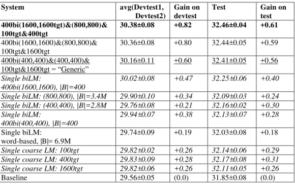
System avg(Devtest1, Devtest2) Gain on devtest Test Gain on test 400bi(1600,1600tgt)&(800,800)& 100tgt&400tgt 30.38±0.08 +0.82 32.46±0.04 +0.61 400bi(1600,1600)&(800,800)& 100tgt&1600tgt 30.36±0.08 +0.80 32.44±0.05 +0.59 400bi(400,400)&(400,400)& 100tgt&1600tgt = “Generic” 30.16±0.11 +0.60 32.41±0.05 +0.56 Single biLM: 400bi(1600,1600), |B|=400 30.02±0.08 +0.47 32.25±0.06 +0.40 Single biLM: (800,800), |B|=3.4M 29.90±0.10 +0.34 32.09±0.03 +0.24 Single biLM: (400,400), |B|=2.8M 29.76±0.08 +0.21 32.16±0.02 +0.30 Single biLM: 400bi(400,400), |B|=400 29.94±0.07 +0.38 32.13±0.07 +0.28 Single biLM: word-based, |B|= 6.9M 29.74±0.09 +0.19 32.03±0.08 +0.18 Single coarse LM: 100tgt 29.82±0.02 +0.26 32.14±0.06 +0.29 Single coarse LM: 400tgt 29.83±0.09 +0.28 32.17±0.08 +0.31 Single coarse LM: 1600tgt 29.82±0.06 +0.26 32.11±0.05 +0.26 Baseline 29.56±0.05 (0.0) 31.85±0.08 (0.0)

Table 8. Chi>Eng BLEU for coarse model combinations (single components in italic)

Acknowledgement

This research was supported in part by DARPA contract HR0011-12-C-0014 under subcon-tract to Raytheon BBN Technologies.

References

W. Ammar, V. Chahuneau, M. Denkowski, et al. 2013. The CMU Machine Translation Systems at WMT 2013. In Proceedings of Workshop on SMT, Sofia, Bulgaria.

A. Bisazza and C. Monz. 2014. Class-Based Language Modeling for Translating into Morphologically Rich Languages. In COLING, Dublin, Ireland.

P. Blunsom and T. Cohn. 2011. A Hierarchical Pitman-Yor Process HMM for Unsupervised Part of Speech Induction. In Proceedings of the ACL, Portland, Oregon, USA.

P. Brown, V. Della Pietra, P. de Souza, J. Lai and R. Mercer. 1992. Class based n-gram models of natu-ral language. Computational Linguistics, Vol. 18.

F. Casacuberta and E. Vidal. 2004. Machine Translation with Inferred Stochastic Finite-State Transduc-ers. Computational Linguistics. Vol. 30.

B. Chen, R. Kuhn, G. Foster and H. Johnson. 2011. Unpacking and transforming feature functions: New ways to smooth phrase tables. In Proceedings of MT Summit XIII, Xiamen, China.

C. Cherry. 2013. Improved reordering for phrase-based translation using sparse features. In Proceedings

of NAACL-HLT, Atlanta, USA.

C. Cherry and G. Foster. 2012. Batch Tuning Strategies for Statistical Machine Translation. In

Proceed-ings of NAACL-HLT, Montreal, Canada.

J. Clark, C. Dyer, A. Lavie and N. Smith. 2011. Better hypothesis testing for statistical machine transla-tion. In Proceedings of the ACL, Portland, Oregon, USA.

J. Crego and F. Yvon. 2010. Factored bilingual n-gram language models for statistical machine transla-tion. Machine Translation - Special Issue: Pushing the frontiers of SMT, V. 24, no. 2.

N. Durrani, H. Schmid, A. Fraser, and P. Koehn. 2014. Investigating the Usefulness of Generalized-Word Representations in SMT. In Proceedings of COLING, Dublin, Ireland.

N. Durrani, H. Schmid, and A. Fraser. 2011. A Joint Sequence Translation Model with Integrated Reor-dering. In Proceedings of the ACL, Portland, Oregon, USA.

C. Dyer, V. Chahuneau, and N. Smith. 2013. A Simple, Fast, and Effective Reparameterization of IBM Model 2. In Proceedings of NAACL, Atlanta, USA.

M. Faruqui and C. Dyer. 2013. An Information Theoretic Approach to Bilingual Word Clustering. In

Proceedings of the ACL, Sofia, Bulgaria.

Y. Feng, T. Cohn, X. Du. 2014. Factored Markov Translation with Robust Modeling. Proceedings of

CoNLL, Baltimore, USA.

G. Foster, B. Chen, and R. Kuhn. 2013. Simulating Discriminative Training for Linear Mixture Adapta-tion in SMT. In Proceedings of MT Summit, Nice, France.

G. Foster, P. Isabelle and R. Kuhn. 2010. Translating structured documents. In Proceedings of AMTA, Denver, USA.

G. Foster and R. Kuhn. 2007. Mixture-Model Adaptation for SMT. In Proceedings of Workshop on

M. Galley and C. Manning. 2008. A simple and effective hierarchical phrase reordering model. In

Pro-ceedings of EMNLP, Honolulu, USA.

S. Hasan, J. Ganitkevitch, H. Ney, and J. Andrés-Ferrer. 2008. Triplet Lexicon Models for Statistical Machine Translation. In Proceedings of EMNLP, Honolulu, USA.

M. Hopkins and J. May. 2011. Tuning as Ranking. In Proceedings of EMNLP, Edinburgh, Scotland. P. Koehn and J. Schroeder. 2007. Experiments in domain adaptation for statistical machine translation.

In Proceedings of Workshop on SMT, Prague, Czech Republic.

J. Mariño, R. Banchs, J. Crego, A. de Gispert, P. Lambert, J. Fonollosa, and M. Costa-jussà. 2006. N-gram-based machine translation. Computational Linguistics, Vol. 32, No. 4.

S. Martin, J. Liermann and H. Ney. 1998. Algorithms for bigram and trigram word clustering. Speech

Communication, Vol. 24.

J. Niehues, T. Herrmann, S. Vogel and A. Waibel. 2011. Wider Context by Using Bilingual Language Models in Machine Translation. In Proceedings of Workshop on SMT, Edinburgh, Scotland. T. Niesler, E. Whittaker, and P. Woodland. 1998. Comparison of POS and automatically derived

catego-ry-based LMs for speech recognition. In Proceedings of ICASSP, Vol. 1, Seattle, USA. F. Och. 1999. An efficient method for determining bilingual word classes. In Proceedings of EACL,

Stroudsburg, USA.

F. Och. 1995. Maximum-Likelihood-Schätzung von Wortkategorien mit Verfahren der kombina-torischen Optimierung. Studienarbeit (Master’s Thesis), University of Erlangen, Germany. R. Sennrich. 2012. Perplexity minimization for translation model domain adaptation in statistical

ma-chine translation. In Proceedings of EACL, Avignon, France.

J. Turian, L. Ratinov and Y. Bengio. 2010. Word representations: a simple and general method for semi-supervised learning. In Proceedings of ACL, Uppsala, Sweden.

J. Uszkoreit and T. Brants. 2008. Distributed word clustering for large scale class-based language mod-eling in machine translation. In Proceedings of ACL-HLT, Columbus, USA.

J. Wuebker, S. Peitz, F. Rietig and H. Ney. 2013. Improving Statistical Machine Translation withWord Class Models. In Proceedings of EMNLP, Seattle, USA.

H. Zhang, K. Toutanova, C. Quirk, and J. Gao. 2013. Beyond Left-to-Right: Multiple Decomposition Structures for SMT. In Proceedings of NAACL, Atlanta, USA.

B. Zhao, E. Xing, and A. Waibel. 2005. Bilingual Word Spectral Clustering for SMT. Proceedings of