Design of a demand driven multi-item-multi-stage manufacturing system : production scheduling, WIP control and Kanban implementation

(1)

Design of a Demand Driven Multi-Item-Multi-Stage

Manufacturing System: Production Scheduling,

WIP Control and Kanban Implementation

by

Xiaoyu Zhou

B.Eng., Mechanical Engineering and Automation Shanghai Jiao Tong University, 2008

MASSACHUSETTS INSETI"TE OF TECHNOLOGY

DEC 2 8 2009

LIBRARIES

SUBMITTED TO THE DEPARTMENT OF MECHANICAL ENGINEERING IN PARTIAL FULFILLMENT OF THE REQUIREMENTS FOR THE DEGREE OF

MASTER OF ENGINEERING IN MANUFACTURING AT THE

MASSACHUSETTS INSTITUTE OF TECHNOLOGY SEPTEMBER 2009

Signature of Author ...

- _- ^. A

Design of a Demand Driven Multi-Item-Multi-Stage

Manufacturing System: Production Scheduling,

WIP Control and Kanban Implementation

by Xiaoyu Zhou

Submitted to the Department of Mechanical Engineering on August 19, 2009 in Partial Fulfillment of the Requirements for the Degree of Master of Engineering in

Manufacturing

Abstract

The project is conducted in a multi-item-multi-stage manufacturing system with high volume products. The objectives are to optimize the inventory structure and improve production scheduling process. The stock building plan is studied carefully to understand the demand seasonality characteristics and the planning guidelines that the factory is currently following. A new base stock policy is introduced to the 5 focused production stages to establish a demand driven system with controlled inventory and new rules to guide the daily production. The line coupling concept is also added to further refine the inventory structure. After that, the production leveling method is employed to help reduce the variation of daily production targets. Finally, a Kanban system is designed to facilitate the demand driven manufacturing under the operation of the new base stock policy.

With the appropriate inventory control and production scheduling policy, the overall inventory level in the factory is reduced by 61% based on calculation, leading to a savings of 70% of the total inventory cost. Moreover, the establishment of Kanban system has simplified the daily manufacturing activity on the operation level and helped the factory become a lean manufacturer.

(3)

Disclaimer: The content of the thesis is modified to protect the real identity of the project

company. Company name and confidential information are omitted or disguised. Thesis Supervisor: Stanley B. Gershwin

(4)

Acknowledgement

First and foremost, the author wants to thank his thesis supervisor, Dr. Stanley B. Gershwin for his professional guidance and explanation throughout the course of the project. The discussions with him have provided the author with new perspectives when looking at the problems indentified, and have kept the project running on the right track.

Special thanks will be given to Prof. Stephen C. Graves, for his timely feedback and generous advices in helping the project team understand and implement his previous research work. The author would also like to thank Dr. Brian W. Anthony, for his effort in frequent travelling to Singapore and arranging project update meetings. Coming to professional writing, Mrs. Jennifer L. Craig has been extremely helpful in teaching the author how to write his first English thesis and giving invaluable comments and suggestions.

At the company side, sincere thanks are given to Mr. Yan Mun Tjun, my project supervisor. Being a senior operation manager, his constant support and commitment greatly facilitated the progress of the project. His dedication to implementing the project work encouraged the team to achieve a higher level of excellence. Many thanks are extended to other company colleagues, especially Mr. Tai Soon Wah, Mrs. Ng Ah Soon, Mr. Fong Ying Chuen and Mr. Lee Chee Teck. Sharing the same goal of making a better factory, the entire company personnel have provided the author a friendly and inspiring environment for investigation and discussion.

Finally, the author must thank his project teammates who worked together with him for 8 months, and provided him with constant support. They have always been generous with advice on the research work.

(5)

Table of Contents

List of Figures

Figure 1 Product Tree for PDAP Factory ... ... 12

Figure 2 Production Process Flow ... .... ... 13

Figure 3 Production Planning Process ... 15

Figure 4 Current Production Planning ... 18

Figure 5 Author's Focused Area... ... ... 20

Figure 6 Project Roadm ap ... 27

Figure 7 Procedures of Seasonality Analysis... 29

Figure 8 High Runner Selection & Daily Demand Pattern for Individual SKU... 31

Figure 9 Objectives of Production Leveling ... 32

Figure 10 Leveling Procedure in Excel Solver ... ... 34

Figure 11 Shipment Lead Time ... ... ... 35

Figure 12 Optimized Excel Solver Method ... ... 35

Figure 13 Objective of Line Coupling ... ... ... 41

Figure 14 Process Flow for SKUs: BA-HV and BA-SS ... ... 43

Figure 15 2009 PDAP Stock Building Plan ... ... 46

Figure 16 F-Values from Grouping 1, 2, 3 and 4... ... 47

Figure 17 P-Values from Grouping 1, 2, 3 and 4... ... 48

Figure 18 Confirmed Demand Pattern for SKU: DY-MRGL... ... 53

Figure 19 Leveled Production Targets from Monday to Tuesday ... ... 54

Figure 20 Leveled Production Targets from Monday to Sunday... ... 55

Figure 21 Daily Demand and Planned Production...56

Figure 22 Demand and Planned Production Targets in 120 days ... ... 56

Figure 23 Cumulative Demand vs. Cumulative Production for DY-MRGL ... 58

Figure 24 Daily Demand vs. Daily Production for DY-MRGL... ... 59

Figure 25 Reduction in C.V. after Excel Solver Method ... ... 60

(9)

List of Figures

Figure 26 Over Production on Day 7 ... ... ... ... 62

Figure 27 Leveling Effect under Different Leveling Methods ... 62

Figure 28 Comparison of Different Methods... 63

Figure 29 Summary of Reduction in C.V. (modify the picture) ... ... 65

Figure 30 Base Stock Levels in Production Stage 7 ... ... 69

Figure 32 Base Stock Levels in Production Stage 5 ... ... 71

Figure 34 Base Stock Level vs. "n" values ... ... ... ... 73

Figure 35 Histogram of Stock out at Production Stage 7... 74

Figure 36 Histogram of Stock Outs at Production Stage 7 with Production Leveling ... 75

Figure 37 Kanban Card Design... ... ... 80

Figure 38 Production Surplus ... ... ... 85

Figure 39 Comparison of Manufacturing Quantities ... ... 85

Figure 40 Comparison of Finished Goods Inventory... ... 86

Figure 41 Comparison of Stock Levels... 88

Figure 42 Distribution of Stock Levels ... ... 88

(10)

List of Tables

Table 1 Proposed Groupings ... 47...47

Table 2 ANOVA Result... 47

Table 3 High Runners and Contribution in Demand ... 49

Table 4 Mean & Standard Deviation ... ... 50

Table 5 Confirmed Demand Pattern for DY-MRGL ... 53

Table 6 Leveled Production Targets from Monday to Tuesday ... 54

Table 7 Leveled Production Target from Monday to Sunday... 55

Table 8 Leveling Effect from the Heuristic Method ... 57

Table 9 Demand Pattern for DY-MRGL ... ... 57

Table 10 Demand vs. Leveled Production for DY-MRGL... 59

Table 11 Leveling Effect from the Excel Solver Method ... ... 59

Table 12 Comparison of Leveling Effect from the Two Preliminary Approaches ... 60

Table 13 Leveling Effect under Different Leveling Methods... 63

Table 14 Comparison of Excel Solver Method and Extended Excel Solver Method ... 64

Table 15 Leveling Effect of DY-M RGL... 64

Table 16 Leveling Effect Summary for 4 Selected SKUs ... 64

Table 17 Line Effective Capacity ... 66

Table 18 Expected Lead Time ... ... ... 67

Table 19 Base Stock Levels at Production Stage 7... ... 68

Table 21 Base Stock Levels at Production Stage 5 ... ... 70

Table 23 Base Stock Levels for BA-HV and BA-SS... 72

Table 24 Cristal Ball Simulation Input Parameters... ... 73

Table 25 The M ean of Stock Outs ... ... ... 74

(11)

List of Tables

Table 26 Pattern of Leveled Production Targets ... ... 75

Table 27 Parameters... ... ... ... ... 76

Table 28 Maximum Batch Size Calculation ... ... 77

Table 29 Summary of Saved Inventory ... 77

Table 30 Summary of Container Sizes ... ... 78

Table 31 Modifications to the Container Sizes ... ... 79

Table 32 Kanban Card Sizes ... ... ... 80

Table 33 Inventory Summary after Round-up ... ... 80

Table 34 Summary of Kanban Cards ... ... 81

Table 35 Original vs. Modified Production Targets ... ... 84

Table 36 Comparison of Stock Level & Dollar Savings... 87

(12)

Chapter 1 Introduction

This chapter briefly introduces RP Electronics Singapore Pte Ltd and its subsidiary company PDAP Electronics Singapore, where the M.Eng project took place. It includes the company background, product classification and associated manufacturing process flow. The materials stated in this chapter are the basis for understanding the company and its current problem in inventory and production control.

1.1Company Background

Headquartered in Europe, RP Electronics is one of the leading electronic appliance companies in the world. RP Electronics Singapore (RP) was set up in 1951. With a history of more than 50 years, RP Singapore is one of the pioneers in Singapore industry. From here, over two hundred products

are produced and sold to Asia, Europe and America. RP Singapore is always trying to maintain its leading position in the electronic appliance manufacturing industry.

The focus of this paper is one of its subsidiary company, PDAP Electronics Singapore, which is the global distribution center and R&D center for one of RP's main products. RP Electronics headquarter management has initiated the implementation of a system analogous to Toyota Production System (TPS) and encourages the facilities to operate in a Lean environment. PDAP Electronics Singapore is one of the few chosen factories that are included in the pilot project. Since the factory management is committed to embark on the Lean Production journey, it has set goals for reduction of wasteful activities and work in process (WIP) lying along the production lines that

eventually decreases material flow lead times and blocks capital along the production lines. The

management has therefore focused on controlling the inventory and lead times to establish a Lean production environment.

1.2 Products Classification

PDAP Singapore factory is dedicated to the production of a core component of one of the RP's main consumer products. In the following chapters, the core component is called SP for short. There are various kinds of SPs being manufactured in this factory, and they are classified into two

(13)

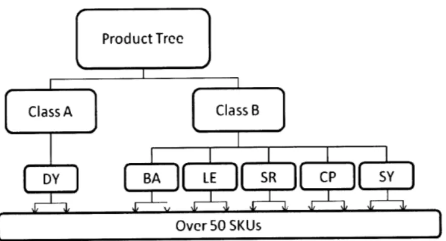
major groups: Class-A and Class-B. Further, in class A there is one product family with 3 products. However, in class B there are 5 product families with a total of 11 products. Moreover, each product has further variants and thus the product portfolio has over 50 stock keeping units (SKU) in total at the finished goods level. To help demonstrate the product relationship, a tree diagram is shown in Figure 1.

Figure 1 Product Tree for PDAP Factory

1.3 Production Process Flow

There are in total 7 production stages for processing SPs in this factory; 4 stages are equipped with

multiple machine lines, each of them manufactures certain types of SPs under the same product family. The remaining 3 stages have only one machine each but those single machines are big and

can handle all the SPs going through the production stage. Due to different process requirements, SPs are not send to all, but a subset of the 7 production stages to complete their own

(14)

Stage 1 Stage 2 Stage 3 Stage 4 age 5 Stage 6 Stage 7

Finished Goods Inventory

Figure 2 Production Process Flow

1.4 Demand Management

1.4.1 Production Planning Process

To begin the production planning process, the National Sales Organization (NSO) in RP Electronics Singapore uses the Advanced Planning Optimization (APO) tool and collaborates with Logistics Management Team (LMT), so as to generate the Monthly Demand Forecast for the coming year by the end of November of the current year. This monthly forecast is then updated each month with a timeframe from then till end of the year. They also provide a weekly rolling orientation values for next 52 weeks with rough estimates for weeks beyond current year. The demand management process can be disintegrated and described below:

1) Development of Monthly Production Schedule (MPS): The Production planner prepares the MPS by the end of third week (on Friday) of current month for the next month (up till end of year) at finished goods level (only) based on the monthly forecast from step 1. The production planner considers only the actual demand and final process capacity while preparing the MPS. The first version of the MPS serves as the basis for a manager who is responsible for developing stock plan as explained in subsequent section. The successive MPS revisions are finalized with assessment from production planner based on his analysis of the comparison between MPS and stock building plan.

(15)

2) Finalization of the monthly demand value: The commercial planner is informed of the capability for one product model, based on which he finalized the monthly demand value for that product model. Some products models have variants, and the commercial planner is allowed to change the demand of particular variant within the demand for the corresponding model, but he is not allowed to change the total demand for that particular product model given in MPS.

3) Weekly Constraint List development: Every Tuesday, the production planner provides a Weekly Constraint List based on his anticipated stock values for the coming week to bind the production planner Weekly Production Schedule (WPS) values.

4) Order placement: The constraints set in step 4 are sent to the commercial planner for planning order placement for next week. The Commercial planner updates order values every week (on Thursday) for next 18 weeks (1 firm while the rest 17 are tentative) at finished goods level considering the constraints provided by the production planner.

5) WPS finalization: Production planner converts the orders sent by the commercial planner in step 5 into firmed WPS for next week and tentative WPS of second next week. Hence the confirmed order for coming week serves as the basis for WPS and Shipment Plan (with 2 days leads to WPS) at finished goods level for production planner.

6) Daily production plan development: The production planner takes into account the first week firmed orders, the first two days order of the following week for assembly plant, and weekly satellite factories requirement from the WPS to develop the daily production plan for different production stages in the factory. He has to do a production leveling based on his own method to match demand with capacity while ensuring on time delivery of shipments. He consider the leveled finished goods requirements, quoted lead times of upstream stages, and individual stage inventory levels to develop a rough daily production plan for all the stages excluding ST. The 6 steps described above are shown in Figure 3.

(16)

Start

Commercial Planner

Monthly Demand Forecast,

Weekly Orders

Monthly& Weekly > Factory

Demand Constraints Planner

Monthly Production Schedule, Weekly Orders

Weekly Production Schedule

End

Figure 3 Production Planning Process

During the high demand season, the production requirements are decoupled from the shipment schedules because the factory builds up stock for the high runners in the low demand season. So the production planner usually tends to run bigger lots of every model to save on changeover times. However, the low runners are not stocked during the low demand season, so they have to be planned following the 6 steps described above.

1.4.2 Semi-Knocked Down (SKD) Parts Demand Management

SKD Manager receives forecast and confirmed orders directly from the satellite factories. The shipments to satellite factories are made on weekly basis and these planned requirements are given to the production planner so that he can plan accordingly. This factory also supplies

(17)

Chapter 2 Problem Statement and Project Objective

This chapter describes the main problems unveiled in the current PDAP manufacturing system, and the objectives of the team project. There are 3 main problems identified in the production system: the first is the demand seasonality, which causes problems in capacity planning; the second problem is their current production control policy that has generated more-than-required intra-stage inventory; the third problem is the desynchronized local production scheduling at each production stage that makes the system erratic. Based on these 3 problems, the project objective becomes to develop an improved production planning and inventory control system for the PDAP factory.

2.1 Problem Statement

2.1.1 Demand Seasonality and Stock Building

PDAP Singapore experiences peak demand starting from the third quarter of each year, i.e. during July to October, when advanced orders are placed by assembly plants and satellite factories in anticipation for the Christmas sale. This demand is higher than the existing capacity of the factory. The low season starts in November, and continues through January to June in the following year. Factory aims to satisfy all demand at the current operating level without extra investment to expand the capacity, as the added capacity can incur extra operating costs in addition to the initial investment. The company tackles the problem by employing a stock building policy that helps the company to utilize its capacity in the low demand season. The extra units produced in advance are kept at the factory and shipped to assembly plant and satellite factories when the factory capacity alone cannot meet the demand.

The stock building plan is of paramount importance as the production requirements are extracted from it rather than the daily shipment requirements. The capacity of the last production stage is examined to determine if the monthly demands, as projected in MPS, can be satisfied with monthly production. Any excess demand is shifted backwards to the earlier months. These adjusted demand values for the last stage become demand for the previous stage and the sequence follows till the first production stage. The production resources are exposed to requirements based on this plan.

(18)

Hence it serves as the input source for us to perform analysis and calculations.

However, this stock building practice only ensures the satisfaction of the demand, without taking account of the inventory costs incurred. The tradeoff between the extent of stocking and the associated inventory cost is not assessed. Furthermore, this scheme's heavy reliance on human intervention makes it vulnerable to mistakes and forecast errors. It should also be noted that this plan is only on aggregate demand level for SP product lines and it would be the job of the production planner to stock high runner variants based on these monthly targets. A more efficient

and accurate way of making a stock building plan may need to be explored.

2.1.2 Production Control

The planning carried out by the production planner serves as the benchmark for production stages during the rest of the week. It is found that this plan was only given to 5 out of the 7 production stages in the factory, namely Stage 1, 2, 5, 6, and 7, the left 2 production stages have to trigger their own production based on the judgment of the supervisor to the upstream work-in-process level, its own stock level and the manufacturing capacity available. Production planner conducts a daily meeting with the production supervisors to follow up on production targets and shipments. This process is shown in Figure 4, where the block horizontal arrows represent the material flow direction, the straight dash line with arrow represents the planning signal sent from production planner to the individual production stages, and the curved dash line depicts the self-planning of other production stages.

The current production control mechanism results in problems such as unnecessarily high intra-stage WIP levels. Moreover, it does not give Production Stage 3 and 4 any plan to guide their production. Such a system leaves the whole production of this stage subjective to human judgments, and results in unreasonable inventory structure and varying inter-stage customer service level. The process involves a great deal of human factor that leads to arguments and confusion during the actual production.

(19)

Figure 4 Current Production Planning

It is evident that current production control mechanism has issues that cannot support the management goal of establishing a Lean production environment. It was worthwhile to investigate what actually goes wrong and causes problems for the planner and supervisors, and eventually results in large inter-stage work-in-process.

2.1.3 Local Production Scheduling and Inventory Control

The machine lines installed in the factory are all shared resources. Each machine line is capable of processing multiple types of SP. The large SP variety with distinct process requirements adds to the complexity of the total manufacturing process flow. Although all machine lines can handle multiple types of SPs, they can be further classified into two groups: One group has machines that is the only machine within the production stage with huge capacity to process all types of SPs, the other group has machines that are equipped with smaller capacity and dedicate to certain types of SPs under a certain SP family.

In daily operation, the machine lines are usually subjected to simultaneous demand of multiple types of SPs needed by either downstream production stages or demand. The simultaneous demands create the puzzles as what to manufacture first and how many should be produced. Under the current manufacturing operation, both delays of production and overproduction are

subject to line supervisor's performance.

In more detail, the line supervisors tend to follow the production plan finalized in the morning meeting and schedule their production relying on their experience. This results in different

(20)

schedules of individual departments. If there is difficulty in executing the plan (e.g. shortage of raw materials or work-in-process from upstream), they tend to keep the lines running on any other available SP work-in-process (WIP) to maximize the machine utilization, even if the downstream lines do not require those SPs and this practice causes over production. Furthermore, uncertain WIP levels and unsynchronized schedules can cause either deviation of downstream stages from their plans and schedules or over production. As all the supervisors adopt this practice, it further causes abnormal day-to-day non-uniformity of the work-in-process levels and the production stage lead times for the released materials.

The careful investigation of all these leads us to the conclusion that this erratic system behavior is the result of desynchronized production planning and inventory control of involved production stages caused by supervisors' subjective judgment. Hence, a new production planning and inventory control system is needed to optimize the inventory levels along the line. This system will also help individual departments set correct production targets within their capacity constraints.

2.2 Project Motivation

The production system at PDAP factory is a complicated system. Although all the machines at each production stage can be considered as multi-part-type machine in some context, they are relatively different for several reasons. The difference stems from the SPs physical flow requirements along the machine lines, which actually merge and split at certain production stages according to the process requirements. In order to study the production system in a more efficient way, the internship team was divided into two groups, each with two students. The two groups focused on distinct production stages of the PDAP production system.

Among all 7 production stages, the project team focused area included the last 5 stages. Stage 5 and 6 are single-machine-line shared by all SPs that need to go through this process. Since it is a chemical coating process, different SPs can be processed together if they share the same coating. This allows Stage 5 supervisor to exploit the opportunity and schedule the production such that changeover time loss is minimum. As already described in the problem statement section, production planning and inventory control is based on supervisor's judgment and thus causes problems like over production and downstream line starvation.

(21)

Stage 4 and 7 are two similar processes and the flow between them can be characterized as direct flow, flow through Stage 5, flow through Stage 5 and 6 based on the SP process requirements. Since Stage 4 and 7 has close production rates, it provides an opportunity to couple their production.

2.3 Project Objectives

The main objective of the project is to develop an improved production planning and inventory control system for the PDAP factory. The specific objectives are:

1. Evaluate the whole production system and propose a suitable inventory control policy. The

policy is to ensure smooth production and material flow through the whole production line and to improve customer service level.

2. Propose an approach to set up daily production targets at each production stage that is consistent with the chosen inventory control policy.

3. Design an appropriate visual management system at the factory for the solutions proposed

above.

4. Implement 1, 2, and 3 to evaluate the performance of the system and make recommendations to the factory.

In this thesis, the four team members contributed together to the calculation of base stock for their responsible production stages, and developed a Kanban system under the designed guidelines. In addition to that, the author had an individual focus on short-term production leveling, his partner Zia Rizvi [1] worked on simulation and capacitated shipment planning. Youqun [2] and Zhongyuan [3] emphasized on demand seasonality analysis and long-term capacity planning.

Author's Focus

(22)

Chapter 3 Literature Review

3.1Manufacturing Systems

3.1.1 Push Production System

A push production system builds up its inventory according to long-term forecasts [4]. This system

is simple to set up and manage. It works well when the demand is steady and predictable, during ramp-up phase, or for predictable seasonal demand [5]. However, due to the innate forecast errors, such a system is prone to product shortages and overproduction when the demand fluctuates. To buffer against such risks, large inventories are typically kept, especially towards the upstream of the production line. The large inventory buffer renders the system highly inflexible in face of uncertainty.

3.1.2 Pull Production System

In essence, a pull production system only produces what the demand asks for, without relying on forecasts to guide its operation. Ideally, production is identical to demand, eliminating the risk of over production. In a pull system, the material flow and information flow travel in opposite directions. There are three typical ways of realizing pull production in a factory: supermarket pull system; sequential pull system; mixed supermarket and sequential pull system [6].

In the supermarket pull system, a safety stock is kept for each product, from which the downstream processes could directly pull. The process upstream of supermarket is only responsible for replenishing whatever is withdrawn from the supermarket. This arrangement enables short production lead-time when demand arrives. The inventories in the supermarket could also be used to help level production. A sequential pull system converts customer orders into a "sequence list" which directs all processes to complete the orders. The production schedule is placed at the first stage of the production line. Then each process works sequentially on the items delivered to it by the previous process. As a result, there is no need for large system inventories. Yet, this may lead to longer production lead-time and requires high system stability to perform well.

(23)

A mixed system of the above two could be applied to reap their distinct advantages. In a mixed system, the supermarket pull system and sequential pull system could operate in parallel on different products.

3.1.3 Push-Pull System

In practice, pure pull system may not always be possible. In some occasions, a combined push-pull system is constructed to exploit the benefits of both. Usually, push is adopted at the back end of the system to cut production lead-time, while the front end is operated by a pull strategy to limit inventory levels.

3.1.4 Customer Service Level

Customer service level is a crucial measure of production system performance. It measures the system's ability to satisfy the demand delivered to the system in a timely manner. Although its actual definition may vary, two definitions are commonly used [7]:

Type I: Probability of stock out when there is an order. Type II (fill rate): Percentage of demand met from inventory.

3.2 Inventory Control Policies

To initiate Lean manufacturing in this factory, one of the most important topics is the implementation of a right inventory control policy. There are lots of literatures talking about inventory control policies. MIT lecture material of course 15.763 discusses two inventory control policies for stochastic demand in general, one is Q-R policy and the other is Base Stock policy.

3.2.1 Q-R Policy

The main concept of Q-R policy is to set a reorder point and a reorder quantity. Once the inventory level hits the reorder point, a fixed reorder quantity will be released to the factory floor, and the inventory level is under continuous review. This policy is suitable for dedicated high volume production line. Basic equations and parameters for this policy are shown below.

(24)

1) Reorder Point R:

R = Expected lead-time demand + safety stock

R =/ L+zaoL (3-1)

2) Average inventory level throughout the time window E[I]: E[I]= cycle stock + safety stock

E[I] E[I-] + E[I+] = + zor- (3-2)

2 2

*

Q: re-order quantity * pt: demand rate

* r: review period in days

* z: safety factor

* 6: standard deviation of demand * L: lead time for replenishment

3.2.2 Base Stock Policy

The main concept of this policy is to set a base stock level and a review period. Inventory level will be reviewed every fixed review period. If it is lower than the predetermined base stock level, production order will be released to the factory floor to replenish the inventory level to the base stock level. This policy is suitable for shared resource line with multiple products. Basic equations and parameters are shown below.

Base stock B,

B = u(r + L) + zc -r L (3-3)

Average inventory level throughout the time window E[I], E[I]= cycle stock + safety stock

E[I(r + L-)]+ E[I(r + L)] + zr (3-4)

E[I]= = -+ Za (3-4)

2 2

r: fixed review period

The parameters used here are the same as in Q-R policy

(25)

The Q-R policy is suitable for dedicated resources whereas the production system studied in this thesis has production resources with heavy sharing by multiple resources in downstream. This can cause simultaneous replenishment signals and eventually prioritization will affect the performance of the policy. Base stock policy may be a better choice for this case where replenishment of individual model inventories can be carried out in different review periods but there are also some limitations of the same.

Conventional base stock policy assumes that a production stage can be operated under a fixed and deterministic lead-time. This can be a good approximation for single product processed on such a resource. Since the production lead times are predetermined and fixed, there are no interactions between the production decisions and inventory levels of different products processed on the shared resource. It implies that the base stock planning is carried out in isolation for each product but setting up individual review periods would still be subjective as there is no systematic

approach that considers the resource capacity constraints.

Moreover, fixing a lead-time of a production resource implies that it is completely flexible in context of its ability to change production rate but it doesn't explicitly take into account the trade-off between flexibility and base stock levels.

3.3 A New Base Stock Policy for Multi-Part-Type Line

Base stock model proposed by Prof. Stephen Graves in "Safety stock in manufacturing systems", 1988, dealt the limitations of conventional base stocky policy for shared resource. This model takes the capacity constraint of the production line into account, and works well in smoothing daily production of a multi-item machine using a linear production rule and determines each model's individual inventory level (B,). Some of the key calculations and parameters of the model are listed as follows:

a) Proposed lead time by considering machine flexibility to expedite production and demand variations

(k2o2 + 2)

n = (3-5)

(26)

k = parameter that is associated with customer service level 6 = standard deviation of weekly demand

X = excess capacity

b) Daily leveled production

W D (n 1)P

-P 1 -+ (3-6)

n n n

t: time period index

P: daily production quantity D: daily demand quantity W: WIP at the production stage

c) Individual model (s) 'i' raw material released exactly equal to demand on day 't'

R,,, = Di,, (3-7)

R: material release quantity

d) Base stock for individual model(s)

B, = E[W,,] + E[I,,,]= ni + k[no' 42n-1] (3-8)

[ti: average demand for item i

3.4 Visual Management

Visual management uses visually stimulating signals, objects and easy-to-understand symbols to creat and information-rich environment. In simple terms, visual management uses signs, lights, notice board, bright or contrasting painted equipment to display information and catch people's attention, so as to enhance the communication of important information or messages in the working environment [8].

In Lean manufacturing, the goal of visual management is simply generating meaningful signals, and facilitate people in factory to access information about what their tasks quickly and accurately, especially for those who do not hold any knowledge of the logic behind the High Tech solutions

(27)

are not necessary to bring about visual management, the rule is "the simpler the better", simple tools such as photos, painted symbols, bold print and informative colors are usually more robust.

As Lean manufacturing system is to be easily understood and continuously monitored, an appropriate associated visual management system is really critical to the successes of all Lean operations. Nowadays the most developed and widely used visual management tool in factories is called the Kanban system, which has all the features noticed above.

(28)

Chapter 4 Methodology

4.1Project Flow

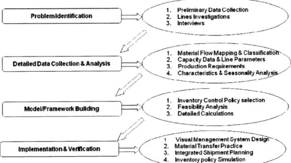
As shown in Figure 6, a project roadmap shows the sequence of major project stages and specific activities involved. Rectangles represent project stages and ovals represent detailed activities of the corresponding project stages. The arrows represent the sequence.

Problemldentification

Detailed Data Collection & Analys

Model/Framework Building

Implementation&Verffication

1. Preliminary Data Collection

2. Lines Investigations "

3. Interviews

1. Material Flow Mapping & Classificatto- ,

Is C 2. Capacity Data & Line Parameters 3. Production Requirements

4. Characteristics & Seasonality Analysis~

1. Inventcry Control Policy selection

2. Feasibility Analysis )

3. Detailed Calculations

1 Visual Management System Design

2. MaterialTransfer Practice

3. Integrated Shipment Planning 4. Inventory policy Simulation

Figure 6 Project Roadmap

4.2 Problem Identification

The project started with the problem identification stage. The author was initially given briefing on what the management was aiming to achieve in the future; then the project team focused in depth on the production floor issues that were the biggest potential obstacles. Interviews were conducted with the production planner and supervisors to understand the production process of the SP assemblies at PDAP, and to identify the issues that these people were facing. The inventory profiles from history were shown; real data was collected for later comparison. The major issues had already been discussed in Chapter 2.

(29)

4.3 Data Collection and Analysis

As part of the preliminary research, the data relevant to the project was collected and sorted into two categories: structural data and quantitative data. Structural data included the material flow mapping, product categories, factory layout, and the value stream map of the factory. Quantitative data included line performance data, historical demand data, demand forecast data and inventory data.

4.3.1 Source of Data

In order to understand the general demand characteristics throughout the year, daily shipment data for 2008 were obtained from the production planner for analysis. The daily shipment data detailed the shipment volumes of all SKUs to the customer. Hence, these data were treated as the best source of the historical demand.

The demand forecast and stock building plan files for 2009 were also obtained from the production planner. The forecast provided the predicted monthly demand from customers, and the stock building plan was used to shift some demand to be fulfilled earlier with consideration of capacity constraints. The stock building plan file was used as the input for the inventory control policy calculation, which was the most accurate data currently used to plan production.

4.3.2 Planned Production Seasonality Analysis

Demand driven production is one important feature of Lean Production to eliminate waste and increase profit. In PDAP factory, the planned production targets specified in the stock building planned is used as the actual demand from the manufacturing perspective of view. Hence, to properly select the inventory control policy and calculate the respective inventory levels, the seasonality analysis to the stock building planned was needed.

As mentioned in Section 1.2, there are two product categories in this factory: Class A and Class B products. Class A is about 30% of the total demand, and Class B is about 70% of the total demand. Because Class B products were mostly sold in America and Europe, holidays in these regions such as Christmas had heavy impacts on the demand of Class B product. This formed the seasonality

(30)

demand pattern for Class B product. However, for Class A product, since they were sold mostly to where the holiday effect was not so influential, the demand for Class A products is more consistent throughout the year. In the end, for simplicity, the seasonality analysis considers Class A and Class B demand together.

The task here is to determine the seasonality of total demand volume throughout a year, verify and improve the current pattern that the factory is now following in production. To achieve this goal, the planned production values are retrieved from the 2009 stock building plan, monthly production targets are obtained. Then, several potential groupings of seasons are proposed and analyzed by ANOVA, the distinct seasons are therefore chosen based on the F-value and P-value from ANOVA for the grouping that provides the highest F-value and lowest P-value. See Figure 7.

Demand Stock

Forecast Building_Plan

Seasons Grouping 1 Seasons Grouping 2 Seasons Grouping 3 *0 0

z

₁

Selected

4

ANOVA =4 Seasons Grouping Seasons Grouping n

Figure 7 Procedures of Seasonality Analysis

4.3.3 Selection of High Runners & Obtain Daily Demand Pattern

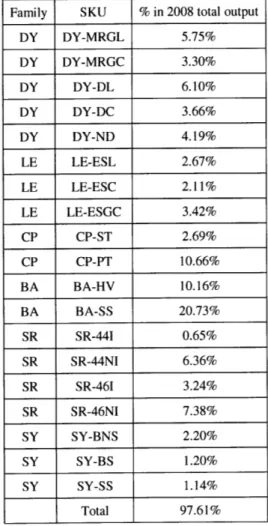
The total demand is formed by gathering individual demand from over 50 SKUs produced in this factory. However, not every SKU receives constant level of orders. The majority of the total demand comes from a group of popular SKUs, which are called the high runners. To optimize the inventory structure, the new base stock policy will only be applied to the high runners. Constant inventory will be kept only for them at each of the production stages involved to facilitate the pull manufacturing. The production for the non-popular SKUs will follow the push-based planning, and this aspect is not the focus in the thesis.

(31)

The selection of high runners was primarily based on the historical demand records. Both the shipment frequency and quantity were considered. The production planner also made suggestions for selecting several new SKUs as high runners, which were recently released to the market, and no long-term shipment record was available.

Because of the need to obtain the daily demand and standard deviation from the 2009 stock building plan, some data processing is required. In the stock building plan, the demand volume is specified only on a weekly basis. Moreover, instead of individual SKU, only the aggregated demand for each product family or a group of similar SKUs was available. So first of all, the aggregated daily demand and its standard deviation can be obtained as follow:

d= L d = 0 (4-1)

77

Further data processing was needed to dig out the demand pattern for each individual SKU considered as high runner. A reasonable assumption is made here, that the demand for all SKUs within the same product family will share identical coefficient of variance (C.V.). Also, it is assumed that their contribution to the total demand volume is assumed to be the same as the 2008 demand records with approval from the production planner. Once the weekly demand is obtained for individual SKU, the daily demand pattern is calculated by the following formula:

1) Let n be the number of SKUs within a certain family, i is the index of different SKU under the same product family.

(4-2) 2) Assume all SKUs share the same individual C.V., then the C.V. can be calculated as

follows:

0 2 (CV xl,d )2 + (CV XU2,d)2 +...+(CV X/13,d) 2 (4-3)

2

CV = d (4-4)

3) With C.V. obtained for individual SKU and the mean, the demand standard deviation of individual SKU can be determined as:

(32)

Figure 8 shows the procedures:

2008

Shipment

Ddtd Aggregated DailyMean

' d ' Selection of Weekly _&_{STD for}

High Mean& _Individual

Runners STD SKU

Production Planner

Figure 8 High Runner Selection & Daily Demand Pattern for Individual SKU

4.3.4 Line Data & Performance Measures

Various important process parameters for each production stage were obtained from the factory. Among them, the most important one was the effective capacity from each machine line. With the capacity file given by the production planner, weekly effective capacity were shown, thus the daily capacity were obtained with simply calculation.

In addition, process lead times and cycle time were collected for several SKUs. Other critical production line performance measures, such as the inventory levels at each production stage (WIP and FGS) were obtained. The inventory levels at each production stage were tracked using data maintained in SAP system. Data were extracted from the system and compiled for specific production stages. Inventory holding costs and unit costs of components at all the stages were provided by the factory.

4.4 Production Leveling

As stated in Section 1.4.1, the daily production plan was finalized by the production planner based on the locked demand of next week plus the following two days' orientation. The weekly satellite factory requirement (SKD) was also considered. With the consolidated demand file on hand, the production planner then leveled the production from his own experience so that he could match demand with available capacity while ensuring on time delivery of shipments. As the production

(33)

plan will be issued to 4 production stages. The quoted lead times of upstream stage, and individual stage inventory levels are also considered and therefore add complexity into the planning.

Leveled Production Targets Original Demand

Production Leveling

Figure 9 Objectives of Production Leveling

With the goal of improving the production planning process within this factory, the above stated operations can be simplified into setting the production targets only at the end production stage for each SKU. With the requirement of fulfilling demand from the customer side and the goal of smoothing daily production, an optimization tool for production leveling is developed. In the following context, three different methods are proposed and compared, the first two methods are generic, and the last one is an improved one based on the first two methods.

4.4.1 Heuristic Method

The Heuristic Method is a manual method developed to leveling the daily production targets. The leveling period is chosen to be 7 days to reflect the real scenario, the operation procedures are shown in sequence below

1) Leveling input & output:

Input Demand: D, i= 1, 2, 3 ...., 7

Production Target: P, i=l, 2, 3 .... 7

2) Production constraints:

(i) The accumulated production must always be equal to or higher than the demand

-P 2 D i=1,2,3,. ..., 6 (4-6)

(ii) The total production quantity at the end of the leveling period must be equal to the total demand to avoid overproduction.

(34)

-P = -D i= 7 (4-7)

3) Objective:

The leveling effect will be evaluated by the coefficient of variance of P, i=l, 2, 3 ... 7

Minimize: C.V.(P,) i=l, 2, 3, ..., 7

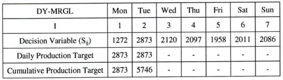
4) Calculation:

(i) To determine P,, a decision variable S, (i,j=O, 1, 2, ..., 7 i<j) is introduced. S, is a calculated value. It is obtained by the formula shown below:

SI (4-8)

j-i

With Sl, the daily production target P, can be determined in sequence, starting from Pi (ii) To getP,, So, (j=0, 1, 2,..., 7) is calculated to look for its maximum value and the

respective j. Once jmax is obtained, let ni=j-0=j. Then P1 is calculated by the following formula. If n>l1, then P = P2... = Pn, and the calculation can jump to day nl+l.

Pl = ...- = PD (4-9)

'

j-0

n,

(iii) Starting from day nl, again we need to calculate and compare the S,, for another round, the maximum S,,j shall be obtained.

S j= (4-10)

j = n, +1, ... , 8

With maximum S,, , denote the currentj by n2, then a new set of production target will be obtained:

P,+1 = pn.. = 0 = i (4-11)

2+ -n 1 n2 2 -n1

(iv) Repeat the calculation until P, is obtained

(35)

Excel Solver is a build-in optimization tool in Microsoft Excel. With the same objective and constraints specified in the Heuristic Method, the leveling process and requires less effort to operate in the Excel Solver. By properly setting the objective function, design variable and constraints, the optimized result can be obtained quickly. To explain the details, the leveling procedure is decomposed into the following 6 steps, also shown in Figure 10:

1) Input the daily original demand data

2) Calculate the accumulative demand for each day

3) Set the initial values of production quantity for each day and appoint them as variable cell. The initial value can be the same as the original daily demand.

4) Set production constraints

5) Run Excel Solver

6) Obtained the result and verify it by plotting the demand and the leveled production for each day within the leveling period.

Input the daily demand for the whole leveling period Calculate accumulative demand for each day in the leveling period

Input initial value of leveled production targets

Set up production constraints into the Solver

Run Solver

Obtained level production targets

for each day &verification

(36)

4.4.3 Improved Excel Solver Method

On each Thursday, the production planner receives locked (confirmed) demand for the next Monday to Sunday. By considering the two days' shipment lead time, the previous leveled production targets are able to be modified, so as to prepare for the possible demand surge at the beginning of the next week. In addition, the two days' demand orientation followed by the locked demand is included into the leveling period. The leveling process will still be done by Excel Solver, and it is called the Improved Excel Solver Method

Finished Goods

Day 1 Day 2

S< Destn ation

Day3 Figure 11 Shipment Lead Time

The main operation procedures for the optimized Excel Solver Method will still remain the same as the previously introduced Excel Solver Method. However, since the leveling periods are now overlapped by 3 days, and the shipment lead time takes only two days, one modification must be made to the demand input, so that overproduction can be avoided. The new leveling periods is

demonstrated in Figure 12.

Locked Demand Thu Fri Sat

--- --- -- ->Th u

Sun Mon Tue Wed Thu Fri Sat Sun I

A A Demand Time Line

I I

Sat Sun I Mon Tue Wed Thu Fri

Oricntation

Mon Tue

Sat Sun I Mon Tue

Manufacturing Time Line Figure 12 Optimized Excel Solver Method

As now the leveling periods are overlapped by three days, the remaining 7 days production targets in the previous leveled period will not change. But in most cases, the first 7 days total production volume is higher than the demand volume. If the excess is not subtracted from the demand in the new leveling periods, which is overlapped with the previous one, over production will happen. The subtraction will first be done from the first day of the new leveling periods, until all the overproduced quantities are consumed by the demand in the new leveling period. Details will be shown in the result section.

I

(37)

4.5 New Base Stock Policy

4.5.1 Model Building

The new base stock policy was developed in 1987 at MIT by Professor Stephen C. Graves. This policy specifies new production control rules and calculation of inventory levels for each product manufactured on the same machine line. This policy is able to model multiple machine lines and can be extended to a multi-stage manufacturing system. However, for demonstration purpose, one production stage that processes multiple SKUs is chosen here to explain how the new policy

works. Below is a list of important parameters used for the calculation:

D: Demand

R: Release of raw material P: Manufacturing quantity B: Base stock level C: Line capacity

W: Intra-stage inventory I: Inter-stage inventory t: Time period index

* i: Individual SKU index * n: Planned lead-time

*

X: Excess capacity that is normally available at the production stage

* [t: average demand

* 6: standard deviation of demand * k: Safety Factor

It and Wt are aggregate inter-stage and aggregate intra-stage inventories at time period t, they can also be interpreted as finished goods inventory and raw material inventory at a certain production stage. Pt and Rt are manufacturing target and quantity of raw material release at time t. The random variables It, Wt, Pt, Rt are aggregated entities while litit, t, Pt, Rit are entities for individual model. For example: It=Int, where lit is the inter-stage inventory for product I at the start of time period t

The balance equations for aggregated entities are:

(4-12) (4-13)

w, = W,_l +R, - -1

(38)

The release rule is: R, = D, (4-14)

These equations can be easily extended to individual entities, namely:

W t = Wi,t_ + R,, - P,,t-1 (4-15)

Ii, = li.-1 + Pi,-1 - Di, (4-16)

The release rule becomes: R, = D (4-17)

The other two important parameters are X and n, both of them obtained by calculation: X= Line Capacity -Aggregated Average Demand

(k2 2 2 )

(4-18)

n = (4-18)

2Z2

With the mathematics behind the theory, x should be less than or equal to k*6, otherwise n is equal to l.

With X and n determined at each production line, the control rules for individual model i are given by:

R,' = D,,, (4-19)

W,,

pt = (4-20)

n

And the expected inventory values for individual SKU i are given by:

Bi = E[W,,] + E[I,,,] = np + k[noiJn-I ] (4-21)

Hence, for the later calculation, the E[Wit] and E[lit] will be obtained for every selected SKUs at each production stage with consideration of reasonable grouping. And the floor production will execute according to:

P = W" W (4-22)

(39)

With Equation 4-22, the daily manufacturing quantity is determined, which usually differs from the daily production target. Moreover, since the n and Wit at each production stages are usually different, for the same SKU, the daily manufacturing quantity will be different.

4.5.2 Preliminary Calculation & Modified Results

Based on the demand information for high runners and the calculation specified in Section 4.5.1, the base stock level for each high runner at every involved production stage can be determined accordingly. However, this result only contains the theoretical value and ignores all implementation constraints. Modifications are made to comply with these constraints, the details

are discusses later.

4.5.3 Kanban Implementation & Other Implementation Issues

The most important part of the project work verification lies in the implementation and modification stage. From the management requirement, a Kanban system will be set up throughout the factory to operate under the new base stock policy, many implementation issues are raised by the constraints not considered is the new base stock policy but in the factory.

Kanban card design

To set up a Kanban system in PDAP factory, the design of the Kanban card is important. Since this factory has previous experience on designing and using Kanban cards for some special operation, the author choose to adopt their current design and made necessary modifications. The contents on the card are listed below:

(40)

1) Card ID number 4) Represented quantity 2) Name of the model 5) Production Stage 3) Part transit number (12NC)

Kanban quantity

Being part of the information shown on the card, the represented quantity of each Kanban card (Kanban Quantity) is critical to the designed pull system and must be carefully determined. To choose the right Kanban Quantity, investigations have been done on the containers used for material transfer among different production stages. Suggestions are made to modify the size of various containers, so as to synchronize the sizes. As a universal quantity represented by a card would greatly simplify the operation of the system, the size of containers is modified to either an factor or multiples of standard pallet size for shipment. The shipment size is 600 or 480 according to different SKUs, thus 600 and 480 will be the quantity represented by each Kanban card in all production stages involved (Stage 4, 5, 6 and 7).

Determine number of cards required

With the quantity represented by each card determined and the calculated base stock level, the total quantity of cards can be determined. The results were stated in Section 5.6.2.

Kanban operation procedure

The new base stock policy specified strict control rules and operation procedures in withdrawing raw material, setting daily manufacturing quantity, and finished goods shipment. In the Kanban system designed to operate according to the new base stock policy, all material transfer will be guided purely by the movement of cards. The number of cards shown on the Kanban board will

(41)

be used to monitor the real time inventory levels and the manufacturing activities. The details are stated in Section 0.

Modifications to Production Leveling

After leveling by Excel Solver, the output values will not be multiples of 480 or 600. Thus to assign daily production targets correctly by moving the Kanban cards, the numbers need to be modified. An extra step is needed after leveling to round up the daily production targets to multiples of 480 or 600. The details are shown below:

1) Modify every day production targets to multiples of 480 or 600

2) Add constraint so that the accumulative value after modification is more than or equal to the accumulative production targets provided by Excel Solver

It is found out that after this modification, the accumulative production targets will be slightly more than the demand quantity. However, after consulting the production planner, this concern is not necessary, as the customer will be able to adjust their order slightly in the next week if they receive more finished goods in the current week.

4.6 Line Coupling

SKUs belong to the CP and SR families pass through production stage 4 and 7 as a direct flow. From the original base stock calculation, W and I inventory will be set up separately for each SKU at both stage 4 and 7, so are the CP and SR SPs. However, with an interesting finding that the capacity of machine lines at these two stages are very close or even equal to each other, they can be virtually linked together by a specially designed coupling stock. By doing so, the I inventory