Sovereign Debt Risk in Emerging Countries: Does Inflation Targeting Adoption Make Any Difference?

HAL Id: halshs-01128239

https://halshs.archives-ouvertes.fr/halshs-01128239v2

Preprint submitted on 25 Mar 2015

HAL is a multi-disciplinary open access archive for the deposit and dissemination of sci-entific research documents, whether they are pub-lished or not. The documents may come from teaching and research institutions in France or abroad, or from public or private research centers.

L’archive ouverte pluridisciplinaire HAL, est destinée au dépôt et à la diffusion de documents scientifiques de niveau recherche, publiés ou non, émanant des établissements d’enseignement et de recherche français ou étrangers, des laboratoires publics ou privés.

Weneyam Hippolyte Balima, Jean-Louis Combes, Alexandru Minea

To cite this version:

Weneyam Hippolyte Balima, Jean-Louis Combes, Alexandru Minea. Sovereign Debt Risk in Emerging Countries: Does Inflation Targeting Adoption Make Any Difference?. 2015. �halshs-01128239v2�

C E N T R E D'E T U D E S E T D E R E C H E R C H E S S U R L E D E V E L O P P E M E N T I N T E R N A T I O N A L

SERIE ETUDES ET DOCUMENTS

Sovereign Debt Risk in Emerging Countries:

Does Inflation Targeting Adoption Make Any Difference?

Wenéyam Hippolyte BALIMA

Jean-Louis COMBES

Alexandru MINEA

Etudes et Documents n° 4

February 2015

To cite this document:

Balima W.H., Combes J.L., Minea A. (2015) “Sovereign Debt Risk in Emerging Countries: Does Inflation Targeting Adoption Make Any Difference?” Etudes et Documents, n° 4, CERDI.

http://cerdi.org/production/show/id/1658/type_production_id/1 CERDI

65 BD. F. MITTERRAND

63000 CLERMONT FERRAND – FRANCE TEL.+33473177400

FAX +33473177428

The authors

Wenéyam Hippolyte Balima PhD Candidate

Clermont Université, Université d'Auvergne, CNRS, UMR 6587, CERDI, F-63009 Clermont Fd Email: weneyam_hippolyte.balima@udamail.fr

Jean-Louis Combes Professor

Clermont Université, Université d'Auvergne, CNRS, UMR 6587, CERDI, F-63009 Clermont Fd Email: j-louis.combes@udamail.fr

Alexandru Minea Professor

Clermont Université, Université d'Auvergne, CNRS, UMR 6587, CERDI, F-63009 Clermont Fd Email: alexandru.minea@udamail.fr

Corresponding author: Alexandru MINEA

Etudes et Documents are available online at: http://www.cerdi.org/ed

Director of Publication: Vianney Dequiedt Editor: Catherine Araujo Bonjean

Publisher: Chantal Brige-Ukpong ISSN: 2114 - 7957

Disclaimer:

Etudes et Documents is a working papers series. Working Papers are not refereed, they constitute research in

progress. Responsibility for the contents and opinions expressed in the working papers rests solely with the authors. Comments and suggestions are welcome and should be addressed to the authors.

Abstract

Based on a sample of 38 emerging countries, we find that inflation targeting (IT) adoption improves sovereign debt risk. However, we show that IT adoption effectiveness is sensitive to several

structural characteristics, such as the phase of the business cycle, the fiscal stance, and the level of development. In addition, the measure of the risk, namely ratings (rating agencies) or bond yield spreads (markets), as well as the form of IT (full-fledged or partial) is equally crucial for the effects of IT adoption on sovereign debt risk. Thus, our paper provides valuable insights for IT implementation as a device for improving emerging market economies’ access to international financial markets for financing long-term investment projects and supporting potential economic growth.

Key words: Inflation targeting; Sovereign debt ratings; Government bond yield spreads, Emerging markets; Propensity scores matching

I. Introduction

The recent crisis engendered major macroeconomic imbalances, such as large unemployment, low economic growth, rapid expansion of government debts, and fiscal and current account deficits. This resulted in a worsening of access conditions to financial markets, and particularly in a sizeable increase of sovereign debt risk. According to Csonto & Ivaschenko (2013), the government borrowing cost of emerging markets, measured by the JP Morgan EMBI (Emerging Market Bond Index), quadrupled from 200 (beginning of 2007) to more than 800 basis points (end of 2009). Consequently, the debate on the determinants of sovereign risk is currently into the spotlight.

There exists an important literature on the determinants of sovereign risk, especially in emerging countries. Risk is generally measured by (i) government debt ratings from notation agencies, (ii) yield spreads with respect to a country’s sovereign bonds assumed as risk-free, or (iii) Credit Default Swaps (CDS) spreads. In one of the first contribution using measure (i), Cantor & Packer (1996) employ Moody’s and Standard and Poor’s ratings for 49 countries, and find that higher ratings are due to higher income per capita, rapid GDP growth, low inflation, low external debt, high level of economic development, and the absence of default history. Capitalizing on these findings, subsequent studies emphasized additional determinants of ratings, such as exchange reserves or the current account balance (Bissoondoyal-Bheenick, 2005; Afonso et al., 2011; Ratha et al., 2011), the fiscal balance, trade openness or institutions (Bario & Packer, 2004; Depken et al., 2007), the political business cycle (Block & Vaaler, 2004), or fiscal transparency (Hameed, 2005). Moreover, the major determinants of (ii) government bond yields are domestic macroeconomic fundamentals (Edwards, 1986; Cline, 1995; Cline & Barnes, 1997; Borio & Packer, 2004; Berganza et al., 2004; Baldacci & Kumar, 2010; Arezki & Brückner, 2012; Hilscher & Nosbusch, 2010; Baldacci et al., 2011; Hatchondo et al., 2012; Comelli, 2012; Aizenman & Jinjarak, 2012; Eichler, 2014; Costantini et al., 2014) and global conditions in financial markets and international factors (Arora & Cerisola, 2001; Sy, 2002; Bellas et al., 2010; Jaramillo & Tejada, 2011; Arslanalp & Poghosyan, 2014), including GDP growth, public debt, foreign exchange reserves, inflation rate, crisis episodes, and the FED interest rate. Lastly, a recent literature using (iii) CDS spreads attributes high market default risks to weak macroeconomic fundamentals and global market factors (Pan & Singleton, 2008; Zhang, 2008; Aizenman et al., 2013; Longstaff et al., 2011).

In this paper, we contribute to the literature on the determinants of sovereign debt risk by analyzing how rating agencies and bondholders perceive the sovereign risk of inflation

targeting (IT) countries, compared to countries under money or exchange rate targeting. Indeed, simple stylized facts reported in Appendix 1 show that (i) the majority of the twelve emerging countries that adopted IT experienced a substantial improvement in their credit rating after having adopted IT; and (ii) following IT adoption, bond yield spreads decreased in three-fourth of emerging IT countries. In complement to these illustrations, several theoretical arguments support the idea that IT countries could be treated differently by rating agencies and financial markets in terms of sovereign debt risk.

First, previous studies found that, due to the limits it imposes on seigniorage revenues, IT adoption improves fiscal discipline (Minea & Tapsoba, 2014), by reforming the tax system or rationalizing public expenditure1 (Rose, 2007; Freedman & Ötker-Robe, 2009; Lucotte, 2012). Such efforts constitute significant progress towards achieving compliance with the government intertemporal budget constraint. In turn, the improvement of fiscal discipline may increase the willingness and the ability of government to repay the debt and its burden on time. As shown by Heylen et al. (2013), a fiscal consolidation contributes significantly to debt reduction in the long-run. We should therefore expect a reduction in sovereign debt risk following IT adoption.

Second, several studies highlighted that monetary policy can have an indirect effect on fiscal effort through inflation eroding the real value of taxes (the Keynes-Oliveira-Tanzi effect, Tanzi, 1992). In addition, many authors showed that IT is more effective than other monetary regimes in reducing the level and volatility of inflation, especially in emerging countries (Vega & Winkelried, 2005; Gonçalves & Salles, 2008; Lin & Ye, 2009, 2012). Thus, IT could mitigate the Keynes-Oliveira-Tanzi effect, and limit the uncertainty on tax revenues. This may ultimately increase government solvency, thereby reducing sovereign debt risk.

Third, the mere perennity of IT is crucially related to central bank independence and transparency, which affect the credibility of monetary authorities. Moreover, the credibility of fiscal and monetary authorities is a key discriminating factor to access international capital markets, as illustrated by the recent debt crisis experienced by several Eurozone countries. Consequently, IT adoption can send a strong signal for macroeconomic reforms, with positive consequences on government debt risk.

Finally, we can add two additional substantial motives to these arguments supporting a potential favorable effect of IT adoption on sovereign debt risk. On the one hand, according to

1 _{For example, in Turkey, the reforms of the statutes of the central bank engendered by the IT implementation in}

January 2006 (under the auspices of the IMF and in close coordination with the fiscal authorities), were accompanied by fiscal policy improvements, in the form of the announcement of annual primary surplus targets.

the “Fisher effect” (coined by Irving Fisher, 1930), an increase in expected inflation erodes the real value of the return on government bonds, thus decreasing (and increasing) the demand (supply) for bonds, and further increasing interest rates on bonds. Through involving low inflation rates, IT adoption cools down inflation expectations, and therefore reduces bonds yields. On the other hand, according to the theory of purchasing power parity (PPP), a rise in inflation generating the depreciation of the domestic currency negatively affects investors’ expectations about a country’s ability to repay its public foreign currency debt, and thus can increase bond yield spreads. Given its performances in reducing inflation, IT adopting could affect rating agencies and investors’ views on sovereign debt risk.

Despite a large literature evaluating the effects of IT on several macroeconomic variables,2 no study has yet estimated the relationship between IT adoption and sovereign debt risk, with the notable exception of Fouejieu & Roger (2013). In this paper, we develop their analysis on several grounds. First, in addition to government bond yield spreads, we use a second measure of sovereign debt risk, namely government debt ratings from notation agencies.3 This allows distinguishing among sovereign debt risk from the perspective of rating agencies and investors, respectively. Indeed, while bond yield plays an important role in determining the cost of capital, debt ratings play a central role in determining both the cost and the capital flows across countries. Moreover, not only the direction of causality between ratings and spreads is subject to debate,4 but some studies highlight that ratings have little market impact or fail to predict crisis episodes (Reinhart, 2002; IMF, 2010). Finally, differences in risk’s perception by credit agencies and markets are supported by a simple illustrative comparison. Despite sharing the same rating grade in 2011-12 (“BBB”, according to S&P), Brazil and Bulgaria displayed significantly different spreads during the same period. Therefore, it is vital to go beyond a unique measure of sovereign debt risk, in order to appropriately assess the consequences of IT adoption.

2 _{For example, many studies, including e.g. Levin, Natalucci & Piger (2004), Petursson (2005), Vega &}

Winkelried (2005), Batini & Laxton (2007), Mishkin & Schmidt-Hebbel (2007), Rose (2007), Gonçalves & Salles (2008), Lin & Ye (2007, 2009, 2012, 2013), Frappa & Mésonnier (2010), Lin (2010), Miles (2007), Abo-Zaid & Tuzemen (2012), Bleich et al., 2012, Ftiti & Hichri, 2014, Minea & Tapsoba (2014), defend the merits of IT adoption for a wide range of monetary or real goals. Nevertheless, other studies emphasize negative (Brito & Bystedt, 2010) or inconclusive (Ball & Sheridan, 2005; Ball, 2010) effects of IT adoption.

3 _{The only reason for abstracting of CDS as a third measure of sovereign debt risk is that the largest majority of}

countries in our sample adopted IT previous to the publication of CDS data (for example, Bloomberg or Reuters report CDS only starting 2004).

4 _{For example, Hartelius et al. (2008), Jaramillo & Tejada (2011), and Sy (2002) find that rating changes}

significantly impact yield spreads, contrary to Gonzalez-Rozada & Yeyati (2008) who conclude that rating changes respond to, rather than influence, spreads.

Second, IT adoption is subject to a self-selection bias. Following the literature on the effects of IT adoption, we consider IT as a natural experiment and draw upon recently-used propensity scores matching (PSM) methods (Vega & Winkelried, 2005; Lin & Ye, 2007, 2009, 2012, 2013; Lin, 2010). In particular, PSM have the merit of properly identifying the control group through a list of well-identified observed variables.5

Third, compared to Foujieu & Roger (2013), we made the choice of focusing our analysis exclusively on emerging countries, for the following reasons. To begin with, emerging countries are particularly concerned with the issue of sovereign debt risk, because of the large amount of capitals they must raise to further finance their economic development, and also given the large and rapidly expanding size of sovereign debt markets. Furthermore, emerging markets generally display a large variation in the risk of sovereign insolvency, and are among the high-yield borrowers in the world, so the question of the drivers of sovereign risk is a crucial policy issue. Next, since previous studies emphasized notably different effects of IT adoption in developing and developed countries (for example, in terms of fiscal discipline, see Minea & Tapsoba, 2014), it is more appropriate to perform estimations on the more homogenous sample of emerging countries. Last, we significantly enlarge the sample of emerging countries, from 18 in Foujieu & Roger (2013) to 38; (more than) doubling the number of countries is particular important for the robustness of our results, given the use of the PSM technique.

Fourth, we extensively discuss the potential heterogeneity of the effect of IT adoption on both measures of sovereign debt risk, conditional upon a wide set of variables, including the phase of the business cycle, the fiscal stance, and the level of economic development.

Finally, we analyze the impact of IT adoption on bond yield variability. Indeed, given their still fragile integration into international capital markets, emerging countries have historically been subject to high financial stress, often resulting in a sudden massive capital withdrawal and high variability of government borrowing costs.6 As a result, policymakers are concerned not only by the level, but also by the variability of the borrowing cost. By reducing policy uncertainly, IT adoption could better anchor investors’ expectations, thereby reducing the variability of the spreads.

5 _{The choice of this method prevents us from specifying a certain autocorrelation structure in the error term,}

needed to identify lagged variables as valid instruments, as this is the case with the GMM method used by Foujieu & Roger (2013). In addition, we deal with a common critique of PSM methods by controlling for the potential effect of unobservables through submitting our results to such robustness tests.

6 _{For instance, during 1998-2002 Argentina’s depression, the government borrowing cost increased dramatically}

from 476 (December 1997) to 1982 basis points (September 1998). At the end of 2002, Argentina borrowing cost was thirteen times larger than its level in December 1997.

Our results are the following. We find that IT adoption significantly increases sovereign debt ratings and decreases government bond yield spreads in emerging markets. The magnitude of this favorable effect is economically meaningful, namely between 2 and 4.5 pp for spreads, and an additional 2 rating grades. In this latter case, IT adoption can move emerging countries to investment grade status that can considerably increase and diversify their investors’ portfolio. The robustness of these results is supported by several post-estimation tests, and by a wide set of specifications, such as abstracting of “dollarized” countries, hyperinflation episodes, or oil exporters, accounting for additional covariates, and drawing upon alternative specifications for computing propensity scores.

In addition, we explore the heterogeneity of our findings by disaggregating the sample according to several structural characteristics, including the level of economic development, the phase of the business cycle, and the fiscal stance. Regarding sovereign debt ratings, we find that IT adoption improves them both in “good” and “bad” times. However, the estimated effects is stronger in bad times, revealing IT particular performance against large negative shocks. Next, although adopting IT increases ratings irrespective of the fiscal stance, its effectiveness is larger in countries with strong fiscal stance, making the case for better policy coordination between fiscal and monetary policies. Moreover, the level of economic development is an important determinant of IT adoption performances, since ratings increase in upper-middle income countries exclusively. Regarding bond yield spreads, although IT adoption is found to exert some effects in good times, it has no significant impact on spreads in bad times. Next, consistent with its favorable effect on ratings, IT adoption has no significant impact on spreads under a loose fiscal stance. Finally, as this was the case for ratings, only upper-middle income countries are found to significantly benefit of IT adoption in the form of lower spreads.

Our results provide valuable insights on the relationship between IT adoption and sovereign debt risk. Indeed, the implementation of an IT monetary framework should be performed with caution. First, in several cases, IT adoption is not found to significantly reduce sovereign debt risk, irrespective of the way risk is measured (for example, in low-middle income emerging countries). Second, rating agencies and markets do not identically value IT adoption in terms of risks, highlighting the importance of looking at alternative sovereign debt risk measures. Finally, we find that the form of IT is of crucial importance, as only full-fledged IT generate a large increase spreads in bad times, or a significant decrease of bond yield spreads relative to emerging countries with exchange rate targeting.

The remainder of the paper is organized as follows. Section II discusses the data and the empirical methodology. Section III presents the results of the effect of IT on sovereign debt ratings and bond yield spreads. Section IV addresses the quality of the matching and different heterogeneity tests. Section V concludes.

II. Data and methodology

2.1. Data

We use an annual panel covering the period 1993-2012. Countries in our sample are exclusively selected based on the availability of government bond yield data, and are those composing the J.P. Morgan Emerging Markets Bond Index (EMBI) Global from Bloomberg. The J.P. Morgan dataset provides government bond yield spreads for 41 emerging countries at until 2012. For consistency, we stick to the same sample when constructing data for sovereign debt ratings. We dropped three countries from the initial sample because of missing data (Iraq, Serbia and Trinidad & Tobago), leading to a final sample of 38 emerging countries. In the following we present our main variables. Regarding our treatment variable, we define inflation targeting (IT) as a dummy variable equal to 1 if a country i at period t is under an IT regime, and to 0 if the central bank uses money or exchange rate targeting. We compile data on IT using several sources (Batini et al., 2006, Rose, 2007, Roger, 2009, Gemayel et al., 2011, and Warburton & Davies, 2012). Following Rose (2007), we distinguish between (i) default starting dates or partial IT (softit), and (ii) conservative starting dates or full-fledged IT (fullit), in order to test the sensibility of our results to IT beginning dates.7 Out of the 38 emerging countries in our sample, 12 adopted IT by the end of 2012 (see Appendices 2 and 3 for the list of IT countries and their starting dates, and for the control group of countries, and Appendices 11 and 12 for descriptive statistics and sources and definitions of data).

Regarding the dependent variable, we measure sovereign debt risk in two ways. On the one hand, using the yield spread between each emerging country and US sovereign bonds. As previously emphasized, data on spreads (in basis points) come from the J.P. Morgan EMBI Global index, which includes Brady bonds, loans, and Eurozone bonds issued by sovereign entities with a minimum size of 500 million USD and 12-years average maturity.

On the other hand, we measure sovereign risk by long-term foreign-currency government debt ratings provided by financial rating agencies. Sovereign ratings capture the willingness and the ability of a government to repay its debt at the due date. Since they provide insights on the

7 _{Contrary to default starting dates, conservative starting dates signal the achievement of the five conditions}

estimated probability of default, ratings are a decision support tool from investors’ standpoint. The international credit market rating is dominated by three main agencies, namely, Moody’s, Standard & Poor’s (S&P), and Fitch; the former two share 80% of the market, whereas Fitch covers 15%. Agency grades range from AAA (highest credit quality) to C or D (highest vulnerability or default). Following Sy (2002), we use a linear transformation to convert ratings into a discrete variable, which ranges from 0 (the lowest grade) to 20 (the highest grade). For an aggregate representation of sovereign risks, we use data from all three agencies: based on numerical data from each of the three rating agencies, we compute an arithmetic average rating per country. Finally, in computing country-ratings, we account for the following two issues. First, as in Chen et al. (2013), if a country experienced several rating changes during the same year, we consider only the first rating change, to reduce potential problems due to overlapping data. Second, if no rating is provided for a country between two rating dates, we assume that this country does not have a rating change, so we just consider the latest rating. Data on sovereign ratings are collected from the three rating agencies’ websites, and Appendix 4 details the numerical transformation made to rating data.

2.2. Methodology

Our aim is to compare the effect of IT adoption on sovereign debt risk, relative to countries that did not adopt IT. To this end, we use a variety of propensity score matching methods to evaluate the average treatment effect of IT on risk, namely the average treatment effect on the treated (ATT)

(

)

[

₁− ₀ =1

] [

= ₁ =1

] [

− ₀ =1

]

=E Y_i Y_i IT_i EY_i IT_i EY_i IT_i

ATT , (1)

with IT the inflation targeting dummy, _i Y the outcome of the IT country i, and _i1 Y the _i0

outcome of the same country i had it not have adopted IT. Since Y is not observable, we _i0

estimate the ATT by comparing the outcome of the treated group (IT) to those of the control group (non-IT), provided IT adoption is random. However, the latter assumption is unlikely, and the literature emphasized several pre-conditions to the IT adoption. To overcome the potential problem of omitted variables (correlated with both outcome variables and IT adoption), leading to a self-selection problem, we follow previous work and draw upon propensity score matching (PSM) methods.

PSM consists of pairing IT and non-IT based on the probability of adopting IT, i.e. it consists of comparing countries with similar observed characteristics, and attributing differences in outcome between treated and non-treated to the treatment. Importantly, the use of matching

methods lies on the conditional independence assumption, stating that, conditional to a vector of observable variables X, the outcome variable is independent of the IT adoption.8 Thus, replacing E

[

Y_i0 IT_i =1

]

by the observable term E

[

Y_i0 IT_i =0,X_i

]

, equation (1) becomes

[

Yi ITi Xi

] [

EYi ITi Xi

]

E

ATT = ₁ =1, − ₀ =0, . (2)

Finally, to account for possible implementation difficulties related to an important number of covariates, Rosenbaum and Rubin (1983) suggest matching treated and untreated on the basis of propensity scores (PS), namely, the individual probability of receiving the treatment, conditional to the observable characteristics X: p

( )

X_i =E

[

IT_i X_i

]

=Pr

(

IT_i =1X_i

)

.9 Thus, the use of PS turns the computation of ATT into

( )

[

Yi ITi p Xi

]

E

[

Yi ITi p

( )

Xi

]

E

ATT = ₁ =1, − ₀ =0, . (3)

Several varieties of PSM are available to estimate (3). First, the N-nearest-neighbor matching, which consists of matching each IT with N-untreated-countries with the closest propensity scores. To improve the quality of the matching, the observation of the control group is matched with replacement, i.e. an untreated observation in the control group can be paired with more than one treated unit. Following Lin and Ye (2007, 2009, 2012, 2013), we consider the nearest (n=1), the two nearest (n=2), and the three nearest neighbors (n=3). Second, we draw upon the radius method of Dehejia & Wahba (2002), which matches each treated with the untreated located at some distance, defined in terms of PS. Following the related literature, we consider a small (r=0.005), a medium (r=0.01), and a wide (r=0.05) radius. Third, we use the kernel matching coined by Heckman et al. (1998), which matches each treated with the distribution of untreated in the common support, with weights inversely proportional to the gap with respect to the PS of each treated (consistent with previous literature, we use an Epanechnikov kernel). Fourth, we employ the local linear matching, which is similar to the kernel matching but includes a linear term in the weighting function. Finally, following Caliendo & Kopeinig (2008), we perform the matching using a stratification method. Based on Cochran & Chambers (1965), we split the common support of propensity scores in five equal strata, such as there are no statistical differences between the PS of IT compared to non-IT countries. Thus, the ATT is computed as the mean of the

8 _{In our case this means that, under a set of observable covariates, there are no unobservable variables that could}

affect differently targeters and non-targeters. Given the importance of this assumption, we will provide a sensibility test for assessing the influence of non-observables.

9 _{The estimated PS allow summarizing the vector of observable characteristics X into a one-dimensional}

variable. The empirical validity of estimated PS is based on the condition of common support: p

(

X_i <1

)

, assuming the existence of comparable counterfactual for each treated observation for each year (i.e. for each IT country, there are some no-IT countries with fairly close probabilities of adopting IT).

estimated treatment effect for each stratum, weighted by the share of treated observations in each stratum.

III. Results

We present in this section the results of the effect of IT on sovereign debt ratings and government bond yield spreads, respectively.10

3.1. Inflation targeting and sovereign debt ratings

We estimate the PS using a probit model, in which the dependent variable is IT adoption. Following Lin & Ye (2007, 2009, 2012, 2013), we consider two groups of control variables.11 First, those highlighted by the literature as preconditions for IT adoption, namely, lag inflation, lag public debt (% of GDP), lag public deficit, real GDP growth, and law & order. The former three variables are expected to be negatively correlated with IT; indeed, IT adoption is more likely after a successful period of deflation (Masson et al., 1997), while a high level of public debt or deficit can be a signal of fiscal dominance, thereby hindering IT adoption. Regarding the latter two variables, we equally expect a negative effect of real GDP growth and of law & order, as strong growth and institutional performances can be interpreted as the result of sound macroeconomic policies that do not require adopting alternative policies, such as IT adoption.

The second group of variables captures the likelihood of adopting alternative monetary policy rules, such as monetary or exchange rate targeting. We consider a dummy variable of fixed exchange rate regime, and the trade openness-to-GDP ratio. A flexible exchange rate regime is considered as an initial condition for IT; thus, a fixed exchange rate and IT should be incompatible (Brenner & Sokoler, 2010). Besides, since emerging countries are relatively open to trade, they tend to adopt exchange rate targeting, due, for example, to “fear of floating” (Calvo & Reinhart, 2002).

Table 1 presents the results of the estimation of PS using conservative IT starting dates. Let us focus on our baseline regression [0]. All estimated parameters present the expected sign and, except for trade openness, are significant: lag inflation, lag public debt, lag deficit, lag real GDP growth, and the fixed exchange rate dummy negatively affect IT adoption. The

10 _{We report that, prior to the estimation, unit root tests (Maddala & Wu, 1999; Im, Pesaran & Shin, 2003; and}

Pesaran, 2007) revealed the absence of a unit root for all variables (except for three control variables, for which we use the first difference). The results of unit root tests are available upon request.

11 _{The goal of estimating PS is not to find the best model for predicting IT adoption; according to the conditional}

independence assumption, it is not a problem to exclude variables that systematically affect IT adoption but do not affect sovereign debt risk.

explanatory power of our model is fairly important, as McFadden’s pseudo R2 is close to 30%.

Based on PS estimated from benchmark regression [0], we define the common support ensuring that treated and control groups are comparable, using the “Min-Max” method of Dehejia & Wahba (1999).12 Using conservative starting dates, the ATT of IT adoption on sovereign debt ratings is presented in Table 2, along with standard errors based on bootstrap resampling with 500 replications. As illustrated by line [0], ATTs are positive and statistically significant, irrespective of the matching method. The estimated ATT varies between 2.216 (for radius matching, r=0.01) and 2.679 (for stratification matching), and is economically meaningful. Indeed, the average sovereign debt rating in no-IT emerging countries approximately equals 9, which is equivalent to a Ba2, BB and BB for Moody’s, S&P, and Fitch rating symbols, respectively (see Appendices 5). Since this value nearly corresponds to the break-point between speculative and investment grades, IT adoption, through its favorable effect on sovereign debt ratings, shifts IT countries to investment grade status that can considerably increase and diversify their investors’ portfolio (i.e. ratings agencies recognize IT adoption as a sound macroeconomic reform, and scale up the rating assigned to targeters long-term debt to grades that notably increase their attractiveness).

We check the robustness of our findings in different ways. First, “dollarized” countries lose the control of their monetary policy,13 so we exclude those countries from our sample in regression [1] in Table 1. Second, our results might be influenced by hyperinflation episodes; hence we drop in [2] observations for which inflation is above 40%. Third, we abstract in regression [3] from major oil exporters.14 Fourth, we alter the specification of the baseline model used for computing PS by sequentially introducing additional covariates that may affect ratings and IT adoption. As illustrated by regressions [4]-[12] in Table 1, these additional variables are: the amount of exchange reserves, external debt (% of GNI), unemployment, sovereign debt crisis contagion,15 fiscal rule, real GDP per capita, money and quasi money (M2) (% of GDP), exchange rate volatility,16 and a dummy variable if a country

12 _{This method matches all treated and untreated observations except those untreated estimated PS, which are}

less (more) than the minimum (maximum) estimated PS for treated (untreated) observations.

13

This is also the case for countries in a monetary union (however, only Gabon is concerned with this issue in our sample).

14 _{As most emerging countries are net oil exporting countries, we excluded only OPEC and top 15 world oil net}

exporters from 2012 U.S. Energy Information Administration classification.

15

Following Foujieu & Roger (2013), we divide our sample by regions using World Bank’s classification. Then, we build a dummy variable for sovereign crisis contagion, equal 1 for country i at period t if at least one of the countries in the same region faces a sovereign debt crisis, and 0 otherwise.

16 _{The exchange rate volatility is measured by the rolling standard deviation of the real effective exchange rate}

has lending arrangements with the IMF. Fifth, following Afonso et al. (2011), we apply an alternative numerical transformation of ratings data, namely, a linear transformation ranging between 1 (the lowest grade) and 17 (the highest grade). Lines [1]-[13] in Table 2 show that estimated ATT remain remarkably significant and of comparable magnitude with results for the benchmark model [0].17 Finally, Appendices 5 and 6 confirms these results using default, instead of conservative IT starting dates. Consequently, we found that IT adoption significantly improves sovereign debt ratings, and, depending on the considered estimation, this effect corresponds to a rating improvement between one and two rating grades.

17 _{In addition, we considered Abadie & Imbens (2008) criticism about the use of bootstrap without theoretical}

foundation, and we computed standard deviations based on Abadie et al. (2004). For example, for nearest neighbor matching method, the ATT (and their standard-errors) for N equal to one, two, and three, are, respectively: 2.651 (0.195), 2.324 (0.196), and 2.386 (0.221), consistent with our baseline results.

Table 1. Estimation of PS for Sovereign Debt Ratings (conservative IT starting) [0] [1] [2] [3] [4] [5] [6] [7] [8] [9] [10] [11] [12] VARIABLES Baseline model No dollarized No hyperinflation No top oil exporters Adding total reserves Adding external debt Adding unemployment Adding crisis contagion Adding fiscal rule Adding gdp per capita Adding M2 /gdp Adding REER volatility Adding IMF programme Lagged inflation -0.128*** -0.128*** -0.128*** -0.103*** -0.113*** -0.122*** -0.128*** -0.128*** -0.121*** -0.130*** -0.119*** -0.119*** -0.117*** (0.0186) (0.0184) (0.0190) (0.0183) (0.0190) (0.0177) (0.0186) (0.0186) (0.0186) (0.0187) (0.0181) (0.0176) (0.0186) Real gdp growth -0.042** -0.043** -0.051** -0.030 -0.057** -0.038* -0.039* -0.041* -0.043** -0.096** -0.041** -0.060*** -0.034 (0.021) (0.021) (0.022) (0.023) (0.023) (0.021) (0.021) (0.021) (0.022) (0.039) (0.021) (0.020) (0.023)

Lagged log total debt/gdp -0.512*** -0.526*** -0.526*** -0.866*** -0.375*** -0.522*** -0.510*** -0.493*** -0.528*** -0.519*** -0.521*** -0.579***

(0.114) (0.113) (0.115) (0.144) (0.138) (0.114) (0.113) (0.114) (0.115) (0.114) (0.113) (0.143)

Lagged fiscal deficit -0.071*** -0.067*** -0.072*** -0.094*** -0.086*** -0.020 -0.071*** -0.072*** -0.070*** -0.073*** -0.067*** -0.078*** -0.106***

(0.020) (0.019) (0.020) (0.024) (0.025) (0.016) (0.020) (0.020) (0.020) (0.021) (0.021) (0.020) (0.025)

Law & order -0.231*** -0.272*** -0.240*** -0.170** -0.330*** -0.172*** -0.228*** -0.227*** -0.199*** -0.239*** -0.284*** -0.227*** -0.265***

(0.0691) (0.0710) (0.0696) (0.0781) (0.0735) (0.0642) (0.0691) (0.0702) (0.0734) (0.0693) (0.0771) (0.0716) (0.0754)

Log trade openess/gdp -0.317 -0.198 -0.204 0.358 0.666 -0.418 -0.282 -0.279 -0.304 -0.293 -0.472 -0.194 -1.137*

(0.594) (0.594) (0.593) (0.672) (0.671) (0.585) (0.589) (0.591) (0.587) (0.593) (0.615) (0.608) (0.653)

Fixed exchange rate dummy -1.888*** -1.638*** -1.909*** -1.707*** -1.871*** -1.830*** -1.892*** -1.893*** -1.863*** -1.911*** -1.923*** -1.788*** -1.776***

(0.248) (0.254) (0.251) (0.255) (0.296) (0.229) (0.249) (0.251) (0.248) (0.244) (0.264) (0.252) (0.265)

Log total exchange reserves 9.024***

(1.122)

Lagged log external debt/gni -0.303

(0.311)

Unemployment rate 0.0768

(0.1201)

Sovereign debt crisis contagion 0.0384

(0.0998)

Fiscal rule 0.286**

(0.143)

Log gdp per capita 5.473*

(3.255)

Log M2/gdp 0.316**

(0.145)

REER volatility -0.0201

(0.0124)

IMF programme dummy -0.361**

(0.159)

Constant 3.677*** 3.720*** 3.648*** 3.495*** -26.52*** 2.186** 3.488*** 3.584*** 3.313*** 3.801*** 2.820*** 3.602*** 5.114***

(0.950) (0.939) (0.954) (1.097) (3.873) (0.865) (0.964) (0.948) (0.952) (0.942) (0.979) (0.975) (1.091)

Pseudo R2 0.2965 0.2755 0.2935 0.2774 0.3874 0.2778 0.2971 0.2967 0.3114 0.3111 0.3132 0.2875 0.3109

Observations 601 544 587 505 601 609 601 601 601 601 601 571 535

Table 2: ATT of IT adoption on Sovereign Debt Ratings (conservative IT starting dates) Dependent variable:

Sovereign Debt Ratings

Nearest Neighbor Matching Radius Matching Local Linear Matching Kernel Matching Stratification Matching N=1 N=2 N=3 r=0.005 r=0.01 r=0.05 Baseline result [0] ATT 2.459** 2.269** 2.257** 2.367*** 2.216*** 2.339*** 2.410*** 2.327*** 2.679*** (0.560) (0.532) (0.453) (0.519) (0.458) (0.363) (0.354) (0.334) (0.558) Treated/Untreated/Total Observations 147/394/541 147/394/541 147/394/541 147/394/541 147/394/541 147/394/541 147/394/541 147/394/541 147/330/477 Sensitivity [1] Excluding dollarized countries

2.065*** 2.439*** 2.403*** 1.921*** 2.429*** 2.413*** 2.457*** 2.424*** 3.262*** (0.550) (0.523) (0.450) (0.493) (0.464) (0.327) (0.360) (0.364) (0.943) [2] Excluding hyperinflation episodes

2.459*** 2.269*** 2.257*** 2.365*** 2.213*** 2.332*** 2.402*** 2.320*** 2.332** (0.543) (0.514) (0.483) (0.520) (0.454) (0.338) (0.343) (0.344) (1.013) [3] Excluding top oil net exporting countries

2.345*** 2.073*** 2.128*** 2.171*** 2.034*** 2.084*** 2.165*** 2.070*** 3.755 (0.617) (0.555) (0.503) (0.557) (0.478) (0.409) (0.383) (0.380) (3.800) [4] Adding total reserves

2.048*** 2.062*** 1.797*** 2.373*** 1.874*** 1.855*** 1.905*** 1.832*** 4.715* (0.662) (0.594) (0.523) (.597) (0.520) (0.483) (0.434) (0.522) (2.878) [5] Adding external debt

2.521*** 2.636*** 2.711** 2.265*** 2.648*** 2.668*** 2.724*** 2.649*** 2.859*** (0.535) (0.466) (0.442) (0.444) (0.414) (0.339) (0.334) (0.334) (0.674) [6] Adding unemployment

1.983*** 1.950*** 2.011** 2.188*** 1.949*** 2.429*** 2.514*** 2.411*** 2.479*** (0.545) (0.465) (0.477) (0.532) (0.439) (0.360) (0.365) (0.358) (0.889) [7] Adding crisis contagion

2.127*** 2.051*** 2.194 2.609*** 1.683*** 2.294*** 2.397*** 2.278*** 3.652 (0.577) (0.481) (0.475) (0.554) (0.427) (0.383) (0.352) (0.361) (2.281) [8] Adding fiscal rule

2.103*** 2.579*** 2.684*** 2.450*** 2.470*** 2.391*** 2.450*** 2.384*** 1.456*** (0.540) (0.447) (0.428) (0.508) (0.419) (0.333) (0.353) (0.345) (0.547) [9] Adding gdp per capita

2.263*** 2.277*** 1.714*** 2.112*** 2.148*** 2.386*** 2.442*** 2.395*** 2.408** (0.553) (0.467) (0.560) (0.524) (0.426) (0.345) (0.347) (0.366) (1.083) [10] Adding M2/gdp

2.295*** 1.857*** 2.065*** 1.954*** 1.782*** 2.211*** 2.301*** 2.206*** 2.391** (0.597) (0.534) (0.512) (0.542) (0.501) (0.375) (0.348) (0.374) (0.960) [11] Adding REER volatility

2.248*** 2.582*** 2.444*** 2.280*** 2.305*** 2.475*** 2.546*** 2.488*** 3.346* (0.593) (0.520) (0.471) (0.523) (0.450) (0.363) (0.356) (0.373) (2.007) [12] Adding IMF programme

2.442*** 2.472*** 2.532*** 2.561*** 2.316*** 2.354*** 2.515*** 2.361*** 2.680*** (0.531) (0.480) (0.445) (0.521) (0.447) (0.369) (0.373) (0.347) (0.559) [13] Numerical rating from 1 to 17

2.450*** 2.258*** 2.246*** 2.344*** 2.194*** 2.318*** 2.387*** 2.306*** 2.679*** (0.550) (0.506) (0.456) (0.512) (0.419) (0.347) (0.337) (0.358) (0.558)

3.2. Inflation targeting and government bond yield spreads

Using the same methodology, we now evaluate the effect of IT adoption on government bond yield spreads. According to Reinhart (2002), sovereign debt rating plays a crucial role in determining, in addition to rated countries’ access to international capital markets, the terms of this access. Thus, since IT adoption was found to positively affect sovereign debt rating in emerging countries, it may also influence government bond yield spreads.

Analogous to our previous analysis, we begin by estimating the PS. In addition to the covariates used for computing PS for sovereign debt risk, we augment our baseline regression [0] in Table 3 with two additional variables, namely total exchange reserves and a dummy variable for sovereign debt crisis. As illustrated by regression [0], large exchange reserves positively affect IT adoption, contrary to the negative impact of sovereign debt crisis. Overall, our baseline model fits reasonably well, as McFadden’s R2 approaches 40%.

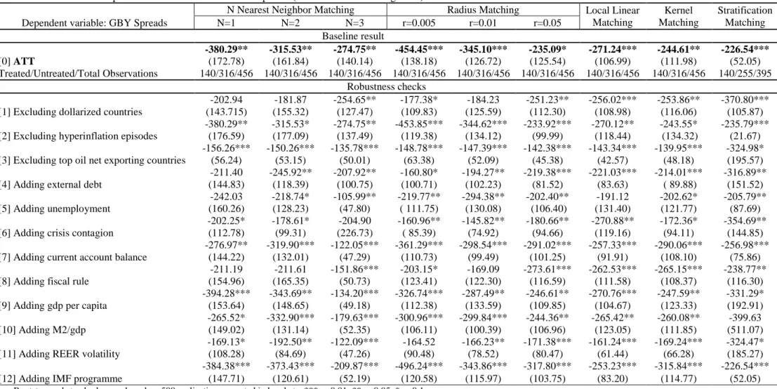
Based on PS estimated in Table 3, we report in Table 4 the estimated ATT of IT adoption on government bond yield spreads, using conservatives starting dates. Our baseline estimations in line [0] show that ATT are negative and statistically significant; thus, IT adoption is found to reduce risk premia on government debt in emerging countries. The size of this effect ranges from 226.54 (for stratification matching) to 454.45 (for a low radius, r=0.005) basis points, and is economically meaningful: IT emerging countries present lower government bond yield spreads, on average between 2 and up to 4.5 pp, compared to countries under monetary or exchange rate targeting.

To check the robustness of our results, we alternatively abstract from dollarized countries, hyperinflation episodes, and top oil exporters (in regressions [1]-[3] in Table 4), and we account for additional determinants of IT adoption (in regressions [4]-[12] in Table 4). Despite some significance loss in some specifications (for example, when excluding dollarized economies in line [1], or when controlling for a fiscal rule in line [8], the ATT is significant in six out of nine cases), the effect of IT adoption on government bond yield spreads is consistent with our results in the baseline specification,18 and it remains so when considering default, instead of conservative IT starting dates (see Appendices 7 and 8).

18 _{In addition, ATT (and their standard errors) for the nearest neighbor matching method, using Abadie et al.}

(2004) to compute standard deviations, are consistent with baseline estimations, namely -223.69 (23.11), -204.30 (32.17), and -192.69 (29.96), for N equal to one, two, and three, respectively.

Table 3. Estimation of PS for Government Bond Yield Spreads (conservative IT starting dates)

[0] Baseline [1] No [2] No [3] No [4] Adding [5] Adding [6] Adding [7] Adding [8] Adding [9] Adding [10] Adding [11] Adding [12] Adding

VARIABLES model dollarized hyperinfl Top oil exp ext debt unempl crisis cont CA balance fiscal rule gdp pc M2/gdp REER vol IMF prog

Lagged inflation -0.115*** -0.116*** -0.115*** -0.080*** -0.108*** -0.115*** -0.113*** -0.119*** -0.110*** -0.116*** -0.129*** -0.104*** -0.104***

(0.0193) (0.0191) (0.0192) (0.0189) (0.0186) (0.0198) (0.0188) (0.0201) (0.0193) (0.0193) (0.0196) (0.0186) (0.0196)

Real gdp growth -0.071*** -0.072*** -0.075*** -0.067*** -0.061*** -0.059*** -0.051** -0.079*** -0.071*** -0.092** -0.075*** -0.086*** -0.045**

(0.0211) (0.0212) (0.0213) (0.0235) (0.0209) (0.0206) (0.0235) (0.0211) (0.0212) (0.0417) (0.0214) (0.0215) (0.0223)

Lagged log total debt/gdp -0.346** -0.353** -0.357** -0.957*** -0.379*** -0.370*** -0.411*** -0.333** -0.355** -0.311** -0.356** -0.486***

(0.142) (0.141) (0.143) (0.180) (0.144) (0.139) (0.139) (0.143) (0.142) (0.152) (0.143) (0.175)

Lagged fiscal deficit -0.082*** -0.079*** -0.083*** -0.136*** -0.035* -0.084*** -0.096*** -0.061** -0.082*** -0.084*** -0.089*** -0.091*** -0.111***

(0.0256) (0.0256) (0.0256) (0.0311) (0.0192) (0.0262) (0.0253) (0.0244) (0.0257) (0.0257) (0.0265) (0.0259) (0.0300)

law and order -0.351*** -0.362*** -0.355*** -0.391*** -0.352*** -0.345*** -0.313*** -0.377*** -0.327*** -0.353*** -0.292*** -0.333*** -0.311***

(0.0732) (0.0742) (0.0735) (0.0831) (0.0734) (0.0706) (0.0739) (0.0703) (0.0778) (0.0728) (0.0786) (0.0757) (0.0756)

Log total exchange reserves 9.165*** 8.794*** 9.210*** 14.20*** 10.44*** 10.18*** 9.695*** 10.63*** 9.005*** 9.109*** 10.78*** 9.204*** 9.922***

(1.144) (1.221) (1.151) (1.600) (1.253) (1.271) (1.179) (1.266) (1.144) (1.148) (1.393) (1.196) (1.424)

Log trade openness/gdp 0.606 0.602 0.700 0.246 0.283 1.046 1.040 0.553 0.619 1.051 0.765 -0.222

(0.684) (0.675) (0.685) (0.786) (0.676) (0.666) (0.676) (0.684) (0.682) (0.706) (0.685) (0.687)

Fixed exchange rate dummy -1.876*** -1.791*** -1.881*** -1.511*** -1.783*** -1.874*** -1.908*** -2.002*** -1.839*** -1.887*** -1.771*** -1.826*** -1.495***

(0.293) (0.314) (0.292) (0.317) (0.260) (0.290) (0.307) (0.310) (0.293) (0.288) (0.291) (0.304) (0.277)

Sovereign debt crisis -1.654* -1.676* -1.309 -1.803** -1.616* -1.488* -1.732* -1.644* -1.730* -1.254 -1.485*

(0.912) (0.921) (0.889) (0.728) (0.897) (0.819) (0.912) (0.916) (0.962) (0.790) (0.771)

Lagged log external debt/gni 0.843**

(0.356)

Unemployment rate 0.443***

(0.142)

Sovereign debt crisis contagion 0.290***

(0.111)

Current account balance -0.0613***

(0.0153)

Fiscal rule 0.210

(0.154)

Log gdp per capita 2.089

(3.475)

Log M2/gdp -0.467**

(0.198)

REER volatility -0.0206

(0.0132)

IMF programme dummy 0.0728

(0.167) Pseudo R2_{/Observations 0.3998/601 0.3717/544 0.3951/587 0.4334/480 0.3988/609 0.4133/601 0.3946/601 0.4198/606 0.4027/601 0.4002/601 0.4080/601 0.3817/571 0.4003/535}

Table 4. ATT of IT adoption on Government Bond Yield Spreads (conservative IT starting dates) Dependent variable: GBY Spreads

N Nearest Neighbor Matching Radius Matching Local Linear Matching Kernel Matching Stratification Matching N=1 N=2 N=3 r=0.005 r=0.01 r=0.05 Baseline result [0] ATT -380.29** -315.53** -274.75** -454.45*** -345.10*** -235.09* -271.24*** -244.61** -226.54*** (172.78) (161.84) (140.14) (138.18) (126.72) (125.54) (106.99) (111.98) (52.05) Treated/Untreated/Total Observations 140/316/456 140/316/456 140/316/456 140/316/456 140/316/456 140/316/456 140/316/456 140/316/456 140/255/395 Robustness checks [1] Excluding dollarized countries

-202.94 -181.87 -254.65** -177.38* -184.23 -251.23** -256.02*** -253.86** -370.80*** (143.715) (155.32) (127.47) (109.83) (125.59) (112.30) (108.98) (116.06) (105.87) [2] Excluding hyperinflation episodes

-380.29** -315.53* -274.75** -453.85*** -344.62*** -233.92*** -270.12** -243.55* -235.79*** (176.59) (177.09) (137.49) (119.38) (134.12) (99.99) (118.44) (134.32) (21.67) [3] Excluding top oil net exporting countries

-156.26*** -150.26*** -135.78*** -148.78*** -147.39*** -142.38*** -143.34*** -139.95*** -324.98* (56.24) (53.15) (50.01) (63.38) (52.09) (45.38) (42.57) (48.18) (195.57) [4] Adding external debt

-211.40 -245.92** -207.92** -160.80* -194.27** -219.38*** -221.03*** -214.01*** -316.89** (144.83) (118.39) (100.75) (100.71) (102.23) (81.52) (83.63) ( 89.88) (151.52) [5] Adding unemployment

-242.03 -218.74* -105.99** -219.77** -294.38** -202.40** -191.12 -202.62* -205.79** (160.26) (128.23) (47.80) ( 111.75) (130.08) (106.40) (131.40) (121.77) (87.69) [6] Adding crisis contagion

-202.25* -178.61* -204.90 -160.96** -145.82** -180.66** -270.88** -172.36* -354.69** (112.78) (99.31) (226.73) ( 85.39) (74.92) (94.66) (119.16) (94.11) (144.85) [7] Adding current account balance

-276.97** -319.90*** -122.05*** -361.29*** -298.54*** -291.02*** -257.33*** -290.06*** -256.98*** (144.22) (132.01) (47.29) (110.73) (99.49) (101.25) (91.91) (108.10) (75.86) [8] Adding fiscal rule

-211.19 -211.61 -151.86*** -203.15* -169.09 -273.61*** -262.53*** -265.15*** -238.77** (154.96) (165.35) (50.73) (123.41) (122.30) (116.59) (111.58) (108.37) (116.30) [9] Adding gdp per capita

-394.28*** -343.69** -134.20*** -326.74*** -287.49** -246.61** -270.76*** -247.59** -331.29* (153.64) (148.65) (49.18) (112.38) (133.59) (109.85) (104.67) (123.33) (192.91) [10] Adding M2/gdp

-265.52* -332.90*** -179.63*** -300.96*** -299.84*** -244.36** -265.42** -260.08** -399.63 (149.02) (131.14) (52.35) (106.11) (100.39) (106.96) (123.05) (111.85) (511.07) [11] Adding REER volatility

-169.13* -192.50** -122.09*** -164.52 -166.23** -171.38*** -161.24*** -169.24*** -324.47* (108.28) (84.69) (47.26) (90.48) (78.52) (80.47) (61.44) (66.28) (185.27) [12] Adding IMF programme

-384.38*** -373.43*** -209.87*** -496.24*** -343.86*** -317.80*** -253.23*** -315.84*** -226.54*** (147.71) (120.61) (52.19) (120.58) (115.97) (103.75) (83.20) (114.77) (52.05)

IV. Sensitivity

Our main results show that IT adoption has a favorable effect on both sovereign debt ratings and government bond yield spreads in the emerging countries in our sample. In the following, we investigate the sensitivity of these findings.

4.1. The quality of the matching

We analyze the robustness of matching result with respect to the two PSM assumptions, namely the common support and the conditional independence.

Regarding the former, the literature suggests different methods for assessing the performance of estimated PS as balanced scores. One commonly-used approach is a t-test of the null hypothesis of the mean between treated and control groups, conditional to estimated PS. Intuitively, after controlling for PS, there should not be any significant difference between treated and untreated observations in the common support area. However, this approach is not immune to criticism. On the one hand, the t-test is computed on observations from the common support, so the result would be sensitive to the matching algorithm (Lee, 2013). On the other hand, the right approach should be based on total sample characteristics (Imai et al., 2008). For these reasons, we follow Sianesi (2004) and re-estimate PS on matched units using a probit model. For each estimated ATT, we report a pseudo R2, defined as the difference between the pseudo R2 for the matched sample and for the unmatched sample. A small pseudo R2 signals that PS can be used as balanced scores. Results in Table 5 for ratings and in Table 6 spreads reveal pseudo R2 fairly close to 0. Thus, our matching allowed obtaining balanced scores, for estimating the treatment effect of IT adoption on both debt ratings and bond yield spreads.

Regarding the latter, the validity of matching estimations is related to the potential influence of non-observable variables. To test this assumption of selection on observables, we use the statistical test of Mantel & Hsenszel (1959).19 This test evaluates how strongly the contribution of non-observable could bias our findings, by testing the null hypothesis that the effect of IT adoption on ratings or spreads is zero. We report the statistic for the upper bound under the assumption that the treatment effect has been overestimated. The results of the test, together with 5 and 10% bounds, show that our findings may be questioned around an odds

19

The Mantel & Hsenszel (1959) statistical test implementation requires a binary outcome variable. Thus, we transform our outcome variables to dichotomous variables, taking a value of 1 if there is a rating upgrade or a decrease in bond yield spread for a given country between two periods, and 0 otherwise. To insure that this transformation does not lead to false conclusions, we re-estimate in each case the ATT of IT with the binary outcome variables (we report that results are consistent with our previous findings).

ratio between 1.85 and 2.7 for sovereign debt ratings (see Table 5), and between 2.35 and 3.9 for government yield spreads (see Table 6). In other words, the estimated effect of IT adoption on sovereign debt ratings and bond yield spreads is robust provided that unobserved variables do not change the odds ratio between treated and control units by more than a factor around 2.5. In light of results highlighted by other studies (for instance, Caliendo & Künn, 2011, concluded with critical values between 1.25 and 3), we can conclude that our findings are fairly robust to the conditional independence assumption.

Table 5. ATT of IT adoption on Sovereign Debt Ratings (conservative IT starting dates): Sensitivity Dependent variable: Sovereign Debt Ratings

Nearest Neighbor Matching Radius Matching Local linear Matching Kernel Matching Stratification Matching N=1 N=2 N=3 r=0.005 r=0.01 r=0.05 Baseline result [0] ATT 2.459** 2.269** 2.257** 2.367*** 2.216*** 2.339*** 2.410*** 2.327*** 2.679*** (0.560) (0.532) (0.453) (0.519) (0.458) (0.363) (0.354) (0.334) (0.558) Treated/Untreated/Total Observations 147/394/541 147/394/541 147/394/541 147/394/541 147/394/541 147/394/541 147/394/541 147/394/541 147/330/477

Testing matching quality: Common support assumption

Pseudo R2 0.047 0.008 0.011 0.007 0.010 0.013 0.015 0.013 0.004

Testing matching quality: Independence conditional assumption MH bounds

p-value=0.05 2.45 1.85 2.1 2 2 1.95 2.15 1.95 2.6

p-value=0.10 2.5 1.9 2.1 2 2 2 2.2 2 2.7

Heterogeneity in treatment effects Comparing IT with Exchange Rate Targeting [14] IT vs Exchange rate targeting

2.537*** 2.601*** 2.582*** 2.750*** 2.328*** 2.420*** 2.489*** 2.395*** 2.424*** (0.594) (0.509) (0.487) (0.583) (0.495) (0.385) (0.368) (0.397) (0.713)

Phase of the business cycle [15] Good times 1.758** 1.855*** 2.172*** 2.685*** 2.449*** 1.617*** 1.828*** 1.656*** 2.007*** (0.771) (0.725) (0.604) (0.943) (0.712) (0.540) (0.509) (0.547) (0.007) [16] Bad times 2.767*** 2.738*** 2.740*** 2.858*** 2.659*** 2.532*** 2.813*** 2.554*** 2.231* (0.693) (0.660) (0.619) (0.879) (0.739) (0.544) (0.482) (0.538) (1.356) Fiscal stance [17] Strong fiscal stance

2.566*** 2.582*** 2.565*** 2.880*** 2.512*** 2.862*** 2.618*** 2.809*** 2.974*** (0.625) (0.569) (0.544) (0.962) (0.728) (0.516) (0.534) (0.515) (0.873) [18] Loose fiscal stance

1.935*** 2.159*** 1.986*** 2.932*** 2.509*** 2.037*** 2.177*** 2.029*** 2.732** (0.933) (0.797) (0.791) (1.065) (0.863) (0.688) (0.684) (0.708) (1.176)

Level of economic development [19] Lower-middle income countries

1.214 1.023 1.182** 1.458 1.782 0.662 0.789 0.715 0.317 (0.727) (0.666) (0.595) (1.429) (1.205) (0.668) (0.620) (0.622) (0.689) [20] Upper-middle income countries

1.181* 1.526*** 1.794*** 1.629*** 1.796*** 1.723*** 1.870*** 1.699*** 1.926*** (0.656) (0.602) (0.560) (0.697) (0.551) (0.485) (0.464) (0.479) (0.049)

Table 6. ATT of IT adoption on Government Bond Yield Spreads (conservative IT starting dates): Sensitivity Dependent variable: GBY Spreads

N Nearest Neighbor Matching Radius Matching Local linear Matching Kernel Matching Stratification Matching N=1 N=2 N=3 r=0.005 r=0.01 r=0.05 Baseline result [0] ATT -380.29** -315.53** -274.75** -454.45*** -345.10*** -235.09* -271.24*** -244.61** -226.54*** (172.78) (161.84) (140.14) (138.18) (126.72) (125.54) (106.99) (111.98) (52.05) Treated/Untreated/Total Observations 140/316/456 140/316/456 140/316/456 140/316/456 140/316/456 140/316/456 140/316/456 140/316/456 140/255/395

Testing matching quality: Common support assumption

Pseudo R2 0.136 0.103 0.065 0.033 0.034 0.048 0.136 0.050 0.047

Testing matching quality: Independence conditional assumption MH bounds

p-value=0.05 2.7 2.85 2.35 3.85 3.35 3.25 3.7 3.25 3.55

p-value=0.10 2.8 2.9 2.4 3.9 3.4 3.3 3.8 3.3 3.6

Heterogeneity in treatment effects Comparing IT with Exchange Rate Targeting [14] IT vs Exchange rate targeting

-308.96* -252.60* -290.63*** -194.39 -205.97* -282.36** -273.06*** -283.77*** -192.31*** (164.92) (151.86) (124.38) (137.50) (127.24) (122.32) (101.34) (107.28) (61.20)

Phase of the business cycle [15] Good times -46.01 -55.94 -75.68** -97.23 -108.90** -73.38** -64.41* -51.13 -165.27*** (49.67) (44.59) (38.97) (69.85) (52.48) (37.09) (35.05) (33.37) (56.73) [16] Bad times -50.23 -56.05 -47.48 -32.61 -37.05 -118.87 -117.13 -112.98 -629.13 (205.41) (172.22) (149.07) (256.33) (187.13) (137.75) (113.41) (128.78) (407.32)

Fiscal policy stance [17] Strong fiscal stance

-78.83* -72.97* -71.24 -109.13* -95.11** -66.58* -88.40*** -66.63* -103.31** (46.53) (41.30) (40.88) (68.81) (49.97) (35.74) (34.60) (37.47) (42.24) [18] Loose fiscal stance

-185.95 -362.17 -274.68 -145.51 -214.97 -281.40 -280.45 -280.57 -549.80 (264.52) (243.88) (207.61) (299.39) (229.68) (214.21) (222.62) (221.25) (493.35)

Level of economic development [19] Lower-middle income countries

-85.48 -138.40 -109.85 -265.19 -255.51 -78.56 -143.04 -88.69 -594.40 (188.94) (161.45) (148.63) (335.47) (303.95) (186.35) (182.64) (191.41) (557.12) [20] Upper-middle income countries

-239.43 -236.56 -315.98* -259.04* -252.97* -357.23** -346.57*** -357.23** -188.84*** (198.81) (169.27) (189.28) (173.11) (158.66) (161.50) (137.64) (166.71) (43.92)

Government Bond Yield Spreads Variability

[21] GBY Spreads variability -56.85 -65.71* -75.97** -59.86* -73.99** -82.10*** -80.95*** -83.62*** -55.50*** (44.92) (36.04) (33.88) (37.32) (31.79) (28.77) (28.70) (31.52) (15.58)

4.2. Heterogeneity of the treatment effect of IT adoption

4.2.1. Sovereign debt ratings

We begin by analyzing the effect of IT adoption on sovereign debt ratings. First, as emphasized by Lin & Ye (2012), exchange rate targeting is a credible and effective monetary strategy in emerging countries. Thus, to compare IT with exchange rate targeting, we exclude fixed exchange rate countries from the control group. The estimated ATT reported in line [14] in Table 5 is positive and still statistically significant. Thus, IT adoption has a favorable effect on sovereign debt ratings in emerging countries, compared to emerging countries under exchange rate targeting.

Second, we look for potential differences in the effect of IT adoption depending on the phase of the business cycle. For example, during recessions, the economy may be in a “liquidity trap”; in this case, the question is not fighting inflation, but rather avoiding a risk of deflation. Indeed, Fraga et al. (2003) state that, given its credibility and transparency, one of the most appealing IT features is its relative flexibility in the presence of shocks. Thus, IT might be effective both in expansion and recession periods. We examine this hypothesis by distinguishing between “good” and “bad” times, such as the former (latter) periods are defined by a positive (negative) output gap.20 Estimations presented in lines [15]-[16] in Table 5 confirm our hypothesis. On the one hand, IT adoption significantly improves sovereign debt ratings both in good and in bad times. However, on the other hand, the estimated ATT are stronger (and even by as much as 1 pp in five out of nine cases) in bad compared to good times: the effect of IT adoption in reducing sovereign debt ratings is more important in bad times, revealing its particular performance against large shocks.

Third, we examine a potential influence of the fiscal stance on the effect of IT adoption on ratings. Indeed, in the presence of a large public debt, the impossibility to resort to seigniorage because of IT can turn a loose fiscal policy into extremely damageable for public debt dynamics (Sargent & Wallace, 1981). This may lead to fiscal dominance, thus making IT less credible. We test this hypothesis by distinguishing between “strong” and “loose” fiscal stance, using the median level of total government debt to separate the two groups. As emphasized by lines [17]-[18] in Table 5, IT adoption has a significant and favorable effect on ratings, irrespective of the fiscal stance. However, IT adoption effectiveness is more pronounced for countries with a strong fiscal stance (in eight out of nine cases), consistent

20 _{Output gap is computed as the difference between actual and potential GDP, and potential GDP is computed}

based on the popular Hodrick-Prescott filter, with a smoothing parameter of 6.25, as suggested by Ravn & Uhlig (2002).

with the conclusions of Lin & Ye (2009). Consequently, by strengthening IT credibility, better policy coordination between fiscal and monetary policies contributes to a higher effect of IT adoption on sovereign debt ratings.

Fourth, macroeconomic performances of emerging countries display substantial heterogeneity. We analyze this potential heterogeneity by distinguishing between “lower-middle income” and “upper-“lower-middle income” countries, based on World Bank’s classification (see Appendices 3 and 4). Estimated ATT reported in lines [19]-[20] in Table 5 show that, unlike its favorable effect in upper-middle income countries, IT adoption does not have a statistically significant effect on ratings in lower-middle income countries. Thus, IT adoption perception differs with the level of economic development, suggesting that financial rating agencies attribute enough credibility to IT adoption in order to modify rates only in relatively more developed countries.

Finally, we equally performed the sensitivity analysis on default, instead of conservative, IT starting dates (see Appendix 9). If most of results are consistent with our previous findings, accounting for IT default dates is no longer associated with strong differences between good and bad times. Only in one out of nine cases the difference equals one rating grade, meaning that a full-fledged IT must be in place for credit rating agencies to value more IT adoption in bad times.

4.2.2. Government bond yield spreads

Let us now turn to the effect of IT adoption on bond yield spreads. First, we compare IT countries to exchange rate targeting countries, by abstracting of fixed exchange rate countries from the control group. As illustrated by line [14] in Table 6, IT adoption significantly decreases bond yield spreads, compared to emerging countries with exchange rate targeting. Second, lines [15]-[16] in Table 6 display estimated ATT for “good” and “bad” times. If some effects are at work in good times, IT adoption had no significant effect on bond yield spreads in bad times in the emerging countries in our sample. Thus, contrary to rating agencies (see line [16] in Table 5), markets do not see IT adoption as a sufficiently binding constraint on debt dynamics in “bad” times, and thus do not mirror this monetary institutional change into significant spreads reductions.

Third, the effect of IT adoption on spreads radically changes with the fiscal stance. On the one hand, adopting IT in a context of strong fiscal stance significantly decreases spreads (see line [17] in Table 6), consistent with its favorable effect on ratings. However, on the other hand, under a loose fiscal stance, IT adoption has no significant impact on spreads (see line [18] in

Table 6), contrary to its favorable effect on ratings. Yet again, markets seem to be more sensitive than rating agencies to the joint behavior of fiscal and monetary policies, as poor fiscal policies inhibit IT credibility from the standpoint of risk-aversion investors.

Fourth, disaggregating the effect of IT adoption on government bond spreads upon the level of economic development leads to findings comparable to its effect on ratings. Contrary to its lack of impact in lower-middle income countries (line [19] in Table 6), IT adoption is found to significantly decrease spreads in upper-middle income countries (line [20] in Table 6). Thus, similar to notation agencies, markets also value IT adoption in relatively more developed emerging countries.

Fifth, we estimate the effect of IT on bond yield spreads variability, defined as the standard deviation of the thirty-six-months moving average of monthly yield spreads level. Results depicted on line [21] in Table 6 show that IT adoption significantly decreases government borrowing cost variability (the estimated ATT is significant in 8 out of 9 cases), and that this decrease is economically meaningful, namely between -55.50 (for stratification matching) and -83.62 (for kernel matching) basis points. Given an average yield variability of 232 basis points in no-IT countries, our findings are that IT adoption can reduce government borrowing cost variability by nearly 30 percent in emerging countries.

Finally, evidence based on default IT starting dates is mostly consistent with results based on conservative dates (see Appendix 10). However, there is an important exception: IT adoption no longer significantly decreases bond yield spreads compared to emerging countries under exchange rate targeting. Corroborated with a previous result that highlighted the benefits of full-fledged IT in bad times, this finding shows that there exist cases in which full-fledged IT perform better than partial IT in terms of sovereign debt risk.

V. Conclusion

We explored in this paper the potential impact of inflation targeting adoption on sovereign debt risk. Our paper contributes to the scarce literature on this topic on several grounds, including (i) alternative measures of sovereign debt risk, (ii) the use of propensity scores matching to control for a self-selection bias in IT adoption, (iii) the use of a large sample of 38 emerging countries, and (iv) a wide analysis of the sensitivity of the effect of IT adoption on sovereign risk, with respect to the phase of the business cycle, the fiscal stance, and the level of economic development.

Our results are as twofold. On the one hand, we find that IT adoption significantly increases sovereign debt ratings and reduces government bond yield spreads. The magnitude of these

effects is economically meaningful: an increase between one and two rating levels, and a decrease between 2 and 4 pp for spreads. These findings are robust to a wide set of alternative specifications for computing propensity scores, including the use of different sub samples or controlling for the determinants of sovereign bond risk previously highlighted in the literature, and they do not depend on the employed matching method. On the other hand, we show that the effect of IT adoption on sovereign debt risk heavily depends on economic conditions. Regarding ratings, IT adoption increases them more during “bad” times and in countries with strong fiscal stance, and significantly increases ratings only in upper-middle income countries. Regarding spreads, IT adoption has no significant effect in “bad” times in countries with loose fiscal stance, and in lower-middle income countries. Our estimations confirm that rating agencies and markets sometimes value differently the adoption of the IT monetary framework, and justify our choice of capturing the diversity of sovereign debt risk through alternative measures.

Consequently, this paper develops the literature on the determinants of sovereign bond risk, by showing that adopting an IT monetary regime can provide benefits in terms of both higher ratings and lower spreads in emerging countries. In addition, our analysis provides insightful evidence on the practical implementation of IT: the highest benefits of IT adoption in terms of reducing sovereign debt risk arise when combined with a good fiscal stance and in relatively more developed emerging countries, provided that a full-fledged IT monetary framework is achieved. Under such conditions, IT adoption can improve emerging market economies’ access to international financial markets, and provide an appropriate monetary strategy to finance long-term investment projects and support potential economic growth.