HAL Id: hal-02985661
https://hal.archives-ouvertes.fr/hal-02985661
Submitted on 28 Apr 2021
HAL is a multi-disciplinary open access
archive for the deposit and dissemination of
sci-entific research documents, whether they are
pub-lished or not. The documents may come from
teaching and research institutions in France or
abroad, or from public or private research centers.
L’archive ouverte pluridisciplinaire HAL, est
destinée au dépôt et à la diffusion de documents
scientifiques de niveau recherche, publiés ou non,
émanant des établissements d’enseignement et de
recherche français ou étrangers, des laboratoires
publics ou privés.
Synthesis and Terrestrial Model Intercomparison
Project – Part 1: Overview and experimental design
D. Huntzinger, C. Schwalm, A. Michalak, K. Schaefer, A. King, Y. Wei, A.
Jacobson, S. Liu, R. Cook, W. Post, et al.
To cite this version:
D. Huntzinger, C. Schwalm, A. Michalak, K. Schaefer, A. King, et al.. The North American Carbon
Program Multi-Scale Synthesis and Terrestrial Model Intercomparison Project – Part 1: Overview
and experimental design. Geoscientific Model Development, European Geosciences Union, 2013, 6
(6), pp.2121-2133. �10.5194/gmd-6-2121-2013�. �hal-02985661�
www.geosci-model-dev.net/6/2121/2013/ doi:10.5194/gmd-6-2121-2013
© Author(s) 2013. CC Attribution 3.0 License.
Geoscientific
Model Development
The North American Carbon Program Multi-Scale Synthesis and
Terrestrial Model Intercomparison Project – Part 1:
Overview and experimental design
D. N. Huntzinger1, C. Schwalm2, A. M. Michalak3, K. Schaefer4,5, A. W. King6, Y. Wei6, A. Jacobson4,7, S. Liu6, R. B. Cook6, W. M. Post6, G. Berthier8, D. Hayes6, M. Huang9, A. Ito10, H. Lei11,12, C. Lu13, J. Mao6, C. H. Peng14,15, S. Peng8, B. Poulter8, D. Riccuito6, X. Shi6, H. Tian13, W. Wang16, N. Zeng17, F. Zhao17, and Q. Zhu15
1School of Earth Sciences and Environmental Sustainability and the Department of Civil Engineering,
Construction Management, and Environmental Engineering, Northern Arizona University, P.O. Box 5694, Flagstaff, Arizona, USA
2School of Earth Sciences and Environmental Sustainability, Northern Arizona University, USA
3Department of Global Ecology, Carnegie Institution for Science, Stanford, California, USA
4National Snow and Ice Data Center, Boulder, Colorado, USA
5Cooperative Institute for Research in Environmental Sciences, University of Colorado, Boulder, Colorado, USA
6Environmental Sciences Division, Oak Ridge National Laboratory, Oak Ridge, Tennessee, USA
7NOAA Earth System Research Lab Global Monitoring Division, Boulder, Colorado, USA
8Laboratoire des Sciences du Climat et de l’Environnement, LSCE, Gif sur Yvette, France
9Fundamental & Computational Sciences, Pacific Northwest National Laboratory, Richland, Washington, USA
10National Institute for Environmental Studies, Tsukuba, Japan
11Atmospheric Sciences and Global Change Division, Pacific Northwest National Laboratory, Richland, Washington, USA
12State Key Laboratory of Hydroscience and Engineering, Department of Hydraulic Engineering, Tsinghua University,
Beijing, China
13International Center for Climate and Global Change Research and School of Forestry and Wildlife Sciences,
Auburn University, Auburn, Alabama, USA
14Department of Biology Sciences, Institute of Environment Sciences, University of Quebec at Montreal,
C.P. 8888, Succ. Centre-Ville, Montreal H3C 3P8, Canada
15Laboratory for Ecological Forecasting and Global Change, College of Forestry, Northwest A&F University, Yangling,
Shaanxi 712100, China
16Ames Research Center, National Aeronautics and Space Administration, Moffett Field, California, USA
17Department of Atmospheric and Oceanic Science, University of Maryland, College Park, Maryland, USA
Correspondence to: D. N. Huntzinger ([email protected])
Received: 24 May 2013 – Published in Geosci. Model Dev. Discuss.: 23 July 2013 Revised: 30 October 2013 – Accepted: 6 November 2013 – Published: 17 December 2013
Abstract. Terrestrial biosphere models (TBMs) have become
an integral tool for extrapolating local observations and un-derstanding of land–atmosphere carbon exchange to larger regions. The North American Carbon Program (NACP) Multi-scale synthesis and Terrestrial Model Intercomparison Project (MsTMIP) is a formal model intercomparison and evaluation effort focused on improving the diagnosis and
attribution of carbon exchange at regional and global scales. MsTMIP builds upon current and past synthesis activities, and has a unique framework designed to isolate, interpret, and inform understanding of how model structural differ-ences impact estimates of carbon uptake and release. Here we provide an overview of the MsTMIP effort and describe how the MsTMIP experimental design enables the assessment and
quantification of TBM structural uncertainty. Model struc-ture refers to the types of processes considered (e.g., nutri-ent cycling, disturbance, lateral transport of carbon), and how these processes are represented (e.g., photosynthetic formu-lation, temperature sensitivity, respiration) in the models. By prescribing a common experimental protocol with standard spin-up procedures and driver data sets, we isolate any biases and variability in TBM estimates of regional and global car-bon budgets resulting from differences in the models them-selves (i.e., model structure) and model-specific parameter values. An initial intercomparison of model structural dif-ferences is represented using hierarchical cluster diagrams (a.k.a. dendrograms), which highlight similarities and differ-ences in how models account for carbon cycle, vegetation, energy, and nitrogen cycle dynamics. We show that, despite the standardized protocol used to derive initial conditions, models show a high degree of variation for GPP, total liv-ing biomass, and total soil carbon, underscorliv-ing the influ-ence of differinflu-ences in model structure and parameterization on model estimates.
1 Introduction
Projections of future climate conditions are based, in part, on the ability to simulate the key drivers and underlying processes that control how atmospheric carbon (primarily
CO2 and CH4)is exchanged with the terrestrial biosphere.
Process-based models (a.k.a. Terrestrial Biospheric Models, TBMs) can be used to attribute carbon sources and sinks to explicit ecosystem processes, and are based on current mech-anistic understanding of how carbon is exchanged with the atmosphere, and allocated or partitioned within ecosystems. Several factors influence the terrestrial carbon uptake and re-lease predicted by models, including a model’s sensitivity to climate, atmospheric composition, and nutrient and water availability. In addition, estimates from TBMs can depend strongly on environmental driver data (Poulter et al., 2011), initial conditions, and parameterizations, as well as which processes controlling carbon exchange are considered and how these processes are formulated (e.g., the functional form used to represent a particular mechanism or process) and scaled within the model. For example, whether (and how) models incorporate land-use and land cover change and other disturbances (e.g., fire) can have a significant impact on a model’s prediction of net land–atmosphere carbon exchange (Liu et al., 2011). As a result, existing estimates of land– atmosphere carbon exchange from TBMs vary widely (e.g., Huntzinger et al., 2012), and coupled-carbon-climate mod-els disagree on the strength of the net land sink (when and
where CO2 uptake through photosynthesis exceeds carbon
losses to the atmosphere), and whether the land surface will
continue to be a net sink of atmospheric CO2under changing
climatic and environmental conditions (e.g., Friedlingstein et al., 2006).
Uncertainties in, or variations among, TBM estimates are driven by a complex combination of assumptions, scien-tific hypotheses, and model choices (Beer et al., 2010). Ide-ally, TBM performance would be assessed by comparing model estimates to available observations. However, there are no direct observations of land–atmosphere carbon flux
at the spatial resolutions (e.g., 0.5◦by 0.5◦) and scales (e.g.,
global) needed to evaluate different model approaches, and thus guide model development and predictions of carbon exchange under future climatic conditions (Melillo et al., 1995; Heimann et al., 1998; McGuire et al., 2010). Thus, it becomes necessary to investigate, at a minimum, how inter-model differences influence variability and therefore uncertainty in results. Multi-model intercomparison projects (MIPs) help to characterize or synthesize current understand-ing of land–atmosphere carbon exchange, and inform the un-certainty or confidence surrounding projections of future ex-change and feedbacks with the climate system.
Past MIPs have shown both the promise of using TBMs to better understand the complex carbon-climate system, as well as the challenges in evaluating model results (e.g., Melillo et al., 1995; Cramer and Field, 1999; Randerson et al., 2009; Schwalm et al., 2010; Huntzinger et al., 2012). In 2008, the North American Carbon Program (NACP) be-gan several interim synthesis activities to evaluate and inter-compare TBMs and observations at site (e.g., Schwalm et al., 2010; Schaefer et al., 2012) and regional scales (e.g., Hayes et al., 2012; Huntzinger et al., 2012).
The site synthesis focused on the comparison of observed
terrestrial CO2 flux from 44 eddy covariance (EC) sites to
site-level simulations from 21 TBMs, and provided a frame-work for evaluating model skill in terms of model
struc-ture, biome-type, and CO2uptake in terms of seasonality and
drought (Schwalm et al., 2010; Schaefer et al., 2012). How-ever, the lack of sensitivity simulations, along with the short timescale of model runs (mean site record length < 5 yr) and the non-representative sample of eddy covariance sites used in the study (e.g., climate regime, ecosystem type), com-plicated diagnosis and attribution of overall model perfor-mance.
The NACP Regional and Continental Interim Synthesis (RCIS) activities, in contrast to the site synthesis, collected existing or “off-the-shelf” simulation results from 19 TBMs (Huntzinger et al., 2012). The decision to use existing results instead of prescribing new simulations was based largely on the need to have a “first look” synthesis of existing, mostly independent TBM results. Thus, the NACP RCIS provided a comprehensive assessment of the range of estimates of land– atmosphere carbon exchange, and by extension the uncer-tainty associated with such estimates, including uncertainties resulting not only from model formulation and assumptions, but also from the choice of environmental driver data and spin up procedure. However, the lack of a detailed simulation protocol and consistent forcing data precluded the attribution
20+ Terrestrial biospheric models (TBMs) Atmospheric CO2 & nitrogen deposi>on Soil proper>es SG1/SR1: • Climatology SG2/SR2: • Climatology • Land-‐use & land-‐cover
change history
SG3/SR3: • Climatology • Land-‐use & land-‐cover
change history • Atmospheric CO2
BG1/BR1: • Climatology • Land-‐use & land-‐cover
change history • Atmospheric CO2
• N Deposi>on Global (SG1,SG2,SG3,BG1) & North America (SR1,SR2,SR3,BR1) Simula=ons
Model
Output Analysis Observa>onally based data
Phenology
Climatology C3/C4 grass & major crops
Land-‐use & land-‐cover change history
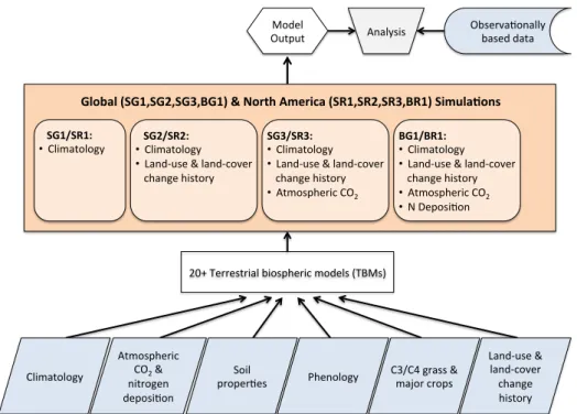
Fig. 1. Schematic of the Multi-Scale Synthesis and Terrestrial Model Intercomparison Project (MsTMIP) framework. Global simulations (SG1,SG2, SG3,BG1) are run at 0.5◦by 0.5◦resolution; North American simulations (SR1, SR2, SR3, BR1) are run at 0.25◦by 0.25◦ resolution).
of observed across-model variability to differences in mod-eling approaches.
While the NACP RCIS and Site syntheses efforts provided a unique forum for summarizing the status of terrestrial car-bon modeling, they also reinforced the need for a consistent and unified model evaluation framework in order to isolate, interpret, understand, and better address differences – pri-marily structural or process representations – among state-of-the-art TBMs simulating land–atmosphere exchange over continental to global extents.
This manuscript provides an overview of, and describes the experimental protocol for, the Multi-Scale Synthesis and Terrestrial Model Intercomparison Project (MsTMIP). The MsTMIP activity was created to build off of and complement recent and ongoing synthesis efforts such as the NACP RCIS and site interim synthesis activities described above, as well as the Trends in Net Land-Atmosphere Carbon Exchange
(TRENDY1), the regionally focused Large Scale Biosphere
Atmosphere-Data Model Intercomparison Project
(LBA-MIP2), and the International Land-Atmosphere
Benchmark-ing Project (ILAMB3; a framework confronting coupled
carbon-climate models with data). The goal of MsTMIP
1http://dgvm.ceh.ac.uk/node/21.
2http://www.climatemodeling.org/lba-mip/. 3http://www.ilamb.org/.
is to quantify, within a unified intercomparison frame-work (Fig. 1), the contribution of model structural dif-ferences to across-model variability in estimates of land– atmosphere carbon exchange, thus providing the critical syn-thesis, benchmarking, evaluation, and feedback needed to improve the current state of the art in carbon cycle model-ing. The MsTMIP experimental protocol specifies standard model inputs, simulations and simulation setup procedures, as well as required model output and format to ensure a valid and fair comparison of model results against one another and against available observations. In this paper, we outline some of the key components of the MsTMIP experimental design, focusing on the participating models, key simulations, and spin-up criteria, and show how the initial steady-state results demonstrate the importance of the choices made in the ex-perimental design.
2 MsTMIP experimental design 2.1 Overview
The MsTMIP experimental design includes simulations run
at two spatial resolutions (0.5◦and 0.25◦) and for two
spa-tial domains (globally and regionally over North America) in order to assess model performance at scales relevant to carbon management and climate change predictions. The
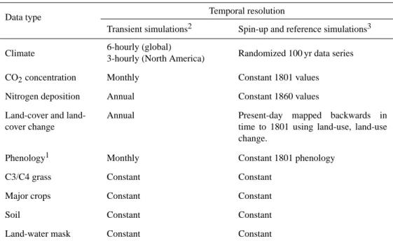
Table 1. Prescribed environmental driver data sets for MsTMIP simulations.
Data type Temporal resolution
Transient simulations2 Spin-up and reference simulations3 Climate 6-hourly (global) Randomized 100 yr data series
3-hourly (North America)
CO2concentration Monthly Constant 1801 values Nitrogen deposition Annual Constant 1860 values Land-cover and
land-cover change
Annual Present-day mapped backwards in time to 1801 using land-use, land-use change.
Phenology1 Monthly Constant 1801 phenology
C3/C4 grass Constant Constant
Major crops Constant Constant
Soil Constant Constant
Land-water mask Constant Constant
1Some models (e.g., CLM4, CLM4VIC) do not use prescribed phenology but rather simulate phenology (e.g. LAI and fPAR)
internally within the model.2Transient simulations (SG1, SG2, SG3, BG1, SR1, SR2, SR3, & BR1).3Spin-up driver data package for
model spin-up and for the reference simulations (RG1 & RR1). factors that influence the spatial and temporal evolution of carbon sources and sinks vary across the globe. Thus, global simulations are needed for comparing TBM results with
atmospheric CO2 constraints, while North American (i.e.,
continental-scale) simulations provide the necessary linkage with more well–characterized land-based observational data sets. In addition, the global and North American simulations are linked to two distinct sets of standardized environmental driver data (Wei et al., 2013) in order to test the influence of both spatial resolution and changing driver data on model estimates.
Building off of lessons learned from the NACP interim synthesis activities, one of the primary goals of the MsTMIP activity is to quantify and assess the impact of TBM struc-tural variability, and therefore uncertainty, by examining how inter-model differences influence variability among model results. Structural uncertainty results from differences across models in their representation (or lack of representation) of biogeochemical and biophysical processes. Although struc-tural uncertainty can be quantified, in part, for a given model through a series of sensitivity simulations, it is best quanti-fied through a MIP. To do so, however, a large ensemble of models is needed to span the range of biogeochemical and biophysical process representations, and the simulation pro-tocol must isolate structure, at least to the extent possible, by holding constant as many aspects of simulating the terrestrial carbon cycle as feasible except for the models themselves. Using a MIP in this way cannot truly separate parametric and structural uncertainty, as different model structures will have different parameters, and models with the same process
representations might use different parameter values. Nev-ertheless, if properly designed, observed inter-model differ-ences can be representative of structural difference in model representation, and thus complement parametric uncertainty analyses applied to a single model.
The ability to identify particular structural contributions to inter-model variance can inform areas for model refinement and improvement, particularly if the model differences are evaluated against observation-based benchmarks of model performance (e.g., Luo et al., 2012). As such, in addition to prescribing simulations over two spatial scales and domains, the MsTMIP experimental design includes four key compo-nents to help attribute variability in model results to inter-model differences.
First, to ensure consistent and comparable model results, the MsTMIP simulations are performed using a consistent set of environmental driver data, including standard climate and atmospheric drivers, remotely sensed phenology, biome clas-sification, and land-use history (Table 1). The rationale for the choices and the preparation of these environmental driver data products are described in detail in Wei et al. (2013).
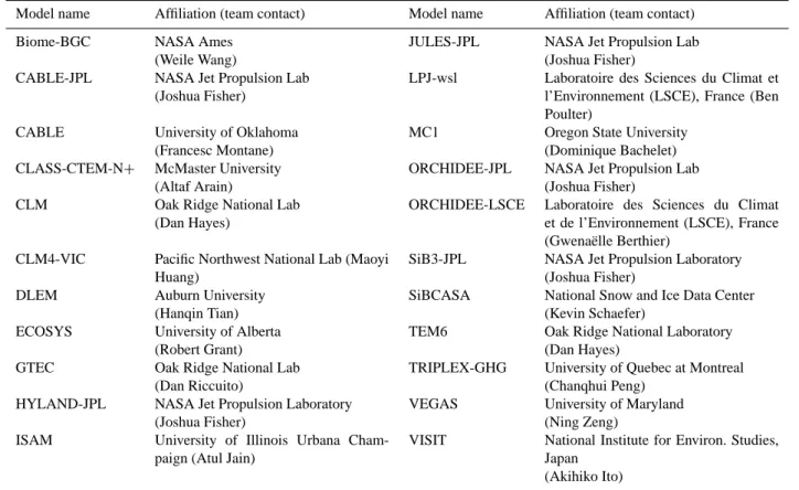
Second, MsTMIP includes over 20 different global-scale TBMs (Table 2), representing the range of model types and complexity (e.g., dynamic versus static vegetation, prognos-tic versus diagnosprognos-tic phenology, various treatments of distur-bance events) used by the scientific community. A broad set of models is needed to gain greater insight into community-wide strengths and weaknesses in TBM model estimates, thus providing insights into the science beyond individual, potentially idiosyncratic, model properties.
Table 2. Terrestrial biospheric models participating in the MsTMIP activity.
Model name Affiliation (team contact) Model name Affiliation (team contact) Biome-BGC NASA Ames
(Weile Wang)
JULES-JPL NASA Jet Propulsion Lab (Joshua Fisher)
CABLE-JPL NASA Jet Propulsion Lab (Joshua Fisher)
LPJ-wsl Laboratoire des Sciences du Climat et l’Environnement (LSCE), France (Ben Poulter)
CABLE University of Oklahoma (Francesc Montane)
MC1 Oregon State University (Dominique Bachelet) CLASS-CTEM-N+ McMaster University
(Altaf Arain)
ORCHIDEE-JPL NASA Jet Propulsion Lab (Joshua Fisher)
CLM Oak Ridge National Lab (Dan Hayes)
ORCHIDEE-LSCE Laboratoire des Sciences du Climat et de l’Environnement (LSCE), France (Gwenaëlle Berthier)
CLM4-VIC Pacific Northwest National Lab (Maoyi Huang)
SiB3-JPL NASA Jet Propulsion Laboratory (Joshua Fisher)
DLEM Auburn University (Hanqin Tian)
SiBCASA National Snow and Ice Data Center (Kevin Schaefer)
ECOSYS University of Alberta (Robert Grant)
TEM6 Oak Ridge National Laboratory (Dan Hayes)
GTEC Oak Ridge National Lab (Dan Riccuito)
TRIPLEX-GHG University of Quebec at Montreal (Chanqhui Peng)
HYLAND-JPL NASA Jet Propulsion Laboratory (Joshua Fisher)
VEGAS University of Maryland (Ning Zeng)
ISAM University of Illinois Urbana Cham-paign (Atul Jain)
VISIT National Institute for Environ. Studies, Japan
(Akihiko Ito)
Table 3. Series of MsTMIP simulations.
Domain Name Time period Climate forcing Land-use history Atmospheric CO2 Nitrogen deposition
Global (0.5◦by 0.5◦) RG1 1901–2010 Constant Constant Constant Constant SG1 CRU+NCEP1 SG2 Time-varying SG3 Time-varying BG1 Time-varying North America (0.25◦by 0.25◦) RR1 1901–2010 Constant Constant Constant Constant SR1 NARR2 SR2 Time-varying SR3 Time-varying BR1 Time-varying
1Climate Research Unit (CRU) + National Centers for Environmental Prediction (NCEP) global climatology.2North American Regional Reanalysis (NARR) climatology.
Third, land–atmosphere carbon exchange is modeled over a 110 yr period using a series of sensitivity simulations (Ta-ble 3), which allow for a robust assessment of model
sensi-tivity to forcing factors such as climate, atmospheric CO2,
nitrogen, and land cover change. The ability to characterize
the contribution of processes such as climate variability, CO2
fertilization, and historical land use and disturbance on car-bon stocks and net ecosystem exchange (NEE) is fundamen-tal to understanding model representations of the terrestrial carbon cycle.
Fourth, the MsTMIP activity includes a systematic eval-uation of model performance against available observation-based products in order to identify strengths and weaknesses within models and guide model development. Although di-rect (gridded) comprehensive observations of carbon fluxes and stocks do not exist, site level data (e.g., eddy covariance observations), inventory data (e.g., forest carbon stocks), regional gridded observations (e.g., aboveground biomass) and model-data products (e.g., data-driven spatially dis-tributed GPP products) can be used to evaluate TBM model
results. Comparing model predictions with available obser-vations and data-driven products can help identify knowl-edge/information gaps in both the models and the obser-vations, and advance process-level understanding of land– atmosphere carbon exchange (US CCSP, 2011). This may ul-timately lead to observing systems that are better optimized for evaluating model performance, as well as encouraging models to generate output that can be more directly com-pared with available observations.
2.2 Participating models
Over 20 TBMs (Table 2) with varying complexity and formu-lations are participating in the MsTMIP activity. This broad suite of models maximizes the degree to which insights can be gained into the uncertainties associated with TBM esti-mates of land–atmosphere carbon exchange. Models vary in complexity and the way in which they simulate canopy con-ductance (energy and water fluxes), simulate photosynthe-sis and respiration (carbon fluxes), allocate carbon between soil and above- and belowground biomass (carbon pools), and model vegetation dynamics and disturbances. In order to track differences in model structure and parameterizations among models, each participating modeling team completed a detailed survey specifying how their model simulates en-ergy and water cycling, as well as carbon and vegetation dy-namics. The results from these surveys can be used to iden-tify key structural differences among the participating mod-els.
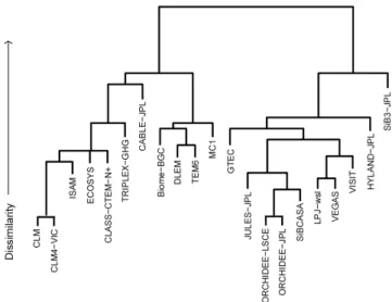
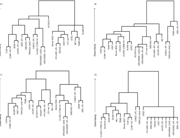
A hierarchical cluster analysis was performed on model structural attributes in order to provide a high-level visual-ization of the similarities and differences among the partici-pating models, (Figs. 2 and 3). For a given characteristic (i.e., process/attribute), a model was assigned a binary value (0 or 1) indicating whether it includes that particular characteris-tic. Thus, for each characteristic or component of the model survey, a model was given a value of one (1) if it considers or includes that process, or a zero (0) if it does not (refer to Ta-bles S1–S4 in the Supplement). The Hamming distance (the number of “mismatches”; Hamming, 1950) was then calcu-lated between the coded integer values for each model pair. Cluster analysis, represented as dendrograms, sorts the mod-els into groups by the level of similarity between modmod-els; models in the same branch in the cluster tree share similar attributes. Separate dendrograms were generated comparing the similarities/differences in models overall (Fig. 2), as well as how they compare in their treatment of energy, vegeta-tion, carbon, and nitrogen dynamics (Fig. 3). Dendrograms provide a means to easily compare overall model similari-ties and differences in a way that is not possible with lengthy tables summarizing various model attributes.
For the purposes of this manuscript, the dendrograms help to illustrate the range of model types and complexities in the models participating in the MsTMIP activity. For example, the models vary widely in how they formulate the energy
23
Figure 2 Fig. 2. Dendrogram showing overall model structural differences
determined by Hamming distance for the models participating in MsTMIP. Models in the same “tree” share similar structural model characteristics. For example, models in the “tree” to the left include an explicit nitrogen cycle, while models in the “tree” to the right do not. Models are further separated or clustered by their treatment of soil carbon pools (e.g., SiB3-JPL does not include live, soil, or litter carbon pools) and their treatment of radiation and canopy heat stor-age (e.g., Biome-BGC, DLEM, TEM6, and MC1 do not account for canopy heat storage, nor partition radiation into latent and sensible heat). Refer to the Supplement for the binary data used to create this diagram.
cycle, including how they simulate canopy and stomatal con-ductance and partition net radiation between latent and sen-sible heat (Fig. 4a). All models account for energy fluxes, but do so in somewhat different ways. Conversely, not all mod-els explicitly consider nitrogen cycling. Hence, two general “trees” of models appear, those that include interactive N cy-cling (e.g., Biome-BGC, DLEM, TEM6, CLM, CLM4VIC, TRIPLEX-GHG), and those that do not (e.g., SIBCASA, ORCHIDEE-LSCE, VEGAS, LPJ-wsl) (Fig. 4d). This di-versity in model structure is needed to provide insights into our ability, as a modeling community, to simulate land– atmosphere carbon dynamics.
2.3 Simulation protocol
Simulations are performed at two spatial scales and
reso-lutions: (1) globally at 0.5◦×0.5◦ spatial resolution; and
(2) over North America at 0.25◦×0.25◦resolution. The
spa-tial extent of the North America region is defined as 50◦to
170◦West longitude and 10◦to 84◦North latitude.
Each simulation runs from 1801 to 2010 and is divided into a common spin-up period (1801–1900) and a sub-mission period (1901–2010). For model spin-up, a spin-up driver data package was created that includes 100 yr of ran-domized weather, time-invariant preindustrial atmospheric
24
Figure 3Fig. 3. Dendrogram showing general differences/similarities in how MsTMIP models formulate and parameterize (A) energy, (B) carbon, (C) vegetation, and (D) nitrogen process dynamics. Clusters are determined by Hamming distance. Models in the same “tree” share similar structural model characteristics. For example, models in the “tree” to the left (e.g., ISAM, CABLE-JPL, ORCHIDEE-JPL/LSCE) in (A) simulate ground heat flux and canopy heat storage, while models in the “tree” to the right (e.g., MC1, TEM6, VEGAS) do not. A majority of models separate live carbon into various pools (with exception of SiB-JPL), but they do so in various ways (e.g., left “tree” in (B)). Refer to the Supplement for the binary data used to create this diagram.
CO2concentrations and nitrogen deposition rates, land-cover
classification and phenology (Table 1; Wei et al., 2013). At the start of spin-up, each model’s prognostic soil, canopy, and canopy air space temperatures are initialized to the average air temperature from the time period 1901 to 1930. Prognos-tic soil moisture variables at all soil levels are initialized to 95 % of saturation, while carbon and nitrogen pools are ini-tialized as needed for each model.
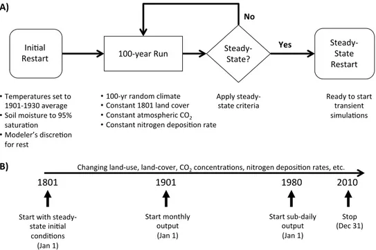
To minimize differences in model output due to differ-ences in initial conditions, all transient simulations start from steady-state initial conditions in 1801, but models submit output only for the submission period (1901–2010). Steady-state conditions are defined as the lack of a trend in prognos-tic variables during the 100 yr spin-up period (1801–1900). The steady-state criteria for the last 100 yr of spin-up for prognostic soil temperature, soil moisture, and carbon flux are shown below and in Fig. 4a. Carbon flux depends on biomass, so the steady-state criterion for carbon flux implic-itly requires that simulated carbon pools also be in equilib-rium. The steady-state criteria are defined as follows:
1. For the carbon cycle, the 100 yr mean interannual change (trend) in total ecosystem carbon stocks for
consecutive years must be below 1 g m−2yr−1 for
95 % of grid cells.
|1Ceco| ≤1 g m−2yr−2.
2. For soil temperature and soil moisture, the 100 yr trend in soil moisture and temperature should not be signifi-cantly different from zero (α = 0.05) for at least 95 % of grid cells.
Reference simulations (i.e., extended spin-up runs, RG1, RR1) are used to track model drift; and given that initial steady-state conditions can, and likely will, vary with model structure, the MsTMIP reference simulations enable exami-nation of how steady-state conditions vary across models. A series of sensitivity simulations (SG1, SG2, SG3, SR1, SR2, SR3) are used to systematically test the additive influence of different forcing factors (i.e, climate (SG1, SR1), land-use
1801 1901 1980 2010
Start with steady-‐ state ini4al condi4ons (Jan 1) Start monthly output (Jan 1) Start sub-‐daily output (Jan 1) Stop (Dec 31) Ini4al Restart Steady-‐ State Restart 100-‐year Run Steady-‐ State?
No
Yes
• Temperatures set to 1901-‐1930 average • Soil moisture to 95%
satura4on • Modeler’s discre4on
for rest
• 100-‐yr random climate • Constant 1801 land cover • Constant atmospheric CO2
• Constant nitrogen deposi4on rate
Apply steady-‐
state criteria Ready to start transient simula4ons
Changing land-‐use, land-‐cover, CO2 concentra4ons, nitrogen deposi4on rates, etc.
A)
B)
Fig. 4. Schematic of (A) the spin-up procedure to steady state; and (B) the basic timeline for each MsTMIP simulation starting from steady-state conditions reached in (A). All transient simulations (B) run from 1801 through 2010 (210 yr). The same initial conditions are used for both the global and North American simulations.
SR3), and nitrogen deposition (BG1, BR1) on model esti-mates of carbon stocks and fluxes. Differences between the various simulations provide insight into the effects of a par-ticular process (e.g., nutrient limitation) or time-varying
en-vironmental drivers (e.g., atmospheric CO2 concentration)
on model output. The “baseline” simulations (BG1, BR1) represent a model’s best estimate of carbon exchange, with everything in the model essentially “turned-on” (Table 3). All simulations (baseline and sensitivity) follow the same spin-up procedure and begin from the same (but model-specific) steady-state conditions (Fig. 2b). Parameter values are not specified as part of the MsTMIP experimental protocol, thus all models are run with their model-specific parameteriza-tions.
2.4 Treatment of disturbance in MsTMIP
Disturbances transfer carbon from one pool to another (e.g., live carbon to dead carbon pools; terrestrial to atmospheric pools), and can alter forest structure (e.g., succession) and biogeochemistry (e.g., by altering soil conditions). Liu et al. (2011) highlight the importance of disturbances such as wildland fire, insect infestation, storms, and harvest on the terrestrial carbon cycle over a range of spatial and temporal scales. Understanding the role of disturbance events and their impacts is therefore critical for improving the quantification of carbon stocks and land–atmosphere carbon fluxes (Liu et al., 2011; Hayes et al., 2011); however, the current capability
for robustly simulating disturbance events (and their impacts) in TBMs is limited (Liu et al., 2011). Although more work is needed in structural development and parameterization of TBMs for incorporating multiple disturbances, the limitation is probably more due to the lack of globally consistent and comprehensive data sets on historical disturbances and their future projections. Because of the lack of robust data sets on disturbance history, disturbance is not explicitly accounted for in the MsTMIP simulation protocol. Instead, models par-ticipating in MsTMIP deal with disturbances in their simu-lations as they normally would, and report their treatment of disturbance in the model surveys discussed in Sect. 2.2. For example, some of the models participating in MsTMIP (e.g., CLM, CLM4VIC, MC1) include disturbances such as fire prognostically (i.e., predictively), while others require a di-agnostic forcing data set (e.g., TEM6, DLEM) or account for fire disturbance implicitly (e.g., through land-cover change history and remotely sensed vegetation indices) rather than explicitly.
2.5 Output
The output variables for each simulation are listed in Ta-ble S5 (refer to the Supplement). VariaTa-bles are grouped into general categories such as carbon and energy fluxes, car-bon pools, and physical variables. When applicable, variable
names and units adhere to the ALMA standard4, and carbon cycle variable definitions follow those outlined by Chapin et al. (2006). The use of common output variable definitions is critical not only for comparing results among the TBMs, but also for comparing carbon flux estimates to those derived
from other modeling approaches (e.g., atmospheric CO2
in-versions). This is particularly true for derived, summary-level carbon flux indicators, such as net ecosystem exchange (NEE) and net ecosystem carbon balance (NECB), that can be compared among different approaches across all spatial and temporal scales (Hayes and Turner, 2012). Because of structural variations, TBMs will differ in terms of which component fluxes are included in these summary-level esti-mates. Here, modeling teams are asked to make their “best guess” for these indicators, as allowed by their particular model and with the requirement of full transparency in the component fluxes included in each calculation. For both the global and North American simulations, monthly model out-put is compiled for the period 1901 to 2010. In order to
com-pare model estimates with atmospheric CO2 concentration
and FLUXNET data, carbon and energy fluxes are also col-lected at 3-hourly intervals for the time period of 1980 to 2010 for the reference (RG1, RR1) and baseline (BG1, BR1) simulations. For some models, however, generating 3-hourly output was not feasible. Thus, for these models, carbon and energy fluxes were collected at the finest temporal resolution possible for that model over the final 30 yr of MsTMIP sim-ulations.
All model submission files are CF-1.x compliant netCDF (version 3), using the standard variable names and units as listed in Table S6. The CF (Climate and Forecast) standards for writing netCDF files are described in extensive online
documentation5. In past efforts (e.g., NACP RCIS and Site
Synthesis), reformatting model output to a common format required significant time and effort. To avoid this problem, a library of output subroutines written in Fortran90 was cre-ated that makes it possible to write model output directly in the required submission file format. These subroutines can be inserted directly in the model code or used in a separate post-processing program. The submission file subroutines with complete user’s guide and documentation are available from
the MsTMIP SVN server6.
3 Preliminary results
This section presents preliminary results from a subset of models participating in MsTMIP, with all results based on the RG1 simulations. Finalized MsTMIP data products will be archived at the ORNL DAAC (http://daac.ornl.gov).
4http://www.lmd.jussieu.fr/~polcher/ALMA/convention_ output_2.html. 5http://cf-pcmdi.llnl.gov/. 6https://edss-collab.ornl.gov/mstmip/svn/nc_output_routines_ fortran. 26 Figure 5
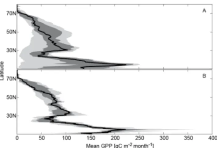
Fig. 5. North American multi-year mean (2000–2005) GPP from (A) the NACP regional and continental interim synthesis (RCIS) and (B) the MsTMIP simulations for 5 models (CLM, DLEM, LPJ-wsl, ORCHIDEE-LSCE, and VEGAS). On each panel, the solid line shows the median of the multi-model ensemble, the darker shaded area shows the interquartile range; and the lighter band shows the full range in estimates.
In order to evaluate the effectiveness of the MsTMIP ex-perimental design in isolating model structural differences while controlling for other sources of variability (i.e., driver data, simulation protocol), we compare the some of the ini-tial model results from the MsTMIP standardized proto-col (Fig. 5b) to results from the NACP RCIS (Fig. 5a), an “unconstrained” protocol (varying environmental driver data, initial conditions, and spatial and temporal resolutions). Steady-state conditions for the NACP RCIS are not available, and we therefore compared the latitudinal gradients of multi-year mean gross primary productivity (GPP) from 2000 to 2005 for the five models (CLM, DLEM, LPJ, ORCHIDEE-LSCE, and VEGAS) common to both synthesis activities. Analogous results across all models participating in either activity (but not necessarily both) are presented in Fig. S1 (see Supplement).
As expected, there is less spread in MsTMIP results than those from the RCIS. Figure 5 shows, that by removing some of the sources of variability (i.e., choice in driver data, spin-up procedure), the variability in model output is reduced, thus demonstrating the importance of the choices made in the experimental design. One reason for the decrease in vari-ability in modeled GPP between the RCIS and MsTMIP in
certain regions (e.g., topics or ∼ 10◦to 30◦N in North
Amer-ica; Fig. 5) could be related to the quality control measures taken in preparing the environmental driver data sets for the MsTMIP activity (Wei et al., 2013). For example, known positive biases in downward shortwave radiation found in the NCEP/NCAR (Kalnay et al., 1996) were removed in the fused CRU-NCEP product created for MsTMIP (Wei et al., 2013), and as shown by Kennedy et al. (2010), biases in ra-diation can have a strong impact on model estimates of GPP.
27
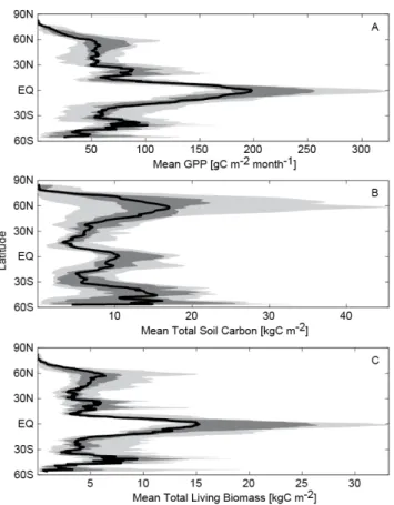
Figure 6 Fig. 6. Global steady-state GPP, total soil carbon, and total living
biomass for 10 MsTMIP models (Biome-BGC, CLM, CLM4VIC, GTEC, LPJ-wsl, ORCHIDEE-LSCE, TRIPLEX-GHG, VEGAS, and VISIT) from the RG1 simulation. The solid black line shows the median of the multi-model ensemble, the darker grey shaded area shows the interquartile range; and the lighter grey band shows the full range in estimates.
Thus by removing known errors in environmental driver data and providing models with consistent driver data and ini-tial conditions, the MsTMIP protocol isolates the impact of model structure on inter-model variability.
Despite the standardized protocol used to derive steady-state conditions, models show a high degree of variation for GPP, total living biomass, and total soil carbon (Fig. 6), un-derscoring the influence of differences in model structure on model estimates. For example, steady-state GPP estimates in the tropics vary by a factor greater than two (Fig. 6a), initial soil carbon pool sizes in the northern high latitudes
ranges widely from 5–45 kg C m−2(Fig. 6b), and total living
biomass (Fig. 6c) varies by a factor of three in the tropics. The degree of variability is of course lower when comparing the interquartile range in order to remove any outliers (darker shaded region in Fig. 6), but the remaining inter-model dif-ferences still remain, particularly in the tropics and northern high latitudes.
28
Figure 7
Fig. 7. Global aggregated steady-state GPP versus total soil carbon, and total living biomass for MsTMIP models from RG1 simulation.
The models also exhibit a high degree of variability in their steady-state, mean annual global totals: GPP ranges from 73
to 165 Pg C yr−1, soil carbon from 405 to 2120 GtC, and
to-tal living biomass from 544 to 1120 GtC. For soil carbon, some of this inconsistency is related to soil depth speci-fied in the models (varies from 1 to 6 m). However, models with shallower soil profiles do not necessarily exhibit smaller pool sizes. Much of the variability in pool size (total liv-ing biomass and total soil carbon) can be linked to differ-ences in GPP among the models (Fig. 7). Models that predict greater global annual carbon uptake generally show larger overall pool sizes. As in the NACP RCIS and Site Synthesis (Huntzinger et al., 2012; Schaefer et al., 2012), variability in model estimates appears to be strongly driven by variability in GPP, or how carbon uptake dynamics are simulated within the models. By isolating some of the sources of variability, MsTMIP’s experimental design will allow for the evalua-tion of model results in a way that was not possible with the NACP RCIS activity.
4 Planned analysis
TBM model-data evaluation, or benchmarking, is one of the core components of the MsTMIP activity. Benchmark-ing can be defined as the organized evaluation of system performance against defined references or observations (i.e., benchmarks) (Luo et al., 2012) with the goal of diagnosing system strengths and deficiencies in order to guide model improvements. Given the complexity of models and the shortage of observational data products at the spatial and temporal resolution of model estimates, it is not possible to independently evaluate each of the modeled processes (Luo et al., 2012). There is often an inconsistency between observations and models in terms of the variables being
measured/simulated, as well as the temporal and/or spatial resolution of the models compared to those of observations. Thus, the alternative is to use some combination of model-model comparisons, comparisons of model-model output to related observations at relevant scales; and the comparisons of model output to equivalent variables/observations at somewhat mis-matched scales. In recognition of these challenges, the MsT-MIP benchmarking activities will emphasize a combination of benchmarking approaches, including site eddy-covariance data (e.g., NEE, latent heat, sensible heat), regional products (e.g., aboveground biomass; Saatchi et al., 2011) and gridded model-data products (e.g., upscaled GPP from Jung et al., 2011). The model-model and model-data comparisons will target scientific questions such as: What are the dominant controls (e.g., climate, land-use, atmospheric conditions) on model estimates of global net land–atmosphere carbon ex-change? What drives the variability observed in model esti-mates of GPP, and how do biases in GPP influence model estimates of net ecosystem exchange?
In addition, methods to evaluate model structural dif-ferences, similar to the dendrograms presented in this manuscript, will be used to attribute differences in estimates between subsets of models to differences in model struc-ture. For example, do model estimates of global long-term mean GPP cluster similarly to model structural attributes? Such side-by-side comparisons will inform understanding of the drivers to inter-model differences in estimates of carbon fluxes and carbon pools. By better understanding the vari-ability that emerges due to structural differences among the models, the MsTMIP activity can help inform understand-ing of what modelunderstand-ing structural choices or assumptions lead to improved model estimates. At a minimum, understanding how structural differences drive inter-model spread can help inform our understanding of model uncertainty, particularly when a discriminating choice among candidate results (e.g., which model is “best”) cannot be made due to lack of avail-able evaluation/validation data.
5 Conclusions and outlook
This paper provides an overview of the experimental design of the Multi-Scale Synthesis and Terrestrial Model Inter-comparison Project (MsTMIP), which is being undertaken as part of the North American Carbon Program. The goal of MsTMIP is to provide, within a unified intercomparison framework, the critical synthesis and feedback needed to improve carbon cycle modeling, and quantify the contribu-tion of model structural differences to inter-model variabil-ity. MsTMIPs experimental design, along with the large suite (20+) of participating models will provide greater insight into community-wide strengths and weaknesses. In addition, the use of a consistent environmental driver data and the combination of simulations makes it possible to isolate the influence of model structural differences on model results.
Understanding how inter-model differences influence vari-ability or uncertainty in model results is necessary for quan-tifying the uncertainty associated with future projections of coupled-carbon-climate feedbacks.
Supplementary material related to this article is available online at http://www.geosci-model-dev.net/6/ 2121/2013/gmd-6-2121-2013-supplement.pdf.
Acknowledgements. Funding for this project was provided through
NASA ROSES Grant # NNX10AG01A. Data management sup-port for preparing, documenting, and distributing model driver and output data was performed by the Modeling and Synthe-sis Thematic Data Center at Oak Ridge National Laboratory (http://nacp.ornl.gov), with funding through NASA ROSES Grant # NNH10AN68I. Finalized MsTMIP data products will be archived at the ORNL DAAC (http://daac.ornl.gov). This is MsTMIP con-tribution #1. Acknowledgments for specific MsTMIP participating models follow.
Biome-BGC: Biome-BGC code was provided by the
Numer-ical Terradynamic Simulation Group at University of Montana. The computational facilities provided by NASA Earth Exchange at NASA Ames Research Center.
CLM: This research is supported in part by the US Department
of Energy (DOE), Office of Science, Biological and Environmen-tal Research. Oak Ridge National Laboratory is managed by UT-BATTELLE for DOE under contract DE-AC05-00OR22725.
CLM4-VIC: This research is supported in part by the US
Depart-ment of Energy (DOE), Office of Science, Biological and Environ-mental Research. PNNL is operated for the US DOE by Battelle Memorial Institute under Contract DE-AC06-76RLO1830.
DLEM: The Dynamic Land Ecosystem Model (DLEM)
devel-oped in the International Center for Climate and Global Change Research at Auburn University has been supported by NASA In-terdisciplinary Science Program (IDS), NASA Land Cover/Land Use Change Program (LCLUC), NASA Terrestrial Ecology Pro-gram, NASA Atmospheric Composition Modeling and Analysis Program (ACMAP); NSF Dynamics of Coupled Natural-Human System Program (CNH), Decadal and Regional Climate Prediction using Earth System Models (EaSM); DOE National Institute for Climate Change Research; USDA AFRI Program and EPA STAR Program.
LPJ-wsl: This work was conducted at LSCE, France, using a
modified version of the LPJ version 3.1 model, originally made available by the Potsdam Institute for Climate Impact Research.
ORCHIDEE-LSCE: ORCHIDEE is a global land surface model
developed at the IPSL institute in France. The simulations were per-formed with the support of the GhG Europe FP7 grant with comput-ing facilities provided by “LSCE” or “TGCC”.
TRIPLEX-GHG: TRIPLEX-GHG developed at University of
Quebec at Montreal (Canada) and Northwest A&F University (China) has been supported by the National Basic Research Pro-gram of China (2013CB956602) and the National Science and En-gineering Research Council of Canada (NSERC) Discover Grant.
VISIT: VISIT was developed at the National Institute for
Environmental Studies, Japan. This work was mostly conducted during a visiting stay at Oak Ridge National Laboratory.
References
Beer, C., Reichstein, M., Tomelleri, E., Ciais, P., Jung, M., Carval-hais, N., Rödenbeck, C., Arain, M. A., Baldocchi, D., Bonan, G. B., Bondeau, A., Cescatti, A., Lasslop, G., Lindroth, A., Lo-mas, M., Luyssaert, S., Margolis, H., Oleson, K. W., Roupsard, O., Veendendaal, E., Viovy, N., Williams, C., Woodard, F. I., and Papale, D.: Terrestrial gross cabon dioxide uptake: Global dis-tribution and covariation with climate, Science, 329, 834–838, doi:10.1126/science1184984, 2010.
Chapin III, F. S., Woodwell, G. M., Randerson, J. T., Rastetter, E. B., Lovett, G. M., Baldocchi, D. D., Clark, D. A., Harmon, M. E., Schimel, D. S., Valentini, R., Wirth, C., Aber, J. D., Cole, J. J., Goulden, M. L., Harden, J. W., Heimann, M., Howarth, R. W., Matson, P. A., McGuire, A. D., Melillo, J. M., Mooney, H. A., Neff, J. C., Houghton, R. A., Pace, M. L., Ryan, M. G., Running, S. W., Sala, O. E., Schlesinger, W. H., and Schulze, E. D.: Recon-ciling carbon-cycle concepts, terminology, and methods, Ecosys-tems, 9, 1041–1050, doi:10.1007/s10021-005-0105-7, 2006. Cramer, W. and Field, C. B.: Comparing global models of
terres-trial net primary productivity (NPP): Introduction, Glob. Change Biol., 5, iii–iv, doi:10.1046/j.1365-2486.1999.00001.x, 1999. Friedlingstein, P., Cox, P., Betts, R., Bopp, L., von Bloh, W.,
Brovkin, V., Cadule, P., Doney, S., Eby, M., Fung, I., Bala, G., John, J., Jones, C., Joos, F., Kato, T., Kawamiya, M., Knorr, W., Lindsay, K., Matthews, H. D., Raddatz, T., Rayner, P., Reick, C. P., Roeckner, E., Schnitzler, K.-G., Schnur, R., Strassmann, K., Weaver, A. J., Yoshikawa, C., and Zeng, N.: Climate-carbon cy-cle feedback analysis: Results from the C4MIP model intercom-parison, J. Climate, 19, 3337–3353, 2006.
Hamming, R. W.: Error detecting and error correcting codes, Bell System Tech. J., 29, 147–160, 1950.
Hayes, D. J., McGuire A. D., Kicklighter D. W., Gurney K. R., Burnside T. J., and Melillo J. M.: Is the northern high latitude land-based CO2sink weakening?, Global Biogeochem. Cy., 25,
GB3018, doi:10.1029/2010gb003813, 2011.
Hayes, D. J. and Turner, D. P.: The need for “apples-to-apples” com-parisons of carbon dioxide source and sink estimates, EOS, 93, 404–405, doi:10.1029/2012EO410007, 2012.
Hayes, D. J., Turner, D. P., Stinson, G., McGuire, A. D., Wei, Y., West, T. O., Heath, L. S., deJong, B., McConkey, B. G., Bird-sey, R. A., Kurz, W. A., Jacobson, A. R., Huntzinger, D. N., Pan, Y., Post, W. M., and Cook, R. B.: Reconciling Estimates of the Contemporary North American Carbon Balance Among an Inventory-Based Approach, Terrestrial Biosphere Models, and Atmospheric Inversions, Global Biogeochem. Cy., 18, 1282– 1299, doi:10.1111/j.1365-2486.2011.02627.x, 2012.
Heimann, M., Esser, G., Haxeltine, A., Kaduk, J., Kicklighter, D. W., Knorr, W., Kohlmaier, G. H., McGuire, A. D., Melillo, J., Moore III, B., Otto, R. D., Prentice, I. C., Sauf, W., Schloss, A., Sitch, S., Wittenberg, U., and Würth, G.: Evaluation of terrestrial carbon cycle models through simulations of the seasonal cycle of atmospheric CO2: First results of a model intercomparison study,
Global Biogeochem. Cy., 12, 1–24, doi:10.1029/97GB01936, 1998.
Huntzinger, D. N., Post, W. M., Wei, Y., Michalak, A. M., West, T. O., Jacobson, A. R., Baker, I. T., Chen, J. M., Davis, K. J., Hayes, D. J., Hoffman, F. M., Jain, A. K., Liu, S., McGuire, A. D., Neilson, R. P., Potter, C., Poulter, B., Price, D., Raczka, B. M., Tian, H. Q., Thornton, P., Tomelleri, E., Viovy, N., Xiao, J.,
Yuan, W., Zeng, N., Zhao, M., and Cook, R.: North American Carbon Project (NACP) Regional Interim Synthesis: Terrestrial Biospheric Model Intercomparison, Ecol. Model., 224, 144–157, 2012.
Jung, M., Reichstein, M., Margolis, H. A., Cescatti, A., Richardson, A. D., Arain, M. A., Arneth, A., Bernhofer, C., Bonal, D., Chen, J., Gianelle, D., Gobron, N., Kiely, G., Kutsch, W., Lasslop, G., Law, B. E., Lindroth, A., Merbold, L., Montagnani, L. Moors, E. J., Papale, D., Sottocornola, M., Vaccari, M., and Williams, C.: Global patterns of land-atmosphere fluxes of carbon diox-ide, latent heat, and sensible heat derived from eddy covariance, satellite and meteorological observations, J. Geophys. Res., 116, G00J07, doi:10.1029/2010JG001566, 2011.
Kalnay, E., Kanamitsu, M., Kistler, R., Collins, W., Deaven, D., Gandin, L., Iredell, M., Saha, S., White, G., Woollen, J., Zhu, Y., Leetmaa, A., and Reynolds, R.: The NCEP/NCAR 40-yr re-analysis project, Bull. Am. Meteorol. Soc., 77, 437–471, 1996. Kennedy, A., Dong, X., Xi, B., Xie, S., Zhang, Y., and Chen, J.:
A comparison of MERRA and NARR reanalysis with the DOE ARM SGP continuous forcing data, AGU fall meeting 2010, San Francisco, California, USA, 13–17 December, 2010.
Liu, S., Bond-Lamberty, B., Hicke, J. A., Vargas, R., Zhao, S., Chen, J., Edburg, S. L., Hu, Y., Liu, J., McGuire, A. D., Xizo, J., Keane, R., Yuan, W., Tang, J., Luo, Y., Potter, C., and Oeding, J.: Sim-ulating the impacts of disturbances on forest carbon cycling in North America: Processes, data, models, and challenges, J. Geo-phys. Res., 116, G00K08, doi:10.1029/2010JG001585, 2011. Luo, Y. Q., Randerson, J. T., Abramowitz, G., Bacour, C., Blyth,
E., Carvalhais, N., Ciais, P., Dalmonech, D., Fisher, J. B., Fisher, R., Friedlingstein, P., Hibbard, K., Hoffman, F., Huntzinger, D., Jones, C. D., Koven, C., Lawrence, D., Li, D. J., Mahecha, M., Niu, S. L., Norby, R., Piao, S. L., Qi, X., Peylin, P., Prentice, I. C., Riley, W., Reichstein, M., Schwalm, C., Wang, Y. P., Xia, J. Y., Zaehle, S., and Zhou, X. H.: A framework for benchmarking land models, Biogeosciences, 9, 3857–3874, doi:10.5194/bg-9-3857-2012, 2012.
McGuire, A. D., Hayes, D. J., Kicklighter, D. W., Manizza, M., Zhuang, Q., Chen, M., Follows, M. J., Gurney, K. R., Mc-Clelland, J. W., Melillo, J. M., Peterson, B. J., and Prinn, R. G.: An analysis of the carbon balance of the Arctic Basin from 1997 to 2006, Tellus, 62B, 455–474, doi:10.1111/j.1600-0889.2010.00497.x, 2010.
Melillo, J. M., Borchers, J., Chaney, J., Fisher, H., Fox, S., Haxel-tine, A., Janetos, A., Kiclighter, D. W., Kittel, T. G. F., McGuire, A. D., McKeown, R., Neilson, R., Nemani, R., Ojima, D. S., Painter, T., Oan, Y., Parton, W. J., Pierce, L., Pitelka, L., Pren-tice, C., Rizzo, B., Rosenbloom, N. A., Running, S., Schimel, D. S., Sitch, S., Smith, T., and Woodward, I.: Vegetation ecosystem modeling and analysis project – Comparing biogeography and biogeochemistry models in a continental-scale study of terres-trial ecosystem responses to climate-change and CO2doubling, Global Biogeochem. Cy., 9, 407–437, 1995.
Poulter, B., Frank, D. C., Hodson, E. L., and Zimmermann, N. E.: Impacts of land cover and climate data selection on un-derstanding terrestrial carbon dynamics and the CO2 airborne
fraction, Biogeosciences, 8, 2027–2036, doi:10.5194/bg-8-2027-2011, 2011.
Randerson, J. T., Hoffman, F. M., Thornton, P. E., Mahowald, N. M., Lindsay, K., Lee, Y.-H., Nevison, C. D., Doney, S. C.,
Bo-nan, G., Stockli, R., Covery, C., Running, S. W., and Fung, I. Y.: Systematic assessment of terrestrial biogeochemistry in cou-pled climate-carbon models, Glob. Change Biol., 15, 2462–2484, doi:10.1111/j.1365-2486.2009.01912.x, 2009.
Saatchi, S. S., Harris, N. L., Brown, S., Lefsky, M., Mitchard, E. T., Salas, W., Zutta, B. R., Buermann, W., Lewis, S. L., Hagen, S., Petrova, S., White, L., Silman, M., and Morel, A.: Bench-mark map of forest carbon stocks in tropical regions across three continents, Proceedings of the National Academy of Sciences, 108(24), 9899-9904, 2011.
Schaefer, K., Schwalm, C., Williams, C., Arain, M. A., Barr, A., Chen, J., Davis, K. D., Dimitrov, D., Hilton, T. W., Hollinger, D. W., Humphreys, E., Poulter, B., et al. : A model-data comparison of gross primary productivity: results from the North American Carbon Program site synthesis, J. Geophys. Res.-Bio., 117, G3, doi:10.1029/2012JG001960, 2012.
Schwalm, C. R., Williams, C. A., Schaefer, K., Anderson, R., Arain, M. A., Baker, I., et al.: A model-data intercomparison of CO2
ex-change across North America: Results from the North American Carbon Program site synthesis, J. Geophys. Res.-Bio., 115, G3, doi:10.1029/2009JG001229, 2010.
US Carbon Cycle Science Plan: A Report of the Carbon Cycle Sci-ence Steering Group and Subcommittee, A. Michalak, R. Jack-son, G. Marland, C. Sabine, Co-Chairs, 2011.
Wei, Y., Liu, S., Huntzinger, D. N., Michalak, A. M., Viovy, N., Post, W. M., Schwalm, C. R., Schaefer, K., Jacobson, A. R., Lu, C., Tian, H., Ricciuto, D. M., Cook, R. B., Mao, J., and Shi, X.: The North American Carbon Program Multi-scale Synthesis and Terrestrial Model Intercomparison Project – Part 2: Environ-mental driver data, Geosci. Model Dev. Discuss., 6, 5375–5422, doi:10.5194/gmdd-6-5375-2013, 2013.