HAL Id: hal-00810998
https://hal.archives-ouvertes.fr/hal-00810998
Submitted on 23 Apr 2012
HAL is a multi-disciplinary open access
archive for the deposit and dissemination of
sci-entific research documents, whether they are
pub-lished or not. The documents may come from
teaching and research institutions in France or
abroad, or from public or private research centers.
L’archive ouverte pluridisciplinaire HAL, est
destinée au dépôt et à la diffusion de documents
scientifiques de niveau recherche, publiés ou non,
émanant des établissements d’enseignement et de
recherche français ou étrangers, des laboratoires
publics ou privés.
Time-domain numerical modeling of acoustical
propagation in the presence of boundary irregularities
Olivier Faure, Benoit Gauvreau, Fabrice Junker, Philippe Lafon
To cite this version:
Olivier Faure, Benoit Gauvreau, Fabrice Junker, Philippe Lafon. Time-domain numerical modeling of
acoustical propagation in the presence of boundary irregularities. Acoustics 2012, Apr 2012, Nantes,
France. �hal-00810998�
Time-domain numerical modeling of acoustical
propagation in the presence of boundary irregularities
O. Faure
a, B. Gauvreau
a, F. Junker
band P. Lafon
ba
IFSTTAR Nantes, D´epartement IM, Route de Bouaye, CS4, 44344 Bouguenais Cedex, France
b
EDF R&D, 1 Avenue du G´en´eral de Gaulle, 92141 Clamart Cedex, France
olivier.faure@ifsttar.fr
Numerical reference models are necessary to validate engineering methods used for acoustical predictions in realistic situations. These situations include irregular geometries and characteristics that are not accurately known. This can be due to the complexity of the propagation medium, space and time variability of its physical properties, measurements uncertainties, etc. The objective of this work is to compute sound propagation through such a complex medium using a TLM numerical method. First examples of numerical studies dealing with irregular ground geometry and impedance properties are presented.
1
Introduction
Noise impact of industrial or transportation activities on the environment is predicted mainly using simplified engineering methods. In order to validate or to refine these methods, there is a need to compute numerical reference models for realistic situations encountered in outdoor sound propagation. They include irregularities due to the complexity of the propagation medium, time variability of the medium properties and measurements uncertainties. The effects of these irregularities and uncertainties on the sound pressure levels (or other noise indicators) have been studied in a statistical way in previous works ([1] and [2], [3] and [4], [5]). Time domain numerical models can be useful to predict these effects because of their ability to take into account both space and time fluctuations of the propagation medium, as well as transient phenomena.
The objective of this paper is to present a first study on the effect of such irregularities and uncertainties on ground geometry and impedance characteristics on the sound pressure levels (SPL). This is achieved using a Transmission Line Matrix (TLM) method developed at Ifsttar [6][7].
First, the principles of the TLM method and the impedance model implemented in the code are presented. Secondly, the computations and their results are exposed.
2
Transmission Line Matrix Model
2.1 Principles of the TLM model
TLM method was first applied to electromagnetism in the 70’s. It is based on a discretization of Huygens’ principle, which states that a wavefront can be split in a set of secondary sources radiating spherical wavelets of the same amplitude, phase and frequency. The secondary sources are considered as nodes and the energy is transmitted between these nodes by transmission lines. The discrete propagation medium is a cartesian grid with constant step Δx in all the space directions, modelling a network of transmission lines linking nodes together. The acoustic field evolution is described by means of sound pulses. For a homogeneous and non-dissipative 2D medium, at each time iteration and at each node, we consider four incident pulses In arriving at the node and
four scattered pulses Sn leaving the node (Figure 1). At a
given time t, the scattered and incident pulses at a node are linked by the matrix relation [8]:
) , ( ) , ( ) , (i j t i j t i j t
S
=
D
⋅
I
(1)Figure 1: Incident and scattered pressure pulses at a node. where:
[
1 2 3 4]
T ) , (i j tI
tI
tI
tI
tI
= (2)[
1 2 3 4]
T ) , (i j tS
tS
tS
tS
tS
= (3)⎥
⎥
⎥
⎥
⎦
⎤
⎢
⎢
⎢
⎢
⎣
⎡
−
−
−
−
=
1
1
1
1
1
1
1
1
1
1
1
1
1
1
1
1
2
1
) , ( ji tD
(4)Sound field diffusion and time-stepping is performed by considering that the incident pulse I2 received by a node
(i,j) at time t+Δt is equal to the scattered pulse S1 emitted
by the neighbour node (i+1,j) at time t (Figure 2).
Figure 2: Connection between two nodes.
By doing so in all directions come the following connection laws: 2 ) , 1 ( 1 ) , (i j t i j t t+Δ
I
=
S
− (5) 1 ) , 1 ( 2 ) , (i j t i j t t+ΔI
=
S
+ (6)4 ) 1 , ( 3 ) , ( − Δ + t i j
=
t i j tI
S
(7) 3 ) 1 , ( 4 ) , ( + Δ + t i j=
t i j tI
S
(8)Finally, the acoustical pressure at a node is expressed as a combination of the incident pressure pulses:
∑
==
4 1 ) , ( ) , (2
1
n n j i t j i tp
I
(9)Propagation through more complex media (such as inhomogeneous and dissipative ones) is modelized by adding branches to a node. This modifies the scattering matrix D in Eq. (1) and introduces new connection laws for these additional branches [9].
2.2 Sound speed in the TLM network and
conditions on spatial and time steps
The sound speed in the TLM network cTLM is lower than
the real sound speed in the medium c and equal to [8]:
t
d
x
d
c
c
TLMΔ
Δ
=
=
(10)with d the dimension of the problem. This leads to a numerical condition on the time step to ensure a celerity c0
in the simulations (cTLM=c0):
d
c
x
t
0Δ
=
Δ
(11)Furthermore, in order to limit the numerical dispersion, the spatial step must fulfil the following condition:
10
/
minλ
≤
Δx
(12)with λmin the minimal wavelength of the source signal.
3
Time domain impedance boundary
condition in the TLM code
In the frequency domain, the impedance condition at an absorbing boundary is given by:
)
(
)
(
)
(
ω
Z
ω
V
nω
P
=
(13)where P(ω) and Vn(ω) are respectively the Fourier
transforms of the acoustical pressure and normal velocity at the boundary, and Z(ω) the impedance of the surface. There are several impedance models which take into account different parameters of the ground (air flow resistivity, porosity, thickness, etc.) [10].
In the time domain, this condition becomes a convolution product:
'
d
)
'
(
)
'
(
)
(
)
(
)
(
t
z
t
v
t
z
t
v
t
t
t
p
=
∗
n=
∫
+∞ n−
(14)In order to implement this condition in time-domain numerical models, an efficient recursive convolution method can be used if the impedance model is approximated by a sum of first-order systems of the form [8][10]:
∑
=−
=
K k k kj
a
Z
1)
(
ω
γ
ω
(15)The Miki semi-empirical model [8] is implemented in the TLM code. It is a one parameter model taking into account only the air flow resistivity σ of the ground. It fulfils the causality condition needed for an impedance model to be used in the time domain. The Miki model can be written as follows:
⎥
⎦
⎤
⎢
⎣
⎡
−
+
=
−bj
c
Z
)
(
1
)
(
0 0ω
μ
ρ
ω
(16) with 12
)
1
(
sin
)
2
(
−⎥
⎦
⎤
⎢
⎣
⎡
⎟
⎠
⎞
⎜
⎝
⎛ +
=
π
πσ
μ
a
bb
(17)where a=5.50 and b=-0.632 are Miki’s model parameters.
This model is next approximated by the following expression [8]:
⎥
⎦
⎤
⎢
⎣
⎡
−
−
Γ
+
=
∑
= K k k kj
a
b
c
Z
1 0 01
(
)
)
(
ω
γ
μ
ρ
ω
(18)where Γ is the Gamma function.
For a given absorbing ground with an air flow resistivity
σ, a set of K=6 coefficients ak and λk are estimated in order
to approximate Eq. (16) with (18), using an ε-constraint optimisation method as proposed by Cotté & al. (fmincon function in Matlab®) [10].
4
Effect of ground geometry
uncertainties on SPL
4.1 Simulations
In this section, the effects of the ground geometry uncertainties on sound pressure levels are studied with two dimensional TLM computations.
A source and a microphone are located respectively at heights Hs=2m and Hr=2m above the ground and separated
by a distance xr=50m. The physical duration is 0.16 s. The
spatial step is Δx=0.025m. The time step is given by (10) and is Δt=5.14.10-5s.
According to (12) the upper validity limit in frequency for this configuration is 1300Hz. Moreover, the limited size of the absorbing layers for the non-reflective boundaries induces a lower limit of 100Hz.
The ground air flow resistivity has a constant value of
σ=150kN.s.m-4 (which correspond to a grassy ground). A
as described in section 3. Uncertainties of ±10cm on the ground profile are considered by drawing random values of ground height each 50 cm, with a normal distribution of zero mean and a standard deviation sh=0.1m.
Fifteen simulations are carried out with random realizations of the ground profile. The signal emitted by the source is a Gaussian pulse of the form:
[
2]
max 2(
1
)
exp
)
(
t
=
A
−
f
t
−
s
π
(19)where A is the amplitude of the pulse and fmax the upper
validity limit in frequency defined above.
Computation time for one simulation is about twenty minutes on four processors. Figure 3 shows an example of one simulation with a random drawing of ground profile.
Figure 3: Propagation over a random ground geometry (source: red dot; microphone: blue dot).
4.2 Results
For each simulation, the sound pressure spectrum PM(ω)
at the microphone is obtained by Fourier transform of the time signal. The sound pressure level relative to free field (or excess attenuation spectrum) is then obtained as:
2
)
(
)
(
log
10
)
(
ω
ω
ω
field free MP
P
L
=
Δ
(20)where Pfree field(ω) is the free field sound pressure
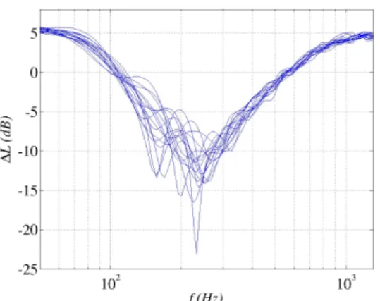
spectrum computed using the same parameters and a configuration with no ground. Figure 4 shows the excess attenuation spectra obtained for all the simulations. The results present a large dispersion. Moreover, from one realization of ground profile to another the sound pressure level may vary strongly. One also can note the additional oscillating behaviour due to the random profiles.
Figure 4: Excess attenuation spectra for 15 simulations with different random ground height profile (zero mean,
sh=0.1m). Hs=Hr=2m, xr=50 m, σ=150 kN.s.m-4.
On Figure 5, the mean value of the fifteen simulations is compared to the excess attenuation spectrum computed for the case of a homogeneous flat ground (σ=150kN.s.m-4).
This mean value has a ground dip lower both in amplitude and frequency, as if the propagation would have been considered above a more absorbing flat ground with a lower air flow resistivity. This result is physically coherent as the ground irregularities induce backscattering of the sound energy.
The uncertainties on the ground profile introduced in the simulations have then an important effect on the sound pressure level (differences up to 10 dB with the homogeneous case).
Figure 5: Mean value and standard deviation of the results of Figure 4 (black and dashed curves) compared to the excess attenuation spectrum in the case of a homogeneous
flat ground (red curve). Hs=Hr=2m, xr=50m,
σ=150kN.s.m-4.
An effective air flow resistivity is estimated for this mean value by fitting an analytical solution of propagation above a flat absorbing ground [12] with the same configuration for the source and the receiver (Figure 6). In this analytical solution, the impedance is also expressed with the Miki model (Eq. (16)). The two curves fit for
σ=85kN.s.m-4 in the analytical solution, while the actual air
flow resistivity of the ground in the simulations is
σ=150kN.s.m-4.
Figure 6: Fitting between the mean value of the computation results (black curve) and an analytical solution
of propagation above a flat ground with Hs=Hr=2m,
This result can be used in the experimental field and applied to the case of ground impedance measurements which consider a perfectly flat ground. As a real ground cannot be regarded as a pure flat ground, a significant underestimation of the air flow resistivity can occur.
5
Effect of ground impedance
uncertainties on SPL
5.1 Simulations
In this section, the effects of ground impedance uncertainties are studied. The configuration is the same as in section 4.1, except for the ground which is perfectly flat.
From impedance measurement campaigns, it is known that experimental uncertainties on the air flow resistivity around 150kN.s.m-4 are about ±20kN.s.m-4 [11]. Fifty
values of σ are drawn with a normal distribution of mean value σ =150kN.s.m-4 and standard deviation
sσ=20kN.s.m-4; they are allocated to 50 one meter long
ground strips along the propagation path as shown on Figure 7.
Figure 7: Example of random air flow resistivity drawing with σ =150 kN.s.m-4 and sσ=20 kN.s.m-4. σ is constant on
each one meter long ground strip.
Coefficients ak and λk are calculated for all of these
values of σ as described in section 3. Fifteen simulations are carried out. For each one the fifty strips are randomly reorganized. Computation time for one simulation is about twenty minutes on four processors.
5.2 Results
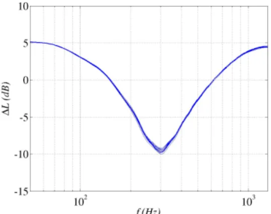
The excess attenuation spectra are obtained for each simulation as described in Section 4.2. They are presented in Figure 8. From one realization of ground impedance to another, the variation of the sound pressure level is very low and there is a small dispersion between the results.
In Figure 9, the mean value of the simulations is compared to the excess attenuation spectrum computed for the case of a homogeneous ground (σ=150kN.s.m-4). The
mean value is very close to the homogeneous case. This shows that the uncertainties on the ground impedance introduced in the simulations do not have a significant influence on the sound pressure level at such distances (50m from the sound source), which agrees with Ostachev’s recent results [5].
Figure 8: Excess attenuation spectra for fifteen simulations with different random ground impedance profile (zero mean, sh=0.1m). Hs=Hr=2m, xr=50m, σ=150kN.s.m-4.
Figure 9: Mean value and standard deviation of the results of Figure 8 (black and dashed curves) compared to the excess attenuation spectrum in the case of a homogeneous
ground (red curve). Hs=Hr=2m, xr=50m, σ=150kN.s.m-4.
6
Conclusion
A first study on the influence of geometrical and ground parameters uncertainties on the prediction of sound levels has been done. The uncertainties values were considered with a range of order issued from the experimental background.
It appears that considering a nearly flat ground by introducing a realistic random ground profile leads to a significant increase of the apparent ground absorption. This result shall be confirmed soon using a curvilinear meshing FDTD code named Code_Safari and developed at EDF R&D which allows the grids to adjust to realistic boundaries.
The sensitivity of the TLM predictions to uncertainties in the air flow resistivity did not reveal any important effect on both the average and the dispersion of the predicted sound pressure levels. In that case the uncertainties were taken at the range of order of experimental uncertainties on a homogeneous ground. A next step could be to consider a bigger dispersion to take into account a realistic space and time variability of the ground properties. This will be tested in further works, especially using the experimental results issued from the Ifsttar Long Term Monitoring Site (LTMS) of Saint-Berthevin [13].
Acknowledgments
This work is currently carried out within the context of a PhD Thesis, partnership between Ifsttar (Nantes, France) and EDF R&D (Clamart, France).
References
[1] O. Baume, “Approche géostatistique de l’influence des paramètres physiques sur la propagation acoustique à grande distance”, PhD Thesis, Université du Maine (2006)
[2] O. Baume, B. Gauvreau, M. Bérengier, F. Junker, H. Wackernagel, J.P. Chilès, “Geostatistical modeling of sound propagation: principles and a field application experiment”, J. Acoust. Soc. Am., Vol. 126(6), 2894– 2904 (2009)
[3] O. Leroy, “Estimation d’incertitudes pour la propagation acoustique en milieu extérieur”, PhD Thesis, Université du Maine (2010)
[4] O. Leroy, B. Gauvreau, F. Junker, E. de Rocquigny, M. Bérengier, “Uncertainty assessment for outdoor sound propagation”, International Congress on Acoustics (ICA) 2010, Sydney (A), 23-27 aug. 2010
[5] V. E. Ostachev, D. K. Wilson, S. N. Vecherin, “Effect of randomly varying impedance on the interference of the direct and ground-reflected waves”, J. Acoust. Soc.
Am. Vol. 130(4), 1844-1850 (2011)
[6] G. Guillaume, “Application de la TLM à la modélisation de la propagation acoustique en milieu urbain”, PhD Thesis, Université du Maine (2009)
[7] P. Aumond, “Modélisation numérique pour l’acoustique environnementale : simulation de champs météorologiques et intégration dans un modèle de propagation”, PhD Thesis, Université du Maine (2011) [8] G. Guillaume, J. Picaut, G. Dutilleux, B. Gauvreau,
“Time-domain impedance formulation for transmission line matrix modeling of outdoor sound propagation”,
Journal of Sound and Vibration 330, 6467-6481 (2011)
[9] J. Hofmann, K. Heutschi, “Simulation of outdoor sound propagation with a transmission line matrix method”, Applied Acoustics 68, 158-172 (2007)
[10] B. Cotté, P. Blanc-Benon, C. Bogey, F. Poisson, “Time-domain impedance boundary conditions for simulations of outdoor sound propagation”, AIAA
Journal 47(10), 2391-2403 (2009)
[11] O. Baume, H. Wackernagel, B. Gauvreau, F. Junker, M. Bérengier “Geostatistical modeling of environmental sound propagation”, GeoENV VI –
Geostatistics for Environmental Applications, 45-57
(2008)
[12] T.F.W. Embleton, J.E. Piercy, G.A. Daigle “Effective flow resistivity of ground surfaces determined by acoustical measurements”, J. Acoust. Soc. Am. 74(4), 1239-1244 (1983)