A Study of NK Landscapes' Basins and Local Optima Networks

HAL Id: hal-00331868

https://hal.archives-ouvertes.fr/hal-00331868

Submitted on 19 Oct 2008

HAL is a multi-disciplinary open access

archive for the deposit and dissemination of

sci-entific research documents, whether they are

pub-lished or not. The documents may come from

teaching and research institutions in France or

abroad, or from public or private research centers.

L’archive ouverte pluridisciplinaire HAL, est

destinée au dépôt et à la diffusion de documents

scientifiques de niveau recherche, publiés ou non,

émanant des établissements d’enseignement et de

recherche français ou étrangers, des laboratoires

publics ou privés.

A Study of NK Landscapes’ Basins and Local Optima

Networks

Gabriela Ochoa, Marco Tomassini, Sébastien Verel, Christian Darabos

To cite this version:

Gabriela Ochoa, Marco Tomassini, Sébastien Verel, Christian Darabos. A Study of NK Landscapes’

Basins and Local Optima Networks. Genetic And Evolutionary Computation Conference, Jul 2008,

Atlanta, United States. pp.555–562, �10.1145/1389095.1389204�. �hal-00331868�

A Study of NK Landscapes’ Basins and

Local Optima Networks

Gabriela Ochoa

Automated Scheduling, Optimisation and Planning School of Computer Science University of Nottingham, UK

gxo@cs.nott.ac.uk

Marco Tomassini

Marco.Tomassini@unil.ch

Seb ´astien V ´erel

Laboratoire I3S CNRS-University of Nice Sophia Antipolis, France

verel@i3s.unice.fr

Christian Darabos

Christian.Darabos@unil.ch

ABSTRACT

We propose a network characterization of combinatorial fitness land-scapes by adapting the notion of inherent networks proposed for

energy surfaces [5]. We use the well-known family ofN K

land-scapes as an example. In our case the inherent network is the graph where the vertices are all the local maxima and edges mean basin adjacency between two maxima. We exhaustively extract such

net-works on representative smallN K landscape instances, and show

that they are ‘small-worlds’. However, the maxima graphs are not random, since their clustering coefficients are much larger than those of corresponding random graphs. Furthermore, the degree distributions are close to exponential instead of Poissonian. We also describe the nature of the basins of attraction and their rela-tionship with the local maxima network.

Categories and Subject Descriptors

I.2.8 [Artificial Intelligence]: Problem Solving, Control Methods, and Search—Heuristic methods; G.2.2 [Discrete Mathematics]: Graph Theory—Network problems

General Terms

Algorithms, Measurement, Performance

Keywords

Landscape Analysis, Network Analysis, Complex Networks, Local

Optima,N K Landscapes

Permission to make digital or hard copies of all or part of this work for personal or classroom use is granted without fee provided that copies are not made or distributed for profit or commercial advantage and that copies bear this notice and the full citation on the first page. To copy otherwise, to republish, to post on servers or to redistribute to lists, requires prior specific permission and/or a fee.

GECCO’08, July 12–16, 2008, Atlanta, Georgia, USA.

Copyright 2008 ACM 978-1-60558-131-6/08/07 ...$5.00.

1.

INTRODUCTION

A fitness landscape of a combinatorial problem can be seen as a graph whose vertices are the possible configurations. If two con-figurations can be transformed into each other by a suitable opera-tor move, then we can trace an edge between them. The resulting graph, with an indication of the fitness at each vertex, is a rep-resentation of the given problem fitness landscape. Doye [5, 6] has recently introduced a useful simplification of the fitness land-scape graph for the energy landland-scapes of atomic clusters. The idea consists in taking as vertices of the graph not all the possible con-figurations, but only those that correspond to energy minima. For atomic clusters these are well-known, at least for relatively small assemblages. Two minima are considered connected, and thus an edge is traced between them, if the energy barrier separating them is sufficiently low. In this case there is a transition state, meaning that the system can jump from one minimum to the other by ther-mal fluctuations going through a saddle point in the energy hyper-surface. The values of these activation energies are mostly known experimentally or can be determined by simulation. In this way, a network can be built which is called the “inherent structure” or “inherent network” in [5]. We use a modification of this idea for

studying the well-known N K combinatorial landscapes. In our

case, a vertex of the graph is a local maximum, and there is an edge between two maxima if they lay on adjacent basins.

In the context of meta-heuristics, it is important to identify the features of landscapes that would influence the effectiveness of heuristic search. Such knowledge may be helpful for both predict-ing the performance and improvpredict-ing the design of meta-heuristics. Among the features of landscapes known to have a strong influence on heuristic search, is the number and distribution of local optima in the search space. An interesting property of combinatorial land-scapes, which has been observed in many different studies, is that on average, local optima are very much closer to the global op-timum than are randomly chosen points, and closer to each other than random points would be. In other words, the local optima are not randomly distributed, rather they tend to be clustered in a ”cen-tral massif” (or “big valley” if we are minimising). This globally

convex landscape structure has been observed in theN K family of

such as the traveling salesman problem [2], graph bipartitioning [13], and flowshop scheduling [16].

In this study we seek to provide fundamental new insights into the structural organization of the local optima in combinatorial land-scapes, particularly into the connectivity and characteristics of their

basins of attraction, using N K landscapes as a case study. To

achieve this, we first map the landscape onto a network, and then

analyze the topology of this network for a number of smallN K

landscape instances for which complete networks can be obtained. Our analysis is inspired, in particular, by the work of Doye [5, 6] on energy landscapes, and in general, by the field of complex net-works [14, 20, 21]. The study of complex netnet-works has already permeated the evolutionary computation field. Specifically, in the study of scientific collaborations [3, 12], the structure of a popu-lation in cellular evolutionary algorithms [9, 10, 15], and the evo-lution of networks of cellular automata [19]. However, our study is the first attempt, to our knowledge, of using network analysis techniques in connection with the study of fitness landscapes and problem difficulty in combinatorial optimization.

The next section introduces the study of complex networks, and describes the main features of small-world and scale-free networks. Section 3 describes how landscapes are mapped onto networks, and includes the relevant definitions and algorithms. The empirical

net-work analysis of our selectedN K landscape instances is presented

in Section 4, whilst Section 5 gives our conclusions and ideas for future work.

2.

COMPLEX NETWORKS

The recent interest in the study of networks and networked sys-tems was influenced by the seminal paper by Watts and Strogatz [21], who showed that many real-world networks are neither com-pletely ordered nor comcom-pletely random, but rather exhibit important properties of both. Some of these network properties can be

quanti-fied by simple statistics such as the clustering coefficientC, which

is a measure of local density, and the average shortest path length

l, which is a global measure of separation. It has been shown in

re-cent years that many social, biological, and man-made system show what has been called a small-world topology [21], in which nodes are highly clustered yet the path length between them is small.

A second important aspect in the study of networks has been the realization that in many real-world networks, the distribution of the number of neighbours (the degree distribution) is typically right-skewed with a ”heavy tail”, meaning that most of the nodes have less-than-average degree whilst a small fractions of hubs have a large number of connections. These qualitative description can be described mathematically by a power-law [1], which has the

asymptotic formp(k) ∼ k−α_{. This means that the probability of}

a randomly chosen point having a degreek decays like a power of

k, where the exponent α (typically in the range [2, 3]) determines

the rate of decay. A distinguishing feature of power-law distribu-tions is that when plotted on a double logarithmic scale, a

power-law appears as a straight line with negative slopeα. This

behav-ior contrasts with a normal distribution which would curve sharply on a log-log plot, such that the probability of a node having a de-gree greater than a certain ”cutoff” value is nearly zero. The mean would then trivially represent a characteristic scale for the network degree distribution. Since networks with power-low degree distri-bution lack any such cutoff value, at least in theory, they are often called scale-free networks [20]. Examples of such scale-free net-works are the world-wide-web, the internet, scientific collaboration and citation networks, and biochemical networks.

3.

LANDSCAPES AS NETWORKS

To model a physical energy landscape as a network, Doye [6] needed to decide first on a definition both of a state of the system and how two states were connected. The states and their connec-tions will then provide the nodes and edges of the network. For sys-tems with continuous degrees of freedom, the author achieved this through the ‘inherent structure’ mapping [18]. In this mapping each point in configuration space is associated with the minimum (or ‘inherent structure’) reached by following a steepest-descent path from that point. This mapping divides configuration into basins of attraction surrounding each minimum on the energy landscape.

We use a modification of this idea for the N K family of

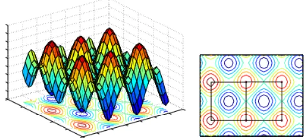
bi-nary landscapes, which indeed can be applied to any combinato-rial landscape. In our case, the vertexes of the graph are the local maxima of the landscape, obtained exhaustively by running a best-improvement local search algorithm (see Algorithm 1) from every configuration of the search space. The edges in the network connect local optima of adjacent basins of attraction. An illustration for a model 2D landscape can be seen in Figure 1, which is inspired by a similar figure appearing in [5, 6]. Here, we illustrate a network of local maxima (instead of local minima). A more formal definition of our inherent networks is given in Section 3.1. As it was the case in the study on physical energy landscapes [6], we do not consider multiple edges, or weights in the edges. This may be a factor to consider in future work.

Figure 1: A model of a 2D landscape (left), and a contour plot of the local optima partition of the configuration space into basins of attraction surrounding maxima and minima (right). A sim-ple regular network of six local maxima can be observed.

Note that while a physical energy landscape is formally a con-tinuous landscape, ours are strictly combinatorial, i.e. discrete and finite. Moreover, the energy landscape of a stable atomic cluster, crystal or molecule is relatively smooth and easy to search and has

been called a “funnel” landscape [5]. In contrast, inN K

land-scapes one can continuously vary the intrinsic landscape difficulty

by changing the value ofK. As a result, we shall see that N K

landscapes show a number of different behaviors depending onK

for a givenN , and these different behaviors are reflected on their

inherent networks. Indeed,N K landscapes can be seen as

analo-gous to those of spin-glasses [11, 17]. In contrast to atomic cluster energy landscapes, spin glass landscapes may show frustration, i.e. configurations that must respect conflicting constraints, and solving for the ground state of the system that is, the minimum energy con-figuration is an NP-hard problem. Similar consequences are caused by the introduction of epistatic interactions through the increase of theK value in N K landscapes.

Below we present the relevant formal definitions and algorithms to obtain our combinatorial analogous of an energy landscape in-herent network.

3.1

Definitions and Algorithms

Definition : Fitness landscape.

A landscape is a triplet(S, V, f ) where S is a set of potential

solu-tions i.e. a search space,V : S −→ 2S, a neighborhood structure,

is a function that assigns to everys ∈ S a set of neighbours V (s),

andf : S −→ R is a fitness function that can be pictured as the

height of the corresponding potential solutions.

In our study, the search space is composed by binary strings of

lengthN , therefore its size is 2N_{. The neighborhood is defined by}

the minimum possible move on a binary search space, that is, the 1-move or bit-flip operation. In consequence, for any given string

s of length N , the neighborhood size is |V (s)| = N . Notice that

inN K landscapes, two neighboring solutions never have the same

fitness value. Therefore, neutrality is not present. Landscapes with neutrality will be considered in future work.

Definition: Local Optimum.

A local optimum is a solutions∗

such that∀s ∈ V (s∗

), f (s) < f (s∗

).

TheLocalSearch algorithm to determine the local optima and

therefore define the basins of attraction, is given below:

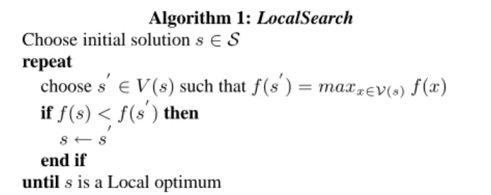
Algorithm 1: LocalSearch

Choose initial solutions ∈ S

repeat

chooses′∈ V (s) such that f (s′) = maxx∈V(s)f (x)

iff (s) < f (s′) then s ← s′

end if

untils is a Local optimum

TheLocalSearch algorithm defines a mapping from the search

spaceS to the set of locally optimal solutions S∗

. We therefore define a basin of attraction as follows:

Definition : Basin of attraction.

The basin of attraction of a local optimumi is the set bi = {s ∈

S | LocalSearch(s) = i}. The size of the basin of attraction of a

local optimai is the cardinality of bi.

We then define the inherent network, or network of local optima as:

Definition : Local optima network.

The local optima networkG = (S∗

, E) is the graph where the

nodes are the local optima, and there is an edgeeij ∈ E between

two local optimai and j if there is at least a pair of direct neighbors

(1-bit apart)siandsj, such thatsi ∈ biandsj ∈ bj. That is, if

there exists a pair of direct neighbors solutionssi andsj, one in

each basin (biandbj)

4.

EMPIRICAL NETWORK ANALYSIS

4.1

Experimental Setting

TheN K family of landscapes [11] is a problem-independent

model for constructing multimodal landscapes that can gradually

be tuned from smooth to rugged. In the model,N refers to the

number of (binary) genes in the genotype (i.e. the string length) andK to the number of genes that influence a particular gene. By

increasing the value ofK from 0 to N − 1, N K landscapes can be

tuned from smooth to rugged. Thek variables that form the context

of the fitness contribution of genesican be chosen according to

dif-ferent models. The two most widely studied models are the random

neighborhood model, where thek variables are chosen randomly

according to a uniform distribution among then − 1 variables other

thansi, and the adjacent neighborhood model, in which thek

vari-ables that are closest tosi in a total orderings1, s2, . . . , sn

(us-ing periodic boundaries). No significant differences between the two models were found in [11] in terms of global properties of the respective families of landscapes, such as mean number of local optima or autocorrelation length. Therefore, we explore here the adjacent neighborhood model, leaving the random model for future analysis.

In order to avoid sampling problems that could bias the results,

we used the largest values ofN that can still be analyzed

exhaus-tively with reasonable computational resources. We thus extracted

the local optima networks of landscape instances withN = 16, 18,

andK = 2, 4, 6, ..., N − 2, N − 1. For each pair of N and K

val-ues, 30 instances were explored. Therefore, the networks statistics reported below represent the average behaviour of 30 independent instances.

4.2

General Network Statistics

Table 1 reports the average of the network properties measured onN K landscapes for N = 16, 18 and all even K values; K = N − 1 is also given. Values are averages over 30 randomly

gener-ated landscapes. n¯vandn¯eare, respectively, the mean number of

vertices and the mean number of edges of the graph for a givenK

rounded to the next integer. ¯C is the average of the mean clustering

coefficients1_{over all the generated landscapes. C}

r is the average

clustering coefficient of a random graph with the same number of

vertices and mean degree.¯z is the average of the mean degrees. ¯l is

the average of the mean path lengths over all landscape instances. The last column contains the average degree assortativity

coeffi-cient¯a, which measures whether nodes with similar degrees tend

to pair up with each other. The assortativity coefficient is computed according to [14].

Notice that the mean number of vertexes (n¯v) confirms that the

number of local optima (and thus the search difficulty) increases

with the value of K. Some other interesting inferences can be

drawn from these metrics. First of all, looking at the ¯l values one

can conclude that the maxima networks are small worlds for all

val-ues ofK since the growth of ¯l is bounded by a function O(log nv).

In a sense, this is not surprising as the whole configuration space

spans the binary hypercube{0, 1}N_{of degreeN with 2}N_vertices,

which has maximum distance (diameter)d = log2N, i.e. 16 and

18 for our studied instances. However, while the base configuration space has constant degree for any node, the maxima network are degree-inhomogeneous (see next section) and have clustering co-efficients well above those of equivalent random graphs, showing

that there is local structure in the networks. For bothN = 16 and

18, the mean degreez first increases with K and then goes down¯

again for K > 8. The assortativity coefficients are always very

small which means that there is almost no correlation between the degrees of neighboring nodes. For easy energy landscapes, Doye found that the networks were slightly disassortative [6].

4.3

Degree Distributions

The degree distribution functionp(k) of a graph represents the

probability that a randomly chosen node has degreek [14].

Ran-dom graphs are characterized by ap(k) of Poissonian form, while

1

The clustering coefficient Ci of a node i is defined as Ci =

2Ei/ki(ki− 1), where Ei is the number of edges in the

neigh-borhood ofi. Thus Cimeasures the amount of “cliquishness” of

the neighborhood of nodei and it characterizes the extent to which

nodes adjacent to nodei are connected to each other. The

cluster-ing coefficient of the graph is simply the average over all nodes:

C = 1 N

PN

Table 1: Network properties ofN K landscapes for N = 16, 18 and all even K values; K = N − 1 is also given. Values are averages over 30 randomly generated landscapes, standard deviations are shown as subscripts.nvandnerepresent the number of vertexes

and edges (rounded to the next integer), ¯C, the mean clustering coefficient, whilst Cris the clustering coefficient of a random graph

with the same number of vertexes and mean degree, which isCr≃ ¯z/¯nv.z represent the mean degree, ¯¯ l the mean path length , and

¯

a the degree assortativity coefficient.

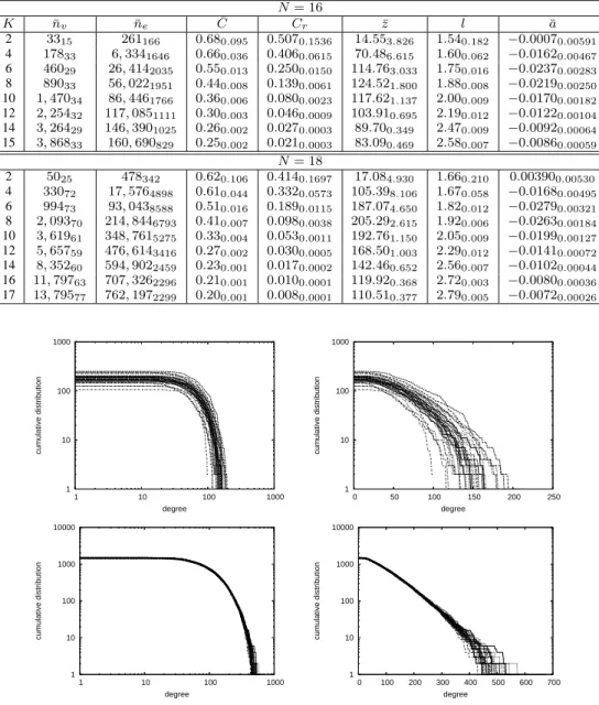
N = 16 K n¯v n¯e C¯ Cr z¯ ¯l ¯a 2 33₁₅ 261₁₆₆ 0.680.095 0.5070.1536 14.553.826 1.540.182 −0.00070.00591 4 178₃₃ 6_{, 3341646} 0_.660.036 0_.4060.0615 70_.486.615 1_{.600.062 −}0_.01620.00467 6 460₂₉ 26_{, 4142035} 0_.550.013 0_.2500.0150 114_.763.033 1_{.750.016 −}0_.02370.00283 8 890₃₃ 56_{, 0221951} 0_.440.008 0_.1390.0061 124_.521.800 1_{.880.008 −}0_.02190.00250 10 1_{, 47034} 86_{, 4461766} 0_.360.006 0_.0800.0023 117_.621.137 2_{.000.009 −}0_.01700.00182 12 2_{, 25432} 117_{, 0851111} 0_.300.003 0_.0460.0009 103_.910.695 2_{.190.012 −}0_.01220.00104 14 3_{, 26429} 146_{, 3901025} 0_.260.002 0_.0270.0003 89_.700.349 2_{.470.009 −}0_.00920.00064 15 3, 86833 160, 690829 0.250.002 0.0210.0003 83.090.469 2.580.007 −0.00860.00059 N = 18 2 50₂₅ 478₃₄₂ 0.620.106 0.4140.1697 17.084.930 1.660.210 0.003900.00530 4 330₇₂ 17_{, 5764898} 0_.610.044 0_.3320.0573 105_.398.106 1_{.670.058 −}0_.01680.00495 6 994₇₃ 93, 0438588 0.510.016 0.1890.0115 187.074.650 1.820.012 −0.02790.00321 8 2_{, 09370} 214_{, 8446793} 0_.410.007 0_.0980.0038 205_.292.615 1_{.920.006 −}0_.02630.00184 10 3_{, 61961} 348_{, 7615275} 0_.330.004 0_.0530.0011 192_.761.150 2_{.050.009 −}0_.01990.00127 12 5_{, 65759} 476_{, 6143416} 0_.270.002 0_.0300.0005 168_.501.003 2_{.290.012 −}0_.01410.00072 14 8_{, 35260} 594_{, 9022459} 0_.230.001 0_.0170.0002 142_.460.652 2_{.560.007 −}0_.01020.00044 16 11, 79763 707, 3262296 0.210.001 0.0100.0001 119.920.368 2.720.003 −0.00800.00036 17 13_{, 79577} 762_{, 1972299} 0_.200.001 0_.0080.0001 110_.510.377 2_{.790.005 −}0_.00720.00026 1 10 100 1000 1 10 100 1000 cumulative distribution degree 1 10 100 1000 0 50 100 150 200 250 cumulative distribution degree 1 10 100 1000 10000 1 10 100 1000 cumulative distribution degree 1 10 100 1000 10000 0 100 200 300 400 500 600 700 cumulative distribution degree

Figure 2: Cumulative degree distributions forN = 16 and K = 4 (top), K = 10 (bottom). All 30 curves are plotted. Left: Log-log plot. Right: Lin-log plot.

social and technological real networks often show long tails to the right, i.e. there are nodes that have an unusually large number of neighbors. Sometimes this behavior can be described by a power-law, but often the distribution is less extreme and can be fitted by a stretched exponential or by an exponentially truncated power-law[14].

Figure 2 shows all the curves for 30 randomly generated

land-scapes forN = 16 and K = 4, 10, whilst figure 3 does the same

forN = 18. To smooth out fluctuations in the high degree region,

the cumulative degree distribution function is plotted, which is just

the probability that the degree is greater than or equal tok. The

sin-gle curves are shown rather than the average curve because the sum of a sufficient number of independent random variables with arbi-trary distributions, provided that the first few moments exist and are finite, tends to distribute normally according to a general formula-tion of the central limit theorem [7]. In other words, if the average of the sum were plotted, the original shapes would essentially be lost. The curves cannot be described by power-laws: this possibil-ity is ruled out by the left parts of figs. 2, and 3 which are double logarithmic plots. In log-log plots, power laws should appear as straight lines, at least for a sizable part of abscissae range.

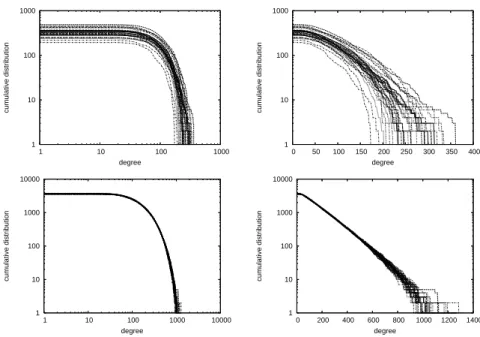
1 10 100 1000 1 10 100 1000 cumulative distribution degree 1 10 100 1000 0 50 100 150 200 250 300 350 400 cumulative distribution degree 1 10 100 1000 10000 1 10 100 1000 10000 cumulative distribution degree 1 10 100 1000 10000 0 200 400 600 800 1000 1200 1400 cumulative distribution degree

Figure 3: Cumulative degree distributions forN = 18 and K = 4 (top), K = 10 (bottom). All 30 curves are plotted. Left: Log-log plot. Right: Lin-log plot.

the distributions can be fitted approximately by exponentials of the typep(k) = (1/z)e−k/z _{wherez is the mean degree, as most}

curves are approximately straight lines on these linear-log plots. This is true for the larger part of the degree range. When we ap-proach the finite degree cutoff the fit is obviously less good. Small

networks such as those withN = 16 and K = 4 show larger

fluctuations and their tails decay faster than exponentially. Two

particular examples with a medium value ofK (K = 8) are shown

in detail in fig. 4, together with an exponential fit. Table 2 gives the

parameters of the regression lines for allN and K values.

Table 2: Correlation coefficient (ρ), intercept ( ¯¯ α) and slope ( ¯β) and slope of the linear regression between the cumulative num-ber of nodes and the degree of nodes :log(p(k)) = α + βk + ǫ. The averages and standard deviations of 30 independent land-scapes, are shown.

N = 16 K _ρ¯ _α¯ _β¯ 2 −0.8160.340 4.050.717 −0.11090.0379 4 −0.9320.026 6.070.276 −0.02950.0026 6 −0.9670.009 7.090.105 −0.01780.0009 8 −0.9860.006 7.600.107 −0.01440.0007 10 −0.9890.004 8.040.125 −0.01460.0008 12 −0.9900.004 8.510.156 −0.01700.0010 14 −0.9920.003 8.920.121 −0.02020.0010 15 −0.9910.004 9.110.144 −0.02200.0011 N = 18 2 −0.8230.343 4.570.865 −0.10880.0325 4 −0.9510.025 6.710.225 −0.01980.0021 6 −0.9820.007 7.740.107 −0.00980.0005 8 −0.9910.004 8.280.096 −0.00760.0003 10 −0.9940.003 8.740.119 −0.00760.0004 12 −0.9950.003 9.190.161 −0.00880.0005 14 −0.9950.003 9.650.134 −0.01100.0005 16 −0.9940.003 10.10.173 −0.01390.0008 17 −0.9940.005 10.20.207 −0.01510.0008 1 10 100 1000 10000 0 100 200 300 400 500 600 cumulative distribution degree exp. regr. line 1 10 100 1000 10000 0 100 200 300 400 500 600 700 800 900 1000 cumulative distribution degree exp. regr. line

Figure 4: Cumulative degree distribution (with regression line) of two representative instances withK = 8, N = 16 (top) and N = 18 (bottom).

If we compare these results with Doye’s [5, 6] the most impor-tant difference is that we do not observe power-law distributions. Indeed, power-law degree distributions of the inherent energy land-scape networks point to the “easiness” of those landland-scapes: due to the presence of highly connected nodes, which are also among the fittest, a simple gradient-descent would bring a searcher down to a local energy minimum, often the global one, starting anywhere in the configuration space. In other words, there exist the “funnel”

effect described by Doye [5]. In contrast,N K landscapes have

tunable difficulty. How can random networks with exponential de-gree distributions be obtained? One way is the following: in each time step, just add a new node, and add a new link between two randomly chosen nodes, including the new one. Iterating this dy-namical process produces graphs with an exponential distribution

of the node degrees [4]. ButN K landscapes are static and thus it is

difficult to see how this process could be implemented. However,

the following qualitative explanation might help. Imagine thatK is

increased from 2 toN − 1 in single steps. Then we could have the

image of the previous landscape increasing its size and deforming

itself whenK goes from its current value to K + 1. The new

max-ima that appear could be considered as if they were added dynam-ically (of course some previous optima might disappear as well). Edges in the new landscape are selected essentially randomly, with more probability of selecting an already existing node. Thus, with this imaginary mechanism a distribution close to exponential would be obtained.

Thus, as theN K landscape difficulty varies smoothly when K

is increased, the degree distribution of the corresponding maxima networks remains essentially exponential. We do not observe scale-free distributions for the easy landscapes as in the energy landscape case [5]. This is understandable: standard energy landscapes in molecular chemistry and crystal physics do correspond to thermo-dynamically stable states which are naturally smooth and easy to reach when the system is forming or it is slightly perturbed. In

contrast,N K landscape are synthetic and do not correspond to any

physical principle in their construction. The only physical systems

that resembleN K landscapes are spin glasses, in which conflicting

energy minimization requirements lead to frustration and to land-scape ruggedness [11, 17]. However, disordered condensed matter systems similar to spin glasses are only obtained in particular situ-ations, for instance by fast cooling [17].

4.4

Basins of Attraction

Besides the maxima network, it is useful to describe the asso-ciated basins of attraction as these play a key role in search al-gorithms. Furthermore, some characteristics of the basins can be related to the network features described above. The notion of the basin of attraction of a local maximum has been presented in sect. 3.1. We have exhaustively computed the size and number of

all the basins of attraction forN = 16 and N = 18 and for all even

K values plus K = N − 1. In this section, we analyze the basins

of attraction from several points of view as it is described below.

4.4.1

Global optimum basin size vs.

In Figure 5 we plot the average size of the basin corresponding

to the global maximum forN = 16 and N = 18, and all values

ofK studied. The trend is clear: the basin shrinks very quickly

with increasingK. This confirms that the higher the K value, the

more difficult for an stochastic search algorithm to locate the basin of attraction of the global optimum

4.4.2

Number of basins of a given size

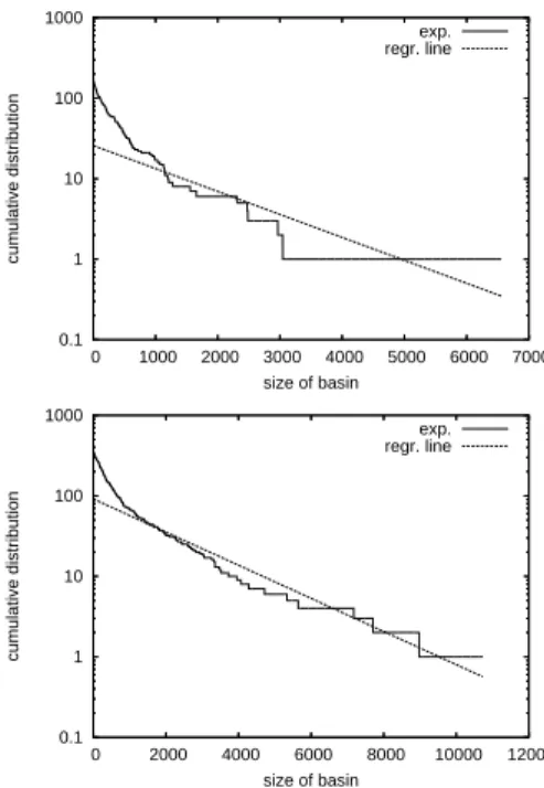
Figure 6 shows the cumulative distribution of the number of basins of a given size (with regression line) for two representative

instances withK = 4 and N = 16 (top) and N = 18. Table 3

shows the average (of 30 independent landscapes) correlation

co-efficients and linear regression coco-efficients (intercept (α) and slope¯

( ¯β)) between the number of nodes and the basin sizes. Notice that

distribution decays exponentially or faster for the lowerK and it

is closer to exponential for the higherK. This observation is

rele-vant to theoretical studies that estimate the size of attraction basins

1e-04 0.001 0.01 0.1 1 2 4 6 8 10 12 14 16 18

relative size of the global optima’s basin

K

N=16 N=18

Figure 5: Average of the relative size of the basin corresponding to the global maximum for each K over 30 landscapes.

0.1 1 10 100 1000 0 1000 2000 3000 4000 5000 6000 7000 cumulative distribution size of basin exp. regr. line 0.1 1 10 100 1000 0 2000 4000 6000 8000 10000 12000 cumulative distribution size of basin exp. regr. line

Figure 6: Cumulative distribution of the number of basins of a given size with regression line. Two Representative landscapes are visualized with N=16 (top) and N=18 (bottom) and K=4. A lin-log scale is used.

(see for example [8]). These studies often assume that the basin

sizes are uniformly distributed. From the slopes ¯β of the regression

lines (table 3) one can see that high values ofK give rise to steeper

distributions (higher ¯β values). This indicates that there are less

basins of large size for large values ofK. In consequence, basins

are broader for low values ofK, which is consistent with the fact

that those landscapes are smoother.

4.4.3

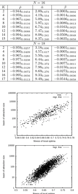
Fitness of local optima vs. their basin sizes

The scatter-plots in figure 7 illustrate the correlation between the basin sizes of local maxima (in logarithmic scale) and their fitness

values. Two representative instances forN = 18 and K = 4,8 are

shown. Table 4 shows the averages (of 30 independent landscapes) of the correlation coefficient, and the linear regression coefficients

Table 3: Correlation coefficient (ρ), and linear regression co-¯ efficients (intercept (α) and slope ( ¯¯ β)) of the relationship be-tween the basin size of optima and the cumulative number of nodes of a given (basin) size ( in logarithmic scale:log(p(s)) = α + βs + ǫ). The average and standard deviation values over 30 instances, are shown.

N = 16 K ρ¯ α¯ β¯ 2 −0.9440.0454 2.890.673 −0.00030.0002 4 −0.9590.0310 4.190.554 −0.00140.0006 6 −0.9670.0280 5.090.504 −0.00360.0010 8 −0.9820.0116 5.970.321 −0.00800.0013 10 −0.9850.0161 6.740.392 −0.01630.0025 12 −0.9900.0088 7.470.346 −0.03040.0042 14 −0.9940.0059 8.080.241 −0.05080.0048 15 −0.9950.0044 8.370.240 −0.06350.0058 N = 18 2 −0.9590.0257 3.180.696 −0.00010.0001 4 −0.9600.0409 4.570.617 −0.00050.0002 6 −0.9670.0283 5.500.520 −0.00150.0004 8 −0.9770.0238 6.440.485 −0.00370.0007 10 −0.9850.0141 7.240.372 −0.00770.0011 12 −0.9890.0129 7.980.370 −0.01500.0019 14 −0.9930.0072 8.690.276 −0.02720.0024 16 −0.9950.0056 9.330.249 −0.04500.0036 17 −0.9920.0113 9.490.386 −0.05440.0058 1 10 100 1000 10000 100000 0.56 0.58 0.6 0.62 0.64 0.66 0.68 0.7 0.72 0.74 0.76 0.78

basin of attraction size

fitness of local optima exp. regr. line 1 10 100 1000 10000 0.5 0.55 0.6 0.65 0.7 0.75 0.8

basin of attraction size

fitness of local optima regr. line

Figure 7: Correlation between the fitness of local optima and their corresponding basin sizes, for two representative in-stances withN = 18, K = 4 (top) and K = 8 (bottom).

between these two metrics (maxima fitness and their basin sizes).

All the studied landscapes forN = 16 and 18, are reported. Notice

that, there is a clear positive correlation between the fitness values of maxima and their basins’ sizes. In other words, the higher the peak the wider tend to be its basin of attraction. Therefore, on average, with a hill-climbing algorithm, the global optimum would be easier to find than any other local optimum. This may seem

Table 4: Correlation coefficient (ρ), and linear regression coef-¯ ficients (intercept (α) and slope ( ¯¯ β)) of the relationship between the fitness of optima and their basin size (in logarithmic scale: log(s) = α + βf + ǫ). The average and standard deviation values over 30 instances, are shown

N = 16 K ρ¯ α¯ _β¯ 2 0.8320.0879 −15.4765.9401 33.0668.9252 4 0_{.8420.0259 −}13_.0351.9907 27_.0942.8611 6 0.8520.0180 −12.9770.9921 26.0611.4908 8 0_{.8600.0088 −}12_.5700.3769 24_.8800.5725 10 0.8500.0050 −11.9540.3501 23.5610.5421 12 0_{.8330.0065 −}11_.4850.2993 22_.5190.4773 14 0.8160.0047 −11.2610.2008 21.8640.3256 15 0_{.8120.0044 −}11_.3520.2109 21_.8760.3298 N = 18 2 0.8390.0680 −16.5856.0606 35.9258.6640 4 0_{.8420.0257 −}14_.4582.1746 30_.1743.1520 6 0.8520.0140 −14.5420.9596 29.2191.4147 8 0_{.8670.0066 −}14_.5150.3750 28_.5380.5988 10 0.8660.0038 −13.9140.3068 27.2090.4621 12 0_{.8540.0030 −}13_.1800.1700 25_.7510.2804 14 0.8360.0027 −12.6020.1399 24.5530.2214 16 0.8220.0022 −12.5020.1039 24.1330.1633 17 0_{.8170.0027 −}12_.5830.1278 24_.1430.2066

surprising. But, we have to keep in mind that as the number of local

optima increases (with increasing K), the global optimum basin

is more difficult to reach by an stochastic local search algorithm

(see figure 5). This observation offers a mental picture of N K

landscapes: we can consider the landscape as composed of a large number of mountains (each corresponding to a basin of attraction), and those mountains are wider the taller the hilltops. Moreover, the size of a mountain basin grows exponentially with its hight.

4.4.4

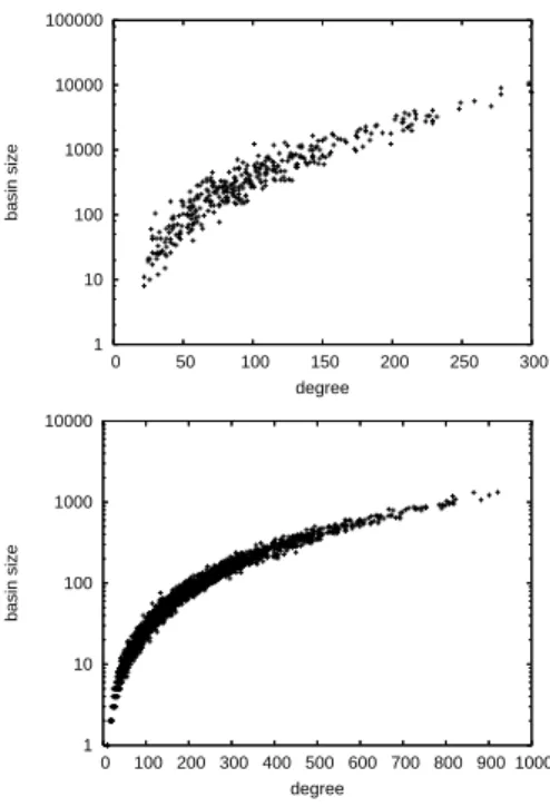
Basins sizes of local optima vs. their degrees

The scatter plots in figure 8 illustrate the correlation between basin sizes of maxima and their degrees. Representative instances withN = 18, and K = 4, 8, are illustrated. There is a clear

pos-itive correlation between the degree and the basin sizes of maxima in the network. This observation suggests that landscapes with low

K values can be searched more effectively since a given

config-uration has many neighbors belonging to the same large basin of

attraction. It is also confirmed that the basins for lowK are much

larger than those for highK, not only the basin corresponding to

the global maximum.

5.

CONCLUSIONS

We have proposed a new characterization of combinatorial

fit-ness landscapes using the well-known family ofN K landscapes as

an example. We have used an extension of the concept of inher-ent networks proposed for energy surfaces [5] in order to abstract and simplify the landscape description. In our case the inherent network is the graph where the vertices are all the local maxima and edges mean basin adjacency between two maxima. We have

exhaustively obtained these graphs forN = 16 and N = 18, and

for all even values ofK, plus K = N − 1. The maxima graphs

are small worlds since the average path lengths are short and scale logarithmically in the size of the graphs. However, the maxima graphs are not random. This is shown by their clustering coeffi-cients, which are much larger than those of corresponding random graphs and also by their degree distribution functions, which are not

1 10 100 1000 10000 100000 0 50 100 150 200 250 300 basin size degree 1 10 100 1000 10000 0 100 200 300 400 500 600 700 800 900 1000 basin size degree

Figure 8: Correlation between the degree of local optima and their corresponding basin sizes, for two representative in-stances with withN = 18, K = 4 (top) and K = 8 (bottom).

Poissonian but rather exponential. The construction of the maxima networks requires the determination of the basins of attraction of the corresponding landscapes. We have thus described the nature of the basins and their relationship with the local maxima network. We have found that the size of the basin corresponding to the global

maximum becomes smaller with increasingK. The distribution of

the basin sizes is approximately exponential for allN and K, but

the basin sizes are larger for lowK, another indirect indication of

the increasing randomness and difficulty of the landscapes when

K becomes large. Finally, there is a strong positive correlation

be-tween the basin size of a maxima and their degree, which confirms that the synthetic view provided by the maxima graph is a useful one.

This study represents our first attempt towards a topological and statistical characterization of easy and hard combinatorial land-scapes. Much remains to be done. First of all, the results found

should be confirmed for larger instances ofN K landscapes. This

will require good sampling techniques, or theoretical studies since exhaustive sampling becomes quickly impractical. Other landscape types should also be examined, such as those containing neutral-ity, which are very common in real-world applications. Work is in

progress for neutral versions ofN K landscapes. Finally, the

land-scape statistical characterization is only a step toward implement-ing good methods for searchimplement-ing it. We thus hope that our results will help in designing or estimating efficient search techniques and operators.

6.

ADDITIONAL AUTHORS

7.

REFERENCES

[1] A-L. Barabasi and R. Albert, Emergence of scaling in

random networks, Science 286 (1999), 509–512.

[2] K. D. Boese, A. B. Kahng, and S. Muddu, A new adaptive

multi-start technique for combinatorial global optimizations,

Operations Research Letters 16 (1994), 101–113.

[3] C. Cotta and J.-J. Merelo, Where is evolutionary computation

going? A temporal analysis of the EC community, Genetic

Programming and Evolvable Machines 8 (2007), 239–253. [4] S. N. Dorogovtsev and J. F. F. Mendes, Evolution of

networks, Oxford University Press, Oxford, New York, 2003.

[5] J. P. K. Doye, The network topology of a potential energy

landscape: a static scale-free network, Phys. Rev. Lett. 88

(2002), 238701.

[6] J. P. K. Doye and C. P. Massen, Characterizing the network

topology of the energy landscapes of atomic clusters, J.

Chem. Phys. 122 (2005), 084105.

[7] W. Feller, An introduction to probability theory and its

applications, Wiley, New York, 1968.

[8] J. Garnier and L. Kallel, Efficiency of local search with

multiple local optima, SIAM Journal on Discrete

Mathematics 15 (2001), no. 1, 122–141.

[9] M. Giacobini, M. Preuss, and M. Tomassini, Effects of

scale-free and small-world topologies on binary coded self-adaptive CEA, Evolutionary Computation in

Combinatorial Optimization – EvoCOP 2006 (Budapest), LNCS, vol. 3906, Springer Verlag, 2006, pp. 85–96. [10] M. Giacobini, M. Tomassini, and A. Tettamanzi, Takeover

time curves in random and small-world structured populations, Genetic and Evolutionary Computation

Conference, GECCO 2005, Proceedings, ACM, 2005, pp. 1333–1340.

[11] S. A. Kauffman, The origins of order, Oxford University Press, New York, 1993.

[12] L.Luthi, M. Tomassini, M. Giacobini, and W. B. Langdon,

The genetic programming collaboration network and its communities, Genetic and Evolutionary Computation

Conference, GECCO 2007, Proceedings, London, England, UK (Hod Lipson et al., ed.), ACM, 2007, pp. 1643–1650. [13] P. Merz and B. Freisleben, Memetic algorithms and the

fitness landscape of the graph bi-partitioning problem,

Parallel Problem Solving from Nature V (A. E. Eiben, T. B¨ack, M. Schoenauer, and H.-P. Schwefel, eds.), Lecture Notes in Computer Science, vol. 1498, Springer-Verlag, 1998, pp. 765–774.

[14] M. E. J. Newman, The structure and function of complex

networks, SIAM Review 45 (2003), 167–256.

[15] J. L. Payne and M. J. Epstein, Takeover times on scale-free

topologies, Genetic and Evolutionary Computation

Conference, GECCO 2007, Proceedings, London, England, UK (Hod Lipson et al., ed.), ACM, 2007, pp. 308–315. [16] C. R. Reeves, Landscapes, operators and heuristic search,

Annals of Operations Research 86 (1999), 473–490. [17] D. L. Stein, Disordered sytems: mostly spin glasses, Lectures

in the Sciences of Complexity (D. L. Stein, ed.), Addison-Wesley, 1989, pp. 301–353.

[18] F.H. Stillinger, A topographic view of supercooled liquids

and glass formation, Science 267 (1995), 1935–1939.

[19] M. Tomassini, M. Giacobini, and C. Darabos, Evolution of

small-world networks of automata for computation, Parallel

Problem Solving from Nature - PPSN VIII (Birmingham, UK), LNCS, vol. 3242, Springer-Verlag, 2004, pp. 672–681. [20] D. J. Watts, The ”new” science of networks, Annual Review

[21] D. J. Watts and S. H. Strogatz, Collective dynamics of