HAL Id: cea-02924467
https://hal-cea.archives-ouvertes.fr/cea-02924467
Submitted on 28 Aug 2020HAL is a multi-disciplinary open access archive for the deposit and dissemination of sci-entific research documents, whether they are pub-lished or not. The documents may come from teaching and research institutions in France or abroad, or from public or private research centers.
L’archive ouverte pluridisciplinaire HAL, est destinée au dépôt et à la diffusion de documents scientifiques de niveau recherche, publiés ou non, émanant des établissements d’enseignement et de recherche français ou étrangers, des laboratoires publics ou privés.
A GEOMETRICAL APPROACH TO EVALUATING
THE HEAT FLUX PEAKING FACTOR ON FIRST
WALL COMPONENTS
R. Mitteau, P. Stangeby
To cite this version:
R. Mitteau, P. Stangeby. A GEOMETRICAL APPROACH TO EVALUATING THE HEAT FLUX PEAKING FACTOR ON FIRST WALL COMPONENTS. Journal of Nuclear Materials, Elsevier, 2009, pp.1022 - 1025. �10.1016/j.jnucmat.2009.01.270�. �cea-02924467�
Journal of Nuclear Materials, Volumes 390–391, 2009, Pages 1022-1025 ISSN 0022-3115
https://doi.org/10.1016/j.jnucmat.2009.01.270
http://www.sciencedirect.com/science/article/pii/S0022311509002888
This is a postprint (see https://en.wikipedia.org/wiki/Postprint), prepared after peer review and publication. The technical content is identical to the published paper, reference 12 has been updated to match the final real publication reference.
A GEOMETRICAL APPROACH TO EVALUATING THE HEAT FLUX
PEAKING FACTOR ON FIRST WALL COMPONENTS
R. Mitteau1*, and P. Stangeby2
1 Association Euratom - CEA sur la Fusion Contrôlée, direction des sciences de la matière,
Centre d'Etude de Cadarache F-13108 Saint Paul Lez Durances CEDEX
2 General Atomics , San Diego, California 92186-5608, US, and University of Toronto
Institute for Aerospace Studies, 4925 Dufferin St., Toronto, M3H 5T6, Canada.
Abstract
In magnetic fusion experiments, a simple technique to evaluate the heat flux on first wall
components is a key to controlled plasma surface interaction. The heat flux can be
characterized by the peaking factor which is the ratio of the peak heat flux to the average heat
flux. The peaking factor can be calculated exactly using simple derivations and standard
software tools. This analysis is applied to an Iter class experiment for plasma wall contact
during start up phases at 15 MW, in idealised, realistic and misaligned situations. Even
though the peaking factors are usually above 10, the peak heat load on the wall remains
moderate at a few MW/m².
1.
Introduction
Estimating the peak heat load (qmax) on plasma facing components (PFCs) before plasma
operation is a key safety issue of plasma surface interaction analysis. Various methods are
possible and can be categorised according to their principles. More scientific techniques start
from the plasma characteristics (temperature, density, transport, sheath transmission
coefficient) and then express the heat flux to the component. These methods are often limited
by the imprecision of the plasma characteristics and especially the transport coefficients. The
most elaborated derivations make use of edge plasma codes, assuring a high level of self
consistence [1-3]. Accounting for the detailed wall connections eventually requires a 3D
mapping of the SOL [4], allowing a rather comprehensive description of small scale plasma
variations. A completely different technique uses the monte carlo principle [5] but is of little
practical use as it requires extensive calculation time for actual 3D wall surfaces. Other
authors have used semi-analytic derivations [6,7] which are dependant on the experiment and
only allow an approximate accounting of the cross component shadow. The most elementary
method consists in dividing the exhaust power (Ptotal) by the component area (A), which gives
an average heat load (qmean = Ptotal/A), and then applying a peaking factor (Pf),
qmax = Pf qmean. This simple technique based on the peaking factor is valuable because few
parameters are needed. However most of the useful information is hidden in Pf, which is too
often just estimated or guessed. The peaking factor Pf, can however be calculated exactly,
using simple scrape of layer (SOL) assumptions (exponential heat flux decay in the SOL :q,
cosine law and shadowing). Using field line calculations, the shadow can be precisely
calculated. The influence of the plasma properties enters through, q, which is often
documented (scaling laws [8]). This technique will be explained in section 2 and applied to an
2.
Peaking factor calculation.
The technique requires a mesh of the surface, described by a set of elements {E}C based on a
set of nodes {N}C (Fig. 1), defined for the investigated component C. The technique also
requires data for the magnetic configuration, given as the three components of the magnetic
field (Br, Bz, B). On each node n of {N}C, the relative heat flux magnitude j(n) is evaluated
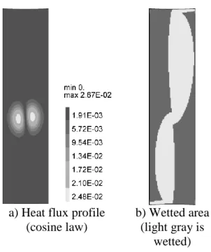
using the cosine law [9,10], possibly adding a cross field heat flux fraction [11]. As a result,
the heat flux profile on the component is known, although in arbitrary units (fig. 2.a). The
actual heat flux entering the component on each node n is q//sepj(n), where q//sep is the parallel heat flux density on the last closed surface. This picture is rendered more complex by
the possible shadowing between components, caused by SOL connections. They are evaluated
for each node n for C by field line tracing (fig. 1) to another component (or more) representing
the rest of the wall (the shadowing component S ), represented by a mesh ({E}S, {N}S), fig. 1.
In the simplified scheme used here, the heat flux is set to zero if a connection is found (full shadowing, c(n) = 0) and c(n) is set to 1 if the field line escapes S (fig. 2.b). The integral of
c(n) over the component gives the wetted area.
The numerical projection of j(n) onto the elements e of {E}C allows calculation of a surface
integral, giving a relation between Ptotal and qsep// :
C // ds p c p j q Ptotal sep . // sep
q is assumed constant for each node n of the component surface and can be factorised.
With discrete formulation, the integral is expressed as a sum and q//sepcan then be obtained
from :
C E e total // sep ) e ( ds ) e ( c ) e ( j P qThe denominator is obtained using a standard software operator. It has the dimension of a
be referred as "parallel heat flux density effective area" (Aef fsep). Having quantified qsep// gives
access to the absolute value of the heat flux everywhere at the surface of the component. The
peak heat flux on the component qmax is the maximum value of the product q//sepj(n)c(n)
over all nodes n {N}C. The peaking factor Pf is then obtained through Pf = qmax A / Ptotal.
This technique is applicable to a set of limiters which are perfectly aligned. In this case, the
calculation is simplified to a single element of the component, assuming toroidal symmetry. If
N is the limiter number, the method is applied to a single limiter element using a power of
Ptotal/N. The method is also applicable to misaligned limiters, the only price to pay being the
loss of toroidal symmetry, with the consequence of much larger meshes and longer run times.
3.
Results for various limiter situations
The model is applied to representative wall situations in an Iter size experiment. A 6.5 MA
limiter plasma is used, the one at the end of the limiter phase in Iter (scenario 2 at 24.17s). For
the modelling presented, the plasma continuously looses Ptotal = 15 MW to the wall. The outer
poloidal curvature radius of this plasma is a = 3 m and the magnetic pitch 7.9°.
The first results are for a series of sets of N outboard poloidal limiters, with N=9, 18 and 36 (a
limiter is represented in fig. 1 with two neighbours at +/- 20°. The neighbours are reduced to
their most forward ridge for simplification, an operation that has no influence of the shadow
frontiers. The geometry of an individual PL is as follows : the intersection of one limiter with
the equatorial plane is an arc, making a 2 centimetre bulge over a toroidal span of 1.5 m. This
corresponds to a radius of 14 m in a horizontal plane. The profile is rotated along a horizontal
axis in the poloidal direction, with a radius of 4.5 m matching approximately the outer
poloidal curvature of the Iter wall. This results in a surface with a double curvature. The area
is A = 10.6 m². The heat flux decay length is prescribed to be 10 mm, an average value
representative of limiter phases in Iter. The number of poloidal limiters (PL) being high, the
pattern and the wetted area are calculated and the results given in table 1. The peaking factor
ranges from 23 to 72, indicating that the peak heat flux is an order of magnitude above the
mean heat flux. The high peaking factor is caused by a combination of factors : the poloidal
curvature mismatch between limiter and plasma, small heat flux decay length and cross
limiter shadowing. The wetted area is a significant fraction of the total limiter area (24% to
53%) : the highest set of limiters (36) has also the smallest wetted (i.e. unshadowed) area
fraction (24%) because of the cross connections between individual limiter segments.
Interestingly, the heat flux on the last closed flux surface is almost constant with the number
of limiters N. Finally, the peak heat load has only as small dependence on the number of
limiters. It can also be noticed that the change of q//sep is only of 17% while the area changes
of 400%. This is a confirmation that the sink action of the limiter set toward the plasma is
well approximated by the one of a toroidal limiter. Should this not be the case, qsep// would
have a much bigger correlation to the limiter number.
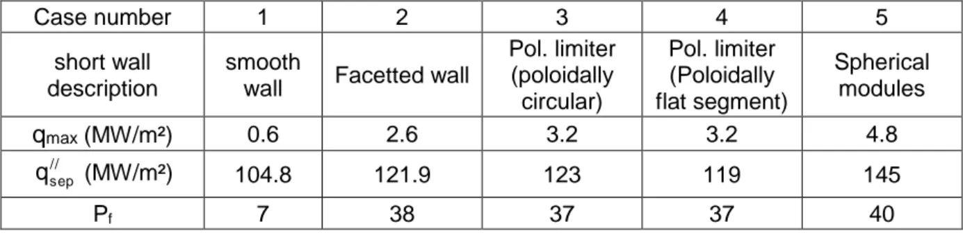
In order to investigate the effect of the local geometry, a series is computed for five wall
surfaces labelled 1 to 5 on the outside, whose results are given in table 2. These wall surfaces
are made to occupy half of the outboard wall to account for 18 equatorial ports (one 10°
sector is occupied every 20°). Case (1) is for a smooth wall made of an outboard toroidal
surface. This case generates no shadow, and the heat pattern is formed of two toroidal bands.
The peak heat flux is multiplied by a factor of 2 to account for the fact that only half of the
wall is used. This is a limiting case, not possible technically, as shaping is required to care for
the leading edges. It is however an lower ideal limit, toward which shape optimisation should
tend. The heat flux is low (0.6 MW/m²) with a Pf of 7, the lowest of all case. Case (2) is a
facetted wall : this wall consists of flat panels in front of each blanket module. The peaking
factor jumps to 38 as the wetted area is reduced by shadowing. It is a significant difference to
(3) is circular in the poloidal direction, as in the previous section. The limiter labelled (4) is
very close to (3) , but is constituted of 1 m flat segments in the poloidal direction to match the
shaping of the first wall modules. This is a shape that matches the current Iter shield modules,
and is a significant design simplification compared to design (3). These two shapes give very
similar results, with Pf ~ 37. This indicates that the price to pay for having straight panels in
the poloidal direction is very small. Case (5) uses a spherical meniscus with a uniform
curvature radius of 14 m, in both poloidal and toroidal directions. This case corresponds to
first wall panel that are shaped in both toroidal and poloidal directions. These produce the
highest peaking factor of 40. As in the previous section, the heat flux on the last closed flux
surface is almost constant (+/- 20%) with the detailed surface shape. This is a remarkable
result, considering the fact that the local geometry is changed of 5 cm, five time p : here also,
this is a confirmation that the toroidal limiter approximation holds for such geometries.
The same technique can be used to investigate the effect of a misaligned component. This is
tested on a inner cylindrical wall of radius R = 5m, of which a sector of 20° is supposed
misaligned by a radial displacement of (Fig. 3). The curvature radius of the bulging module
is adapted so that there is no leading edge. For the case without misalignment ( = 0), the wall
is actually a cylinder, and in that case, the peak heat load can be calculated analytically :
R a e P q p / total max 2 2 2 1
For a = 2.5 m,p = 17 mm this peak heat load is 0.7 MW/m². The peaking factor is calculated
to 3 by assuming a 2 m high wall, making a total surface of 63 m² (the mean heat flux is
15 MW / 63 m² = 0.24 MW/m²) . With increasing , the peak heat flux and the peaking factor
are evaluated using the numerical tool described in section 2. Both peak heat flux and peaking
factor increase with , an intuitive result (table 3). On the regular surface, the peak heat flux
(12% of p) causes a two-fold increase of Pf, while a 20 mm misalignment (slightly above p) creates a peaking factor increase of an order of magnitude. These results are influenced by the shape change with increasing misalignment (the incidence angle on the bulging module is
variable), nevertheless they illustrate the effect of a misaligned element on the power
distribution. This simple case can be used as a benchmark for the various modelling methods.
4.
Conclusion
Given the component geometry and the magnetic field configuration, the exact value of the
peaking factor can be calculated numerically rather than being estimated or guessed. High
values are found for poloidal limiters in Iter sized experiments (usually greater than 10).
These values are caused by the mismatch of curvature radius, as well, of course, the peaking
effect caused by short q. q//sepdoes not vary with the geometrical details of the wall, but
rather with the large scale arrangement. This is a confirmation that for a sufficiently large
number of discrete limiter-objects the plasma-wall contact is well approximated by a toroidal
limiter type geometry, which simplifies the analysis of the wall. Local shaping will be
required to take care of gaps, misalignments (as for the JET Iter-like wall [12]), and of the
long toroidal span caused by the NBI ports in Iter [13]. Nevertheless, such an analyse show
that input power, heat flux decay length and plasma scenario is a sufficient set of data to
References
[1] G. Janeschitz, K. Borrass, G. Federici et al., J. Nucl. Mater., 220-222 (1995) 73-88 [2] A. Kukushkin, H. D. Pacher, M. Baelmans et al., J. Nucl. Mater., 241-243 (1997)
268-272
[3] H. D. Pacher, A. S. Kukushkin, D. P. Coster, J. Nucl. Mater., 266-269 (1999) 1172-1179
[4] M. Kobayashi et Al. Nucl. Fusion 47 (2007) 61-73
[5] X. Bonnin, Ph. Ghendrih, E. Tsitrone et al., J. Nucl. Mater. 337-339 (2005) 395-399 [6] R.A. Pitts, R. Chavan and J.-M. Moret, Nucl. Fus. 39, N°10, (1999) 1433-1449 [7] I. Nunes, P. de Vries and P.J. Lomas, Fus. Eng. Des., 82 (2007) 1846-1853 [8] A. Loarte, S. Bosch, A. Chankin, et al., J. Nucl. Mater. 266-269 (1999) 587-592 [9] R. T. McGrath, Fus. Eng. Des. 13 (1990) 267-282
[10] R. Mitteau, A. Moal, J. Schlosser, et al. J. Nucl. Mater. 266-269 (1999) 798-803 [11] R. Mitteau and Tore Supra team, J. Nucl. Mater. 337-339 (2005) 795-801
[12] M. Firdaouss, R. Mitteau, E. Villedieu et Al., Power deposition on the Iter like wall beryllium tiles at JET., J. Nucl. Mater., 390–391(2009) 947-950
(https://doi.org/10.1016/j.jnucmat.2009.01.243)
[13] P. Stangeby, R. Mitteau, Analysis for shaping the ITER First Wall, J. Nucl. Mater., 390–391(2009) 963-966 (https://doi.org/10.1016/j.jnucmat.2009.01.249)
Fig. 1 : Component mesh Ecomp (1, in black) and shadowing mesh Eshad (2, in gray). Eshad
is the central ridge of Ecomp, rotated from +/- 20° degrees. Two field lines are represented, (i)
escapes the shadowing mesh, and the node of Ecomp from which it originates is designed as
wetted, whereas (ii) connects to neighbour limiter, so that the the node of Ecomp from which
a) Heat flux profile (cosine law)
b) Wetted area (light gray is
wetted)
Fig. 3 : Wall and plasma cross sections in the equatorial plane with a misaligned module. For = 0, the wall is a pure cylinder.
Number of limiters 9 18 36 toroidal span between limiters (°) 40 20 10 Total area (m²) 96 191 382 Wetted area (m²) 51 (9 x 5.66) 74 (18 x 4.12) 100 (36 x 2.78) // sep q (MW/m²) 133 116 113 qmax (MW/m²) 3.6 3.1 2.8* Peaking factor 23 37 72
Table 1 : Results for 9, 18 and 36 outboard poloidal limiters for Ptotal = 15 MW. In the last
Case number 1 2 3 4 5 short wall
description
smooth
wall Facetted wall
Pol. limiter (poloidally circular) Pol. limiter (Poloidally flat segment) Spherical modules qmax(MW/m²) 0.6 2.6 3.2 3.2 4.8 // sep q (MW/m²) 104.8 121.9 123 119 145 Pf 7 38 37 37 40
Mis-alignment (mm) Power on bulging module (MW) Peak heat flux (MW/m²) Reg. heat flux (MW/m²) Pf 0 0.8 (15/18) 0.71 0.71 3 2 1.0 1.5 0.71 6.3 5 1.6 2.8 0.68 11 10 3.0 5.0 0.61 20 20 6.0 9.1 0.45 38
Table 3 : Peak heat fluxes and peaking factors for increasingly bulging modules for