HAL Id: tel-01206478
https://tel.archives-ouvertes.fr/tel-01206478v2
Submitted on 15 Dec 2015HAL is a multi-disciplinary open access archive for the deposit and dissemination of sci-entific research documents, whether they are pub-lished or not. The documents may come from teaching and research institutions in France or abroad, or from public or private research centers.
L’archive ouverte pluridisciplinaire HAL, est destinée au dépôt et à la diffusion de documents scientifiques de niveau recherche, publiés ou non, émanant des établissements d’enseignement et de recherche français ou étrangers, des laboratoires publics ou privés.
arrhythmia treatment using modeling and machine
learning approaches
Rocio Cabrera Lozoya
To cite this version:
Rocio Cabrera Lozoya. Radiofrequency ablation planning for cardiac arrhythmia treatment using modeling and machine learning approaches. Other. Université Nice Sophia Antipolis, 2015. English. �NNT : 2015NICE4059�. �tel-01206478v2�
ÉCOLE DOCTORALE STIC
SCIENCES ET TECHNOLOGIES DE L’INFORMATION ET DE LA COMMUNICATION
T H È S E D O C T O R A L E
pour obtenir le titre de
Docteur en Sciences
de l’Université Nice Sophia Antipolis
Discipline : Automatique, Traitement du Signal et
des Images
Soutenue par
Rocío
Cabrera Lozoya
Planification de l’ablation par radiofréquence des
arythmies cardiaques en combinant modélisation et
apprentissage automatique
Superviseur de thèse: Nicholas AyacheCo-superviseur: Maxime Sermesant
preparé à l’INRIA Sophia Antipolis, Équipe Asclepios soutenue le 10 septembre 2015
Jury :
Président : Pierre Jaïs - Hôpital Haut-Lévêque
et Université de Bordeaux
Rapporteurs : Oscar Cámara Rey - PhySense, Universitat Pompeu Fabra Yves Coudière - Inria (Équipe Carmen)
Examinateur : Jatin Relan - St. Jude Medical, Inc. Superviseur : Nicholas Ayache - Inria (Équipe Asclepios) Co-superviseur : Maxime Sermesant - Inria (Équipe Asclepios)
DOCTORAL SCHOOL STIC
SCIENCES ET TECHNOLOGIES DE L’INFORMATION ET DE LA COMMUNICATION
P H D T H E S I S
to obtain the title of
PhD of Science
of the University of Nice - Sophia Antipolis
Specialty : Automation, Signal and Image
Processing
Defended byRocío
Cabrera Lozoya
Radiofrequency Ablation Planning for Cardiac
Arrhythmia Treatment using Biophysical Modeling and
Machine Learning Approaches
Thesis Advisor: Nicholas Ayache Thesis Co-Advisor: Maxime Sermesantprepared at INRIA Sophia Antipolis, Asclepios Team defended on September 10th, 2015
Jury :
President : Pierre Jaïs - Haut-Lévêque Hospital and University of Bordeaux
Reviewers : Oscar Cámara Rey - PhySense, Universitat Pompeu Fabra Yves Coudière - Inria (Carmen Research Team) Examinator : Jatin Relan - St. Jude Medical, Inc.
Advisor : Nicholas Ayache - Inria (Asclepios Research Team) Co-Advisor : Maxime Sermesant - Inria (Asclepios Research Team)
Abstract:
Cardiac arrhythmias are heart rhythm disruptions which can lead to sudden car-diac death. They require a deeper understanding for appropriate treatment plan-ning.
In this thesis, we integrate personalized structural and functional data into a 3D tetrahedral mesh of the biventricular myocardium. Next, the Mitchell-Schaeffer (MS) simplified biophysical model is used to study the spatial heterogeneity of elec-trophysiological (EP) tissue properties and their role in arrhythmogenesis.
Radiofrequency ablation (RFA) with the elimination of local abnormal ventric-ular activities (LAVA) has recently arisen as a potentially curative treatment for ventricular tachycardia but the EP studies required to locate LAVA are lengthy and invasive.
LAVA are commonly found within the heterogeneous scar, which can be imaged non-invasively with 3D delayed enhanced magnetic resonance imaging (DE-MRI). We evaluate the use of advanced image features in a random forest machine learning framework to identify areas of LAVA-inducing tissue. Furthermore, we detail the dataset’s inherent error sources and their formal integration in the training process. Finally, we construct MRI-based structural patient-specific heart models and couple them with the MS model. We model a recording catheter using a dipole approach and generate distinct normal and LAVA-like electrograms at locations where they have been found in clinics. This enriches our predictions of the locations of LAVA-inducing tissue obtained through image-based learning. Confidence maps can be generated and analyzed prior to RFA to guide the in-tervention. These contributions have led to promising results and proofs of concepts. Keywords: Cardiac electrophysiology modeling, intracardiac electrogram modeling, machine learning, radiofrequency ablation planning, electroanatomical mapping, local abnormal ventricular activities (LAVA)
Résumé:
Les arythmies sont des perturbations du rythme cardiaque qui peuvent entrainer la mort subite et requièrent une meilleure compréhension pour planifier leur traite-ment.
Dans cette thèse, nous intégrons des données structurelles et fonctionnelles à un maillage 3D tétraédrique biventriculaire. Le modèle biophysique simplifié de Mitchell-Schaeffer (MS) est utilisé pour étudier l’hétérogénéité des propriétés élec-trophysiologiques (EP) du tissu et leur rôle sur l’arythmogénèse.
L’ablation par radiofréquence (ARF) en éliminant les activités ventriculaires anormales locales (LAVA) est un traitement potentiellement curatif pour la tachy-cardie ventriculaire, mais les études EP requises pour localiser les LAVA sont longues et invasives.
Les LAVA se trouvent autour de cicatrices hétérogènes qui peuvent être imagées de façon non-invasive par IRM à rehaussement tardif. Nous utilisons des carac-téristiques d’image dans un contexte d’apprentissage automatique avec des forêts aléatoires pour identifier des aires de tissu qui induisent des LAVA. Nous détaillons les sources d’erreur inhérentes aux données et leur intégration dans le processus d’apprentissage.
Finalement, nous couplons le modèle MS avec des géométries du cœur spéci-fiques aux patients et nous modélisons le cathéter avec une approche par un dipôle pour générer des électrogrammes normaux et des LAVA aux endroits où ils ont été localisés en clinique. Cela améliore la prédiction de localisation du tissu induisant des LAVA obtenue par apprentissage sur l’image. Des cartes de confiance sont générées et peuvent êtres utilisées avant une ARF pour guider l’intervention. Les contributions de cette thèse ont conduit à des résultats et des preuves de concepts prometteurs.
Mots clés: modélisation de l’électrophysiologie cardiaque, modélisa-tion d’électrogrammes intracardiaques, apprentissage automatique, planificamodélisa-tion d’ablation par radiofréquence, activités ventriculaires anormales locales (LAVA)
Radiofrequency Ablation Planning for Cardiac Arrhythmia Treatment using Biophysical Modeling and Machine Learning Approaches
Acknowledgments
I would like to start thanking Maxime Sermesant, my PhD supervisor, for your support and encouragement and for the "more than a few" canelés we had at each of our visits to the Bordeaux airport. To Nicholas Ayache, for your constant guidance and for providing a great environment in ASCLEPIOS. It has been a great honor working with both of you.
Thank you to the reviewers, Óscar Cámara and Yves Coudiére, for taking the time to read my thesis (possibly during your holidays) and for your constructive comments which have made this manuscript more complete and readable.
Thank you also to Hubert Cochet, Michel Haïssaguerre, Pierre Jaïs, Benjamin Berte, Yuki Komatsu, Rémi Dubois and everyone else at the CHU Bordeaux, for your invaluable clinical insight and for providing me with data required for my project.
Big thanks as well to Zhong Chen in King’s College London, for always being available to discuss with me and for all your hard work that resulted in the VT chapter of this thesis.
To Jatin Relan, whose guidance was crucial to the success of this work, particu-larly in the first stages of my thesis. To the engineers in the team, Florian Vichot, Loïc Cadour and Hakim Fadil, without whom I would still be stuck compiling MIPS, SOFA and medInria. To all the people with whom I shared an office at some point during my stay in the lab, particularly to Erin Stretton, Krissy MacLeod, Marine Breuilly and Sophie Giffard-Roisin, for the so-very-needed girly talks, chit-chats and gossip.
To people like Jan Margeta and Loïc Le Folgoc, who were always available and very patient to explain to me the various technical concepts with which I struggled more than once.
Isabelle Strobant, for helping me survive the French bureaucracy, which always seemed never-ending!
To everyone else in the team, thank you for the countless BBQs in the beach, climbing sessions, pool parties and our training sessions for the following sports event, be it a marathon, a triathlon or a MudDay!
A big set of very special thanks goes to Eoin, for always believing in me and for being there when I needed it the most!
Last but not least, a mi familia, mis pilares, quienes no han dejado de apoyarme desde el día cero, aún en la distancia. Nada de esto hubiese sido posible sin ustedes. ¡Este es un logro más de los siete fantásticos! ¡Los quiero!
1 Introduction 1
1.1 Clinical Context . . . 1
1.2 Manuscript Organization. . . 3
1.3 Acknowledgment . . . 4
2 Clinical and Technical Context 5 2.1 The Heart: Generalities . . . 5
2.2 Imaging the Heart . . . 10
2.3 Electro-anatomical mapping . . . 10
2.4 Radiofrequency Catheter Ablation . . . 16
2.5 Cardiac Electrophysiology Simulation. . . 19
2.6 Machine Learning in Medical Imaging . . . 21
2.7 Conclusion. . . 25
3 VT Inducibility Prediction: A combined modeling and clinical ap-proach 27 3.1 Introduction . . . 28 3.2 Methods . . . 29 3.3 Statistical Analysis . . . 36 3.4 Results. . . 36 3.5 Discussion . . . 45
3.6 In silico VT stimulation studies in patients . . . 47
3.7 Clinical application . . . 48
3.8 Study Limitations . . . 48
3.9 Conclusion. . . 49
4 Image-based Prediction of Cardiac Ablation Targets 51 4.1 Introduction . . . 52
4.2 Clinical Data . . . 53
4.3 Sources of Uncertainty . . . 55
4.4 Image Feature Computation . . . 56
4.5 Confidence-based Learning Framework . . . 58
4.6 Results and Discussion . . . 61
4.7 Conclusion. . . 65
4.8 Extension to other pathologies . . . 66
5 Image-based Simulation of LAVA Intracardiac Electrograms 67 5.1 Introduction . . . 68
5.2 Clinical Data . . . 68
5.4 Intracardiac EGM Simulation . . . 72
5.5 Signal Analysis . . . 77
5.6 Results and Discussion . . . 77
5.7 Conclusion. . . 83
6 RFA Target Prediction: Combining Imaging Data and Biophysical Modeling 87 6.1 Introduction . . . 88
6.2 Clinical Data . . . 88
6.3 Methods . . . 89
6.4 Evaluation Metrics . . . 90
6.5 Results and Discussion . . . 91
6.6 Conclusion. . . 97
7 Conclusion and Perspectives 99 7.1 Contributions . . . 99
7.2 Methodological and Clinical Perspectives. . . 101
A Spatial Correlation of APD and Diastolic Dysfunction in Trans-genic and Drug-induced LQT2 Rabbits 105 A.1 Introduction . . . 106
A.2 Methods . . . 106
A.3 Results. . . 108
A.4 Discussion . . . 110
A.5 Conclusions . . . 114
A.6 Supplementary data . . . 114
B Personalization of a Cardiac Electromechanical Model using Re-duced Order UKF from Regional Volumes 119 B.1 Abstract . . . 120
B.2 Introduction . . . 120
B.3 Materials and Methods. . . 122
B.4 Results. . . 131
B.5 Discussion . . . 140
B.6 Conclusion. . . 141
B.7 The Bestel-Clément-Sorine electromechanical model . . . 142
C Finetuned Convolutional Neural Nets for Cardiac MRI Acquisition Plane Recognition 145 C.1 Abstract . . . 146
C.2 Introduction . . . 146
C.3 Methods . . . 149
C.4 Validation . . . 157
C.5 Results and discussion . . . 159
Introduction
Contents 1.1 Clinical Context . . . 1 1.2 Manuscript Organization . . . 3 1.3 Acknowledgment . . . 41.1
Clinical Context
Cardiovascular diseases (CVD) refer to the conditions that affect the heart and the circulatory system. To date, they remain the leading cause of death in the western world. According to the Global Burden of Disease, CVD were responsible for more than 29% of deaths in the world in 2013 (> 15,616 million deaths), twice the amount of deaths caused by cancer in the same year [Nichols 2014]. In the European continent alone, despite the recent decrease in CVD deaths, these diseases claim over 4 million victims per year. Figure1.1shows the proportion of non-accidental deaths in Europe in 2013.
Cardiac arrhythmias are a subset of CVD grouping abnormalities in the heart rhythm. A dangerous consequence of these rhythm perturbations includes a com-promise of the heart’s effectiveness to pump blood. Sudden cardiac death (SCD) occurs if the condition is not treated within a short delay. Early detection and accu-rate prediction of disease progression of CVD remain an important need to reduce their mortality. Furthermore, improvements in therapy planning and guidance are of vital importance to reduce the mortality of these diseases.
Depending on the nature of the arrhythmia, either implantable cardioverter-defibrillator (ICD) or radiofrequency ablation (RFA) treatment can be recom-mended. An ICD is a device that continuously monitors the electrical activity in the heart and delivers electrical shocks to control life-threatening arrhythmias. Nonetheless, their effectiveness in reducing mortality is still unclear [Nattel 2014]. Besides, this therapy is a non-curative option and is commonly paired with phar-maceutical treatment. A potentially curative alternative is RFA treatment, where thermal lesions are generated in the heart to interrupt abnormal re-entry circuits that cause arrhythmias. The greatest challenge in this therapy is ablation target identification. Currently, this can be achieved using electrophysiological (EP) sub-strate mapping. Recently, [Jaïs 2012] showed that the elimination of local abnormal
ventricular activities (LAVA) was an effective endpoint for substrate-based ventric-ular tachycardia.
Figure 1.1: Proportion of all deaths due to major causes in Europe (Top) among men and (Bottom) among women. Courtesy of [Nichols 2014]
The main questions we aim to answer in this thesis are:
- Can personalized structural and functional data help us understand the patient-specific arrhythmogenesis?
- Can appropriate imaging data provide us with information to characterize and identify RFA targets?
- Are we able to use non-invasive image-based models and in silico simulation to generate intracardiac electrograms with LAVA-like patterns at the locations where they have been found in clinics?
- Can these simulated electrograms enrich the predictions of RFA targets ob-tained through image-based learning?
1.2
Manuscript Organization
This thesis is based on our published and submitted work, Figure 1.2 exemplifies the manuscript organization.
Figure 1.2: Manuscript Organization.
In Chapter 2, we introduce the relevant clinical concepts for understanding this work and review the state of the art of electrophysiology modeling and the use of machine learning schemes in the medical domain.
In Chapter 3, based on [Cabrera-Lozoya 2015c], we make use of integrated personalized structural and functional data to study the spatial heterogeneity of electrophysiological tissue properties and their role in arrhythmogenesis.
In Chapter 4, based on [Cabrera-Lozoya 2014] and on [Cabrera-Lozoya 2015d], we evaluate the predictive power of locally computed intensity and texture-based MRI features to identify radiofrequency ablation targets using a machine learning framework, including a detailed analysis of the dataset’s inherent error sources and their integration in the training process.
In Chapter 5, based on [Cabrera-Lozoya 2015a], we test the feasibility of us-ing delayed enhanced MR image-based models to reproduce LAVA-like patterns in simulations of catheter recordings of intracardiac electrograms.
In Chapter 6, based on [Cabrera-Lozoya 2015b], we present a proof of con-cept where in silico simulated electrograms enhance the predictions of RFA targets obtained through MR image-based learning.
Finally, in Chapter 7, we conclude this thesis by describing our main contribu-tions and perspectives.
In the appendices, we present additional fruitful collaborations carried out during the time of the PhD but which go beyond the scope of this thesis.
1.3
Acknowledgment
Part of this work was funded by the European Research Council through the ERC Advanced Grant MedYMA 2011-291080 (on Biophysical Modeling and Analysis of Dynamic Medical Images).
Clinical and Technical Context
Contents
2.1 The Heart: Generalities . . . 5
2.1.1 Cardiac Anatomy. . . 5
2.1.2 Cardiac Electrophysiology in the Healthy Heart . . . 6
2.1.3 The Pathological Heart . . . 8
2.2 Imaging the Heart . . . 10
2.3 Electro-anatomical mapping . . . 10
2.3.1 Mapping Systems. . . 11
2.3.2 Electrogram Interpretation . . . 13
2.3.3 Mapping Approaches. . . 15
2.4 Radiofrequency Catheter Ablation . . . 16
2.4.1 Ablation Target Identification Up Until Now . . . 16
2.4.2 Endpoints for RFA Therapy. . . 17
2.5 Cardiac Electrophysiology Simulation . . . 19
2.5.1 The Mitchell-Schaeffer Model . . . 20
2.6 Machine Learning in Medical Imaging . . . 21
2.6.1 Random Forests for Classification. . . 22
2.7 Conclusion . . . 25
In this thesis, we use mathematical modeling and machine learning techniques alongside with patient-specific clinical data to guide radiofrequency ablation therapy for the treatment of cardiac arrhythmias. In this chapter, we review the essentials and basics of the clinical aspects and mathematical techniques.
2.1
The Heart: Generalities
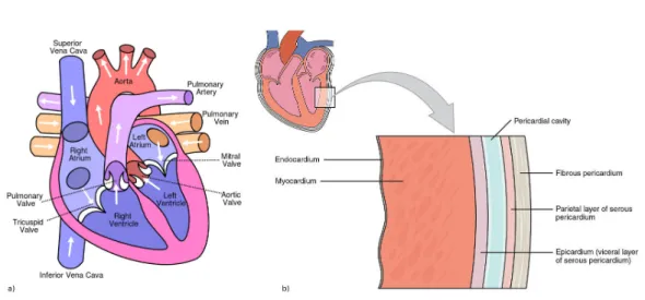
2.1.1 Cardiac AnatomyThe heart is the muscular organ responsible for pumping blood through the car-diovascular system, providing the body with oxygen and nutrients while removing metabolic waste. It is enclosed in a protective sac called the pericardium, which prevents overfilling of the heart and helps it anchor to the surrounding structures in the mediastinum in the chest.
Figure 2.1: a) Heart anatomy and chambers. b) Layers of the heart wall. From
en.wikipedia.org/wiki/Heart.
The heart is composed of four chambers: the left and right atria (upper, blood-receiving chambers) and the left and right ventricles (lower, blood-discharging cham-bers) as shown in Figure 2.1a. Blood from systemic circulation flows through the superior and inferior vena cavae into the right atrium, across the tricuspid valve and into the right ventricle. Then, the blood crosses the pulmonary valve and passes into the pulmonary circulation in direction of the lungs. Once metabolic wastes are removed from the blood and oxygen is added, it will return to the left atrium, through the mitral valve and into the left ventricle before being discharged again to the systemic circulation through the aorta.
The heart wall is divided in three layers shown in Figure 2.1b, the outer-most layer is called the epicardium, the middle one composed mainly of cardiac muscle responsible for heart contraction is referred to as the myocardium and the inner layer, the endocardium, is in direct contact with the blood. Heart muscle cells, myocytes, are arranged in fibers whose direction varies across the myocardium. The fiber orientation can be described by an elevation angle corresponding to its obliquity with respect to the plane of the section. The value of this angle varies from approximately +70◦ on the endocardium, 0◦ in mid-myocardium to −70◦ in the
epicardium (Figure 2.2). This swirled organization optimizes the pumping function of the heart.
2.1.2 Cardiac Electrophysiology in the Healthy Heart
An adult human heart at rest contracts with a stable rhythm of approximately 60-100 beats per minute (bpm). This sinus rhythm is managed by the automaticity of the heart’s natural pacemaker, the sinoatrial (SA) node, which is a group of cells capable of spontaneously generating electrical signals that propagate through the heart muscle. The electrical wave travels first through the atrial fibers (the pathway propagating the electrical impulse to the left atrium is known as the Bachmann’s
Figure 2.2: Human ventricular fibers from in vivo Diffusion Tensor Imaging (DTI). Fibers are color-coded with the local helix angle α. Courtesy of team.inria.fr/ asclepios.
bundle) and to the atrioventricular (AV) node. Here, a delay allowing an appropriate filling of the ventricles during the atrial contraction takes place. Thereafter, the electrical stimulus travels through the His bundle into the left and right bundle branches. Finally, the Purkinje network allows the activation of the cardiac myocytes in the ventricles. A schematic of the heart’s conduction system is found in Figure
2.3.
Figure 2.3: Heart’s conduction system. Fromen.wikipedia.org/wiki/Heart.
In non-pathological conditions, a cardiac cell has a resting polarized state, mean-ing that there exists an electrical potential difference, typically of -90mV, across the cell membrane separating the intracellular and extracelluar mediums. When the cell receives an electrical stimulus (like the wave arising from the SA node), its trans-membrane potential evolves in accordance with the gradient of ionic concentrations inside and outside the cell. The temporal evolution of the transmembrane potential
is known as an action potential and it consists of three main phases (Figure 2.4): 1. Depolarisation: Fast Na+channels open and sodium ions can enter the cell,
rapidly rendering its inside positive with respect to the extracellular medium. 2. Plateau: K+ and Na+ channels are slowly de-activated and Ca2+ ones are
opened, momentarily stabilizing the transmembrane potential.
3. Repolarisation: The K+ channels gradually re-activate and there is a
de-crease in the calcium influx, re-establishing the ionic rest state of the cell.
Figure 2.4: (Left) Simplified schematic of ionic flow through the cell membrane. (Center) Evolution of ionic conductances. (Right) Action potential (mV). Courtesy of [Talbot 2014]
2.1.3 The Pathological Heart Myocardial Infarctions
In pathological cases, an interruption of the blood supply to the cardiac tissue can occur. The main cause of this phenomenon is the occlusion of one of the blood vessels irrigating the heart, known as the coronary arteries. If left untreated, oxygen-deprived cells can suffer from irreversible damage or even death (myocardial infarction, MI). Areas adjacent to the necrotic core are referred to as the border zone, where surviving myocytes are surrounded by dense fibrosis, as seen in Figure
2.5. These areas present decreased lateral connection between the myocardial cells, which undergo changes in the transmembrane ion channel expression leading to differences in their electrophysiological behaviors [Rutherford 2012]. These disrup-tions can potentially cause abnormal heart beating patterns (cardiac arrhythmias) or even a complete stopping of the heartbeat, a condition known as cardiac arrest. Cardiac Arrhythmias
A cardiac arrhythmia is a broad classification of the conditions that perturb the normal cardiac rhythm, rendering it either irregular, too slow or too fast. Of particular interest for this thesis are ventricular tachycardias, which are character-ized by an abnormally fast (from 120 up to 280 bpm) heart rhythm originating
Figure 2.5: Three-dimensional reconstruction of infarct border zone. (Left) Short-axis slice cut 4mm of the left ventricular apex. Collagen is indicated in white/yellow and myocytes by red/brown. (Right) Reconstructed infarct border zone. The dimen-sions of the image volume are 2.99×2.68×0.70mm3. Courtesy of [Rutherford 2012]
in the ventricles. They can degenerate into ventricular fibrillation and cause an uncoordinated contraction of the cardiac muscle, compromising heart function and potentially leading to sudden death.
Scar-related ventricular tachycardia (VT) or arrhythmia
The presence of scar in the myocardial tissue can lead to abnormal electrical cir-cuit generations, often referred to as scar-related reentry [Aliot 2009]. Although the main cause for scar formation reported is myocardial infarction [Stevenson 1993], other conditions can result in damaged myocardial tissue, including arrhythmogenic right ventricular cardiomyopathy (ARVC) [Belhassen 1984], dilated cardiomyopathy
[Hsia 2002] or surgery [Eckart 2007]. Myocardial scar can be identified due to its
electrophysiological characteristics, which include low-voltage regions or fraction-ated electrograms, or through imaging studies. According to [Aliot 2009], substrate promoting scar-related re-entry can have the following characteristics:
- Regions of slow conduction.
- Unidirectional conduction block at some point in the re-entry path that allows initiation of re-entry.
According to animal [El-Sherif 1981] [El-Sherif 1983] and human
[De Bakker 1988] studies, the phenomenon of re-entry is due to the existence
of surviving myocyte bundles and the increased presence of collagen and connective tissue affecting their coupling with the rest of the myocardium. This perturbation of normal myocardial architecture promotes abnormal patterns of activation and conduction velocity [Peters 1998].
2.2
Imaging the Heart
In patients with suspected scar-related VT, imaging studies can be used to assess the viability of the myocardial tissue, as well as to obtain important aspects of tissue heterogeneity, scar extent and location. Delayed-enhanced (DE) magnetic resonance imaging (MRI), which has the advantage of being a non-ionizing imaging technique, is used in conjunction with gadolinium (Gd) as a contrast agent to improve scar vi-sualization. Nonetheless, DE-MRI is often prohibited in VT-prone patients because many of them have implanted pacemakers or ICDs. Also, the presence of these devices can lead to important artifacts and deteriorate image quality. The use of DE multi-detector computed tomography (MDCT) has been investigated in these cases, but its reproducibility is still debated [Aliot 2009].
To date, DE-MRI remains the gold standard for myocardial size and mor-phology evaluation, it is also used to assess the heterogeneity of the border zone
[Schuleri 2009]. Figure 2.6 exemplifies the use of DE-MDCT and DE-MRI in
an-imal subjects for visualizing the scar and border zone (also known as peri-infarct zone) and their correlation with histological cuts.
2.3
Electro-anatomical mapping
Electroanatomical mapping (EAM) is a minimally-invasive technique used to record in-vivo cardiac electrical activity at specific locations inside the heart. The method of entry is chosen according to the cardiac chamber to be studied. When the cavity of study is the right part of the heart, then the mapping catheter is introduced through the femoral vein. Alternatively, when studying the left heart, the femoral artery is chosen. When the catheter either comes in contact with the tissue of interest or is located within its vicinity, both the electrical activity of the tissue and the coordinates of the catheter’s position in space are retrieved. These systems integrate three main functions [Aliot 2009]:
- Non-fluoroscopic localization of the ablation catheter within the heart
- Display of electrogram characteristics (i.e. activation time or voltage) w.r.t. anatomic position
- Integration of electroanatomic information with 3D images of the heart ob-tained from computed tomography (CT), magnetic resonance imaging (MRI) or other imaging technique.
Figure 2.6: Example of matching histological data in chronic infarcts against DE-MDCT (A and B) and DE-MRI (D and E). The peri-infarct zone (PIZ) is visualized between tow black arrows by intermediate signal intensity (white circle) in DE-MDCT images. In D and E, DE infarct scar (white arrows) and the PIZ (white circle) show different signal intensity in DE-MRI. (C and F) Masson trichrome stain depicts viable myocardium in red (∗) from non-viable tissue in blue. At higher magnification (F) the islands of viable myocytes (red) within the scar tissue are visualized, showing the heterogeneity of the PIZ. Image from [Schuleri 2009].
Despite the capability of locating the catheter in 3D space and therefore re-constructing the heart chamber that is being mapped, geometries provided by EAM systems tend to be rough estimates of the actual cardiac anatomy. Catheter position is highly affected by cardiac or respiratory motion, and anatomic reconstruction al-gorithms may vary between systems [Aliot 2009]. These limitations can compromise the integration of EAM information with anatomical information from traditional imaging systems. Often, multiple mapping catheters are used in order to improve spatial sampling.
2.3.1 Mapping Systems
Two main types of mapping systems currently exist in the clinical market: contact mapping and non-contact mapping.
Figure 2.7: CARTO navigation system with (Left) fluoroscopic images, (Center) CARTO contact mapping catheters and (Right) the electroanatomical mapping. (Images from CHU, Bordeaux)
EP Contact Navigation System (Biosense Webster Inc.), shown in Figure 2.7. As the name implies, this mapping technique requires direct contact between the recording catheter and the cardiac tissue. The catheter is moved along the endocardial or epicardial wall to capture electrical signals. It is preferred for the study of local phenomena. The three-dimensional location of the catheter in this particular system is achieved through the placement of three coils beneath the patient producing low-level electromagnetic fields which are measured by a sensor located at the tip of the mapping catheter, which have reported a magnitude of location errors from the catheters of ∼ 1mm [Gepstein 1997]. In some applications throughout this thesis, the contact mappping system was used in conjunction with a multi-spline recording catheter (PentaRay, Biosense Webster) having a five-branched star design which allows for high-density mapping, it is shown in Figure 2.8.
Figure 2.8: PentaRay multi-spline recording catheter. (Image from BioSense Web-ster Inc.)
Non-contact Mapping: The EnSite Velocity System (St. Jude Medical Inc.), shown in Figure2.9, is part of the non-contact mapping systems. In this approach, the recording device consists of a catheter with a multi-electrode array of 64 unipo-lar electrodes over an inflatable balloon, each of which can remotely measure the potential generated by far-field electrograms [Aliot 2009]. Because the electrical ac-tivity does not correspond to the potentials at the endocardial surface but in the blood pool, an inverse problem must be solved. Virtual unipolar electrograms at the endocardium are accurately reconstructed and in agreement with contact mapping recordings if the surface of interest is within 4 cm of the center of the MEA balloon
[Gornick 1999] [Schilling 1998] [Sivagangabalan 2008]. Because of these
character-istics, the system is preferred for activation mapping. It also has the advantage of being applicable in patients who cannot tolerate arrhythmia or when an arrhythmia cannot be reproduced during the EP study.
Figure 2.9: EnSite navigation system with (Left) fluoroscopic images, (Center) the deflated and inflated balloon and (Right) the electroanatomical mapping. (Images from KCL, London)
2.3.2 Electrogram Interpretation
Aside from the mapping system chosen for a given procedure, it is of vital impor-tance for the clinical electrophysiologist to be able to recognize complex patterns in recordings inherent to the nature of the electrograms (EGM), in order to accurately diagnose and locate arrhythmias [Stevenson 2005].
Cardiac electrograms are the voltage differences between two recording elec-trodes (a positive lead, known as the anode, and a negative lead, referred to as the cathode) at a given point in the cardiac cycle [Stevenson 2005]. There exist two main kinds of electrograms recorded during EAM: unipolar and bipolar.
Unipolar electrograms: When recording unipolar electrograms, the anode is in contact with the myocardial tissue of interest and the cathode is placed at a distant point from the heart, such that its influence in the cardiac measurements is negligible. Although theoretically the cathode should be placed at an infinite
distance from the heart to obtain a truly unipolar recording, in practice, it is located in the inferior vena cava [Stevenson 2005]. Following this convention of electrode placements, a depolarization wavefront moving towards the electrode in the cardiac chamber will result in a positive deflection in the EGM, whereas a receding one will yield a steep negative deflection. The point of maximum negative slope (−dV/dt) corresponds to a wavefront directly underneath the recording electrode
[Stevenson 2005]. This characteristic renders unipolar electrograms valuable for
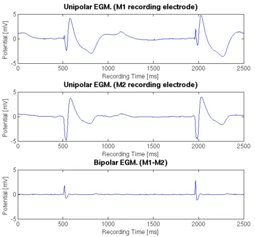
the generation of activation maps and to identify the site of earliest activation in focal tachycardias. One major limitation of unipolar electrograms is the effect of far-field signals from depolarising myocardial tissue at the distance [Aliot 2009], this is particularly hindering in scar regions where the local low-voltage potentials can be overshadowed by far-field effects. Sample unipolar electrograms are shown in the top and middle rows of Figure 2.10.
Figure 2.10: Sample unipolar (top and middle) and bipolar (bottom) intracardiac electrograms obtained from the CARTO navigation system.
are generated by computing the difference in the potential recorded between two closely-spaced electrodes. Local activation is identified by the initial signal peak, but this measure is less reliable than with unipolar electrograms if the signals are fractionated or have multiple components. The far-field signals in the two electrodes is considered equivalent, therefore bipolar EGMs are useful to evaluate local signals
[Stevenson 2005], even those with low-amplitude potentials, making them ideal for
mapping scar-related arrhythmias [Aliot 2009].
Most catheters are equipped with four electrodes numbered from 1 to 4 from the distal-most to the proximal-most. Comparisons between the bipolar signals generated by neighboring electrodes indicate wavefront direction, but the amplitude of the signals can be severely compromised if the wavefront is moving perpendicular to the axis of the recording dipole.
In order to better exploit the strengths of both types of electrograms, EP studies usually obtain both unipolar and bipolar recordings simultaneously.
2.3.3 Mapping Approaches
Different mapping approaches can be used to study a particular type of arrhythmia in a given patient, though they are often complementary. This section describes the most commonly used ones:
Activation Mapping: Consists in the recording of the electrical activation sequence of the chamber of interest. It is necessary to establish both a location and timing reference, as well as a timing window. Although in theory either intracardiac EGMs or surface ECG leads can be used to chose a timing reference, intracardiac EGMs are preferred [Bhakta 2008].
Pace Mapping: During this approach, a site of interest is paced during the absence of VT and the resulting activation sequence and surface ECG morphology are assessed. If the pacing of a particular site reproduces the same ECG morphology as the one seen during clinical VT, then the location is suspected to be either the origin of a focal VT or the exit of a scar-related re-entry [Brunckhorst 2004]. Entrainment Mapping: Is performed by delivering a train of stimuli at a rate just higher than the one present during VT [Stevenson 1993]. It serves to identify re-entry circuits sites, e.g. surface ECG morphology during entrainment will determine if the pacing site is within an isthmus or not [Aliot 2009].
Substrate Mapping: Refers to the characterization of a region of interest, particularly those suspected to promote re-entry due to their anatomical or elec-trophysiological characteristics. Scarred tissue is frequently the target of substrate mapping and its correlation with low-voltage areas has been found in animal models [Callans 1999]. Regions with particularly low-voltage (<0.5mV) have been referred to as dense scar but can still participate in re-entry circuits as they can
contain varying amounts of viable myocytes [Soejima 2002]. Furthermore, targeting the border zone for ablation, which consists of regions with voltage ranging from 0.5 to 1.5 mV, has gained interest in the recent years [Marchlinski 2000] [Aliot 2009].
2.4
Radiofrequency Catheter Ablation
Radiofrequency ablation (RFA) is a technique in which a tissue region is subjected to extreme heat resulting from a high-frequency alternating current
[Townsend Jr 2012]. In cardiology, it is used to destroy electrical pathways
respon-sible for cardiac arrhythmias. The extent of the RFA lesion created is dependent of operator-controlled characteristics, such as RF power and duration (which should be at least 35 to 45 seconds to approach steady state [Haines 1993]), but also on operator-independent phenomena, including electrode-tissue contact and the cool-ing effect by the circulatcool-ing blood [Haines 1993]. Temperature monitoring is very important in order to ensure a proper ablation of the target site while minimizing the risk of serious complications such as of thromboembolism, although these are infrequent [Matsudaira 2003].
RFA is considered the sole treatment option for patients suffering from recurrent ventricular tachycardias (VT) without structural heart disease [Aliot 2009]. Pa-tients with scar-related VTs are also referred for RFA therapy in conjunction with implantable-cardioverter defibrillators (ICDs) and/or anti-arrhythmic drug therapy
[Aliot 2009]. RFA ablation is a complex intervention reserved to patients with
ad-vanced heart disease [Aliot 2009]. The percentage of significant complications (re-quiring prolonged hospitalization, additional interventions or death) reported in
[Reddy 2007] was of < 5% on patients undergoing prophylactic catheter ablation of
post-infarction VT in a randomized, multi-center study.
2.4.1 Ablation Target Identification Up Until Now
Though RFA has proven to be an effective therapy in patients suffering from ventric-ular tachycardia (VT) whose ICD triggers frequent defibrillation shocks [Aliot 2009], to date, there exists no universal consensus on the optimal ablation strategy.
A number of techniques are found in the literature to treat either unmappable or hemodynamically intolerable VT. Studies such as [Marchlinski 2000] reported the use of linear endocardial RFA lesions going from the regions of dense scar to those of normal myocardium to control unmappable VT. [Kottkamp 2003] described how 80% of the 28 patients in their study were rendered non-inducible after the placement of line lesions that transected all potential isthmuses. The study in [Soejima 2001] also used lines of RF lesions to treat unstable VT and suggested that less ablation is needed when a reentry circuit isthmus is identified.
Furthermore, reentry isthmuses can be identified in a number of ways. In
[Soejima 2002], these were located by identifying electrically unexcitable scar within
where an abrupt change in paced QRS morphology is hypothesized to be an index of a successful ablation target in patients with well-tolerated post-infarct endocardial re-entrant VT [De Chillou 2014] or through pace-mapping within the scar tissue with the aim of identifying electrogram characteristics that are helpful for isthmus identification during sinus rhythm, as done in [Bogun 2006]. The authors explained how good pace maps at the sites of isolated potentials within the scar identify parts of the critical isthmuses in post-infarction VT patients.
Voltage maps and local electrogram voltage characteristics have also been stud-ied in the identification of slow conduction channels responsible for re-entrant cir-cuits. The study in [Hsia 2006] defined a conducting channel as a path of multiple activated sites within the VT circuit that demonstrated an electrogram amplitude higher than that of surrounding areas and concluded that most entrance and isth-mus sites of hemodynamically stable VT are located in dense scar, whereas exits are located in the border zone. Nonetheless, these approaches require a careful voltage threshold adjustment. In [Arenal 2004], the effect of different levels of voltage scar definition in the identification of conducting channels inside the scar was studied in a patient cohort with chronic myocardial infarction referred for VT ablation. Although most of the conducting channels were identified by defining the voltage scar with a threshold of ≤ 0.2mV and RFA supressed the inducibility in 88% of the tachycardias, they concluded that a tiered decreasing-voltage definition of the scar is critical for channel identification. [Di Biase 2012] suggested an aggressive scar homogenization technique in which all abnormal electrograms were targeted, with successful results in endo-epicardial applications. Others, like [Tilz 2014] described how the use of linear ablations encircling the scar would yield its electrical isolation and had promising results in VT treatment.
2.4.2 Endpoints for RFA Therapy
Traditionally, VT non-inducibility is still considered the endpoint in RFA treatment. According to [Aliot 2009], three general endpoints to catheter ablation have been evaluated:
1. Non-inducibility of clinical VT
2. Modification of induced VT cycle length (elimination of all VTs with cycle lengths ≥ spontaneously documented or targeted VT)
3. Non-inducibility of any VT (excluding ventricular flutter and fibrillation) Nonetheless, these are not guaranteed to be the optimal RF ablation endpoints and debate still exists in their use for assessing ablation lesion creation [Aliot 2009]. Alternative Endpoints to RFA Therapy: In recent years, new endpoint strate-gies have been proposed. For the treatment of VT in 18 patients with arrhythmo-genic right ventricular cardiomyopathy (ARVC), [Nogami 2008] evaluated the mod-ification of RFA therapy endpoint to the change in isolated delayed components
T able 2. 1: Strategies fo r substrate-guid ed VT ablation. Ablation Design Mano euv ers for Substrate Pro cedure Extension Isthm us Iden tification Ablation T arget Endp oing of RF Ablation Lines Linear ablation from P acemapping Scar b order zone Non-inducib ilit y + + + + [ Marc hlinski 20 00 ] dense sca r to normal m yo cardium Electrically unexcitable Short lines P acem apping Channels b et w een Non-inducibilit y + + scar mapping unexcitable scars [ So ejima 2001 ] V oltage defined Sh ort lines P acemapping Chann els b et w een Non-ind ucibilit y or + + conducting ch annel conducting cha nnels disapp earance or [ Arenal 2004 ] isolated Scar homogeneization Clouds of RF applicatio ns Not required All abnormal Non-inducibilit y + + + + [ Di Bi ase 2012 ] electrograms LA V A ablation P oin t by p oin t ablati on Not required LA V A LA V A Elimination + + + [ Jaïs 2012 ] Circumf eren tial Circumf eren tial abl ation Not required Scar b ound aries Scar isolati on + + + scar isolation [ Tilz 2014 ] Non-exhaustiv e review of prop osed strategies for substrate-guided VT ablation. Mo dified from [ Berruezo 2014 ]
(IDC). They concluded both that IDCs that appear in sinus rhythm are related to clinical VT and can therefore be used as ablation targets and that a change in IDC was a possible endpoint to the therapy due to the siginficantly lower VT recurrence in patients who presented it with respect to those with no IDC or unchanged IDC. A recent study with a larger cohort of 70 patients suffering from VT and struc-turally abnormal ventricles proposes the elimination of local abnormal ventricular activities (LAVA) as an endpoint for RFA therapy [Jaïs 2012]. The clinicians ablated LAVA found through the use of a high-density mapping catheter during both sinus rhythm or ventricular pacing and concluded that their elimination was associated with a reduction in recurrent VT or death during long-term follow-up [Jaïs 2012]. Table 2.1 presents a non-exhaustive review of proposed strategies for substrate-guided VT ablation.
2.5
Cardiac Electrophysiology Simulation
There exist several models for computing cardiac electrophysiology ranging from highly complex to fairly simple. They can be broadly classified into three groups: biophysical models, phenomenological models and Eikonal models.
- Biophysical models deal with a highly complex modelling of the differ-ent ionic concdiffer-entrations and channel dynamics at a cellular level and can include over 50 variables; an example of them is the ten Tusscher model [K. ten Tusscher 2004].
- Phenomenological models often appear as simplifications of the biophysi-cal models, with a consequent reduction in the number of involved variables. Nonetheless, they are still able to capture the shape of the action poten-tial and are useful to model the propagation at the organ scale. The Aliev-Panfilov [Aliev 1996], Fenton-Karma [Fenton 1998], FitzHugh [FitzHugh 1961] and Mitchell-Schaeffer [Mitchell 2003] models belong to this group. These models can be further classified into bi-domain or mono-domain. Bi-domain models consider an intracellular and an extracellular domain separated by the cell membrane but which remain overlapping and continuous. It models the evolution of the potentials in both domains separately. Mono-domain models, on the contrary, assume the extracellular potential is grounded. Therefore, the intracellular potential is equal to that of the membrane.
- Eikonal models [Keener 1991] correspond to static non-linear partial differ-ential equations of the depolarisation time derived from the previously men-tioned models. They are not able to account for complex physiological states. These models have been used for numerous applications [Trayanova 2011] varying from the study of the normal wave propagation in the ventricles
[Simelius 2001] and the effect of repolarization parameter heterogeneity across the
heart [Franzone 2008] to the understanding of the organization of human ventricular fibrillation to identify potential therapeutic targets [Ten Tusscher 2009].
2.5.1 The Mitchell-Schaeffer Model
Throughout this thesis, the Mitchell-Schaeffer (MS) model was used to model car-diac electrophysiology. It is a simplified biophysical model derived from the Fenton-Karma ionic model [Mitchell 2003] [Fenton 1998]. It has found applications in patient-specific personalisation for VT simulation [Relan 2011a] and interactive sim-ulator generation of patient-specific electrophysiology [Talbot 2014].
It models the transmembrane potential as the sum of a passive diffusive cur-rent and several active reactive curcur-rents including a combination of all inward and outward phenomenological ionic currents. This is described in the MS model by a system of partial differential equations:
∂tu = div(D∇u) +zu 2(1−u) τin − u τout + Jstim(t) ∂tz = ( (1−z) τopen if u < ugate −z τclose if u > ugate (2.1) Where:
u is a normalized transmembrane potential variable
z is a gating variable which depicts the depolarization and repolarization phases by opening and closing the currents gate
zu2(1−u)
τin represents the inward currents, Jin, which raise the action potential
voltage (primarily Na+ and Ca2+) u
τout represents the outward currents, Jout, that decrease the action potential
voltage (mainly K+), describing repolarization
Jstim is the stimulation current at the pacing location
τin, τout, τopen, τclose have units of seconds
D is a diffusion tensor that controls the diffusion term in the model
This model incorporates both action potential duration (APD) and conduction velocity (CV) restitution effects, and the restitution curves can be written in an analytical formulation.
APD restitution. It is an electrophysiological property of the cardiac tissue and defines the adaptation of APD as a function of the heart rate. Its slope has a heterogeneous spatial distribution. The APD restitution curve (APD-RC) defines the relationship between the diastolic interval (DI) of one cardiac cycle and the APD of the subsequent cardiac cycle. The slope of these RCs is controlled by a model parameter τopenof the MS model and depicts the APD heterogeneity present
AP Dn+1 = f (DIn) = τcloseln( 1 − (1 − hmin)e −DIn τopen hmin ) (2.2)
where hmin = 4(τin/τout) and n is the cycle number. The maximum value of
APD is also explicitly derived as:
AP Dmax= τcloseln(
1 hmin
) (2.3)
CV restitution. This formulation is also present in the MS model. Its mathe-matical formulation is described in the following equation, with g(DI) = CV as the next cycle CV: g(DI) = (1 4(1 + s 1 − hmin h(DI)) − 1 2(1 − s 1 − hmin h(DI)) s 2dh(DI) τin ) (2.4)
2.6
Machine Learning in Medical Imaging
Deriving realistic mathematical models to explain complex physiological phenomena can sometimes prove to be a difficult task. Machine learning is a branch of artificial intelligence whose aim is the generation of algorithms capable of learning from ob-servations in order to make predictions about future ones. It has found applications in fields as varied as language processing [Collobert 2008] [Daelemans 2003], com-puter vision [Taigman 2014] [Huang 2008] or stock market analysis [Huang 2005]
[Schumaker 2009]. Its increased use by the medical imaging community is due to
the processing of high volumes of multi-dimensional data, including uncertainty and noise, coming from multi-modal sources that exist in this domain. Nonetheless, one of the main challenges is the generation of ground truth, as it requires the annota-tion of large volumes of data by a set of medical experts. Therefore, large efforts are continuously being made to provide clinicians with user-friendly and efficient annotation tools.
Among the various applications of machine learning techniques in the medi-cal field are detection or segmentation of anatomimedi-cal structures [Criminisi 2011a]
[Geremia 2013], registration [Muenzing 2012] [Aljabar 2012] and image recognition
[Margeta 2015].
Classification tasks are among the functions that machine learning techniques are used for and many of such algorithms exist in the literature. One of the most widely used is the support vector machines (SVM) classifier because it guaran-tees maximum-margin separation in binary classification tasks. Boosting also ranks among the most popular techniques and works by building a strong classifier as a linear combination of many weak ones. Random forests have emerged as a machine learning technique that can simply and effectively combine randomly trained classi-fication trees and has been shown to be easily extendable to multiple class problems [Criminisi 2011a].
Figure 2.11: Classification: Training data and tree training. a) Input data points. The ground truth label of training points is denoted with different colors. Grey circles indicate unlabeled, previously unseen test data. b) A binary classifica-tion tree. During training a set of labeled training points {v} is used to optimize the parameters of the tree. In a classification tree the entropy of the class distributions associated with different nodes decreases (the confidence increases) when going from the root towards the leaves. Courtesy of [Criminisi 2011a]
2.6.1 Random Forests for Classification
Random forests are discriminative classifiers that generate a hierarchical represen-tation of the training data which is optimized for testing. They have been chosen as the machine algorithm framework of this thesis because, unlike state-of-the-art classifiers such as SVMs, they are created in an intuitive and easily understandable structure. Moreover, they also provide informative uncertainty measures on the clas-sification results [Criminisi 2011a], which would only be possible with probabilistic SVM implementations such as the relevance vector machine at the expense of com-putational efficiency. They also possess maximum-margin properties, the hallmark of SVMs, implicitly incorporate the notion of bagging into their framework and compare to boosting techniques by building strong classifiers from a large number of weaker ones. This framework has already successfully found multiple applica-tions in the medical image processing community, such as brain lesion segmentation
[Geremia 2013], myocardium delineation in 3D echocardiography [Lempitsky 2009],
segmentation of the left atrium in 3D MRI [Margeta 2014b] and organ localization in CT volumes [Criminisi 2011a].
The goal in classification is to automatically associate an input data point v with a discrete class c ∈ {ck}. Machine learning algorithms have proven to
be powerful tools to discover the relevant correlations within a dataset and to design a classification method based on the most discriminant features. The training data consists of a set of labeled observations T = vk, Y (vk) where the
domain. When asked to classify a new input observation, the classifier aims to assign it a label y(v). The process of classification can be divided into an of-fline training phase and an online testing phase, both of which will be described next. Training phase
During training, exemplified in Figure2.11, the algorithm optimizes the param-eters of the weak learner at each split node (j):
θ∗j = argmax Ij θj∈τj
(2.5) where the objective function Ij is the information gain for discrete distributions:
Ij = H(Sj) − Σ i∈L,R | Si j | | Sj | H(Sji) (2.6)
with i ∈ L, R representing the left and right child nodes. The term H(S) corre-sponds to the Shannon entropy:
H(S) = − Σ
c∈Cp(c) log p(c) (2.7)
and p(c) is calculated as the normalized empirical histogram of labels correspond-ing to the traincorrespond-ing points in S. It can be seen in Figure2.11that the maximization of the information gain in the trees produces entropy of the class distributions that decrease, and therefore the prediction confidence increases, as you move towards the leaves.
A degree of randomness is injected to the trees during this phase by random training data set sampling (bagging), which corresponds to providing the tree with only a partition of the training data as input [Criminisi 2011a]. It is important to note that the generation of the random subset τj can be done on the fly.
The choice of parameters in the generation of the forest has an impact in the model predictions, particularly that of the forest size and the tree depth
[Criminisi 2011a]. Their effects can be briefly summarized as following:
- Forest Size. The forest has T components with t indexing each tree. Single trees produce over-confident predictions, which are likely to yield erroneous classifications when presented to test data. With an increase of the number of trees and the averaging of their posteriors, forests improve their generalization behavior by producing smoother posteriors, as showin in Figure 2.12.
- Tree Depth. This parameter controls the amount of overfitting. Forests built with trees that are too shallow produce low-confidence posteriors, whereas increasing the depth of the forests can lead to overfitting.
Testing phase
Once the trees are fixed during the training phase, the testing phase (depicted in Figure 2.13) is completely deterministic. When applied to a new test signal
Figure 2.12: Effect of forest size in classification. Increasing the forest size T produces smoother class posteriors. Courtesy of [Criminisi 2011a]
Ttest = ~vk, it is propagated through all the trees by successive application of the
relevant binary tests. When the final leaf node, ltis reached in all trees, t ∈ [1..T ],
the posteriors plt(Y (~v) = b) are gathered to compute the final posterior probability
defined as the mean over all the trees in the forest:
p(y(~v) = b) = 1 T T X t=1 plt(Y (~v) = b) (2.8)
It is important to highlight that, as shown by the previous equation, classification forests produce a probabilistic output by returning not only a single class point prediction but an entire class distribution [Criminisi 2011a].
Figure 2.13: Classification forest testing. During testing the same unlabeled input data v is pushed through each component tree. At each internal node a test is applied and the data point sent to the appropriate child. The process is repeated until a leaf is reached. At the leaf the stored posterior pt(c|v) is read off. The
forest class posterior p(c|v) is simply the average of all tree posteriors. Courtesy of [Criminisi 2011a]
2.7
Conclusion
In this chapter, we presented a background of cardiac anatomy and electrophysiol-ogy, in both the healthy heart and the pathological arrhythmia scenario. We also described the technologies being used to date in clinics to map cardiac electrophys-iology in a minimally invasive manner. Radio frequency ablation as a potentially curative treatment was presented as well as the challenges it presents. On the tech-nical side, a description of the types of mathematical models being used in cardiac eletrophysiology research was included. Lastly, we briefly introduced the growing field of machine learning in the medical domain.
VT Inducibility Prediction: A
combined modeling and clinical
approach
Contents
3.1 Introduction . . . 28
3.2 Methods . . . 29
3.2.1 Patients . . . 29
3.2.2 MRI Acquisition and Image Processing . . . 29
3.2.3 Electroanatomical Mapping and Signal Processing . . . 30
3.2.4 Cardiac Electrophysiology Models . . . 31
3.2.5 Model Personalization . . . 33
3.2.6 In silico VT Stimulation Study . . . . 35 3.3 Statistical Analysis . . . 36
3.4 Results . . . 36
3.4.1 Spatial Heterogeneities in AC and APD Restitution Properties 36
3.4.2 VT Induction and Clinically Observed Exit Points . . . 40
3.4.3 Model-Predicted vs. Clinically-Observed Induced VT . . . . 40
3.4.4 Simulated VT Stimulation from Additional Sites . . . 43
3.4.5 Three-Dimensional VT Circuit Visualization . . . 43
3.4.6 Results for solely image-based personalized parameters. . . . 44
3.5 Discussion . . . 45
3.5.1 Co-location of Tissue and EP Properties Heterogeneity . . . 46
3.6 In silico VT stimulation studies in patients. . . . 47 3.7 Clinical application . . . 48
3.8 Study Limitations . . . 48
3.9 Conclusion . . . 49
Based on:
[Cabrera-Lozoya 2015c] R. Cabrera-Lozoya, Z. Chen, J. Relan, M. Sohal, A. Shetty,
R. Karim, H. Delingette, M. Cooklin, J. Gill, K. Rhode, N. Ayache, P. Taggart, A. Rinaldi, M. Sermesant, R. Razavi. "Biophysical modelling to predict ventricular
tachycardia inducibility and circuit morphology: A combined clinical validation and modelling approach to guide potential ablation". Submitted to JACC EP in 2015.
3.1
Introduction
Current risk stratification in patients who are at risk of potentially fatal ventricular arrhythmias but without a prior history of sustained arrhythmia relies on deter-mination of left ventricular (LV) function, the presence of myocardial scar and ar-rhythmia inducibility during electrophysiological testing [Moss 1996] [Nat 2006]. In patients with ventricular arrhythmias, especially those with ischaemic cardiomyopa-thy (ICM), radiofrequency ablation (RFA) is increasingly used to treat ventricular tachycardia (VT) in order to reduce implantable cardioverter defibrillator (ICD) discharges, improve patient quality of life and reduce mortality as ICD shocks are a cause of substantial morbidity. The current risk stratification strategy is imper-fect with not all high-risk patients receiving an ICD and those receiving one never experiencing appropriate therapies. Similarly, ablation of VT is technically chal-lenging with a recurrence rate of up to 40% with a lack of clinical consensus on the optimal ablation strategy [Aliot 2009]. Better risk stratification and higher abla-tion success rates would potentially improve patient outcomes. There is therefore a need to identify individuals at high risk of developing ventricular arrhythmia and the arrhythmia substrate amenable to RFA in order to guide the optimal ablation strategy [Stevenson 1993].
Computational modelling of cardiac arrhythmogenesis and arrhythmia mainte-nance have made a significant contribution to the understanding of the underlying mechanisms of arrhythmia [Courtemanche 1991] [Watanabe 2001] [Panfilov 1995]
[Jalife 1996] [Cherry 2004] [Clancy 1999]. Studies have identified multiple factors
involved in the onset of arrhythmia, including wave fragmentation, spiral wave breakups, heterogeneity of repolarization, action potential duration (APD) resti-tution and conduction velocity (CV) [Trayanova 2009] [Killeen 2008] [Pueyo 2011]
[Yue 2005] [Arevalo 2007] [Banville 2002]. In particular, the heterogeneity in APD
restitution, the adaptation of APD as a function of the cardiac cycle length, has a crucial role in arrhythmogenesis [Cherry 2004] [Nash 2006] [Clayton 2011]. Image-based computational models have incorporated cardiac structural information into such simulations [Relan 2011a] [Ashikaga 2013]. However the integration of both personalized structural and functional data has not previously been performed.
We hypothesized that using electrophysiological mapping data and structural anatomical data acquired respectively from invasive electrophysiology studies and high-resolution cardiac magnetic resonance imaging (MRI), we could develop a patient-specific biophysical model to evaluate how these properties were involved in the induction of VT. In a subgroup of the patients, we also compared in silico VT stimulation studies against clinical VT stimulation studies conducted in the cardiac
catheterization laboratory to predict both VT inducibility and the characteristics of the induced VT circuits.
3.2
Methods
3.2.1 Patients
All patients were prospectively invited to participate in the study following local research ethics committee approval and all patients gave written consent prior to study inclusion. We studied 7 patients, 5 with ischaemic cardiomyopathy (ICM) and 2 with non-ischaemic dilated cardiomyopathy (NICM) defined in accordance with the criteria of the World Health Organisation/International Society and Federation of Cardiology [Richardson 1996]. All patients were being considered for ICD implant for primary prevention on the basis of their LV function. All patients underwent MRI with delayed enhancement (DE) for scar assessment prior to their electrophysiology study to acquire cardiac anatomical and functional information. Three patients underwent a clinically indicated VT stimulation study.
3.2.2 MRI Acquisition and Image Processing
All 7 patients completed MRI morphological and volumetric assessment as well as scar characterization by DE-MRI. Imaging was performed on a Philips Achieva 1.5T scanner using a 32 channel cardiac coil. A high-resolution three-dimensional (3D) whole heart balanced steady-state free precession (B-SSFP) free-breathing scan with (acquired) isotropic resolution of 1.8 mm3 was performed using
respi-ratory navigator motion correction for the purpose of cardiac structure segmenta-tion. LV volumetric assessment was performed using a standard stack of short-axis B-SSFP slices. High-resolution scar imaging was acquired using a free-breathing respiratory navigated inversion-recovery sequence 20 minutes post intravenous in-jection of a gadolinium contrast agent (Gadobutrol 0.2mmol/kg), with an acquired voxel size 1.3×1.3×2.6mm3, field of view approximately 300×300×100mm,
repeti-tion time/echo time of 5.4/2.6ms and flip angle 25 degrees. Patient-specific inversion time for the sequences was selected individually based on a preceding Look-Locker scan to ensure the optimal nulling of the myocardium.
LV volume and ejection fraction were calculated from the short-axis B-SSFP images using a ViewForum Workstation (Philips Healthcare, Netherlands). The 3D B-SSFP structure images were processed to obtain a structural model of the four chambers of the heart using software developed within an open source frame-work GIMIAS [Peters 2007] [Larrabide 2009]. The LV myocardial scar distribution was segmented using signal intensity (SI) based analysis from the high-resolution DE-MR images. Using the full width-half-maximum (FWHM) method, all voxels with SI values above the half of the maximum SI were automatically characterized as scar core. The standard deviation of a manually selected remote region of presumed non-infarct myocardium was computed. Pixels with SI higher than twice this
stan-dard deviation (2SD) but lower than that identified as scar core were automatically assigned as gray zone (an admixture of scar and healthy myocardium scar, often in the region of scar border zone) [Kim 2009]. Finally, a personalized 3D model of the ventricles was derived from the MRI images: a tetrahedral mesh was generated from the binary mask of the ventricles using the CGAL software (http://www.cgal.org).
Each element of the mesh was labelled (healthy / scar core / gray zone) according to the segmentation of the myocardium performed in the previous step.
3.2.3 Electroanatomical Mapping and Signal Processing
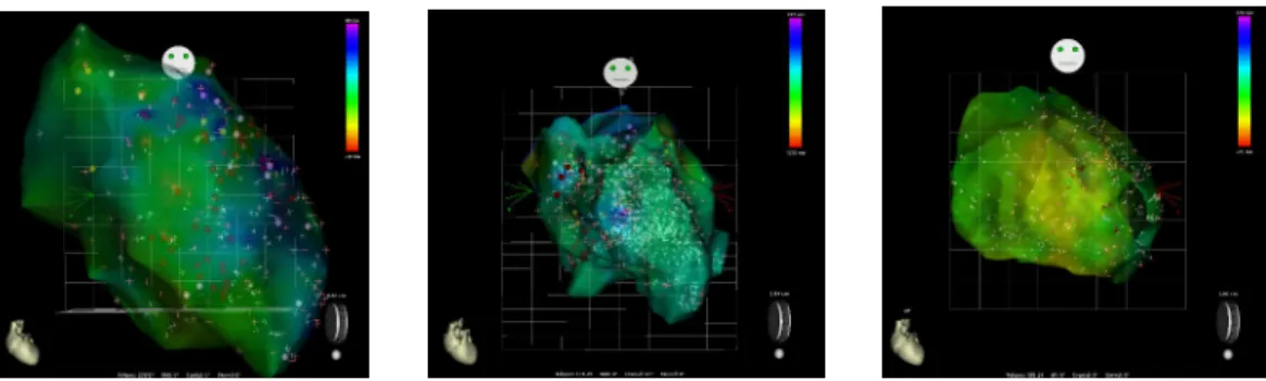
LV non-contact electroanatomic mapping (EAM) was performed using a multi-electrode array catheter (EnSite Velocity System, St Jude Medical, MN, USA) passed via the femoral artery retrogradely across the aortic valve into the LV cav-ity in all seven patients. The EnSite system uses the inverse solution method to reconstruct endocardial electrical potentials within the LV cavity [Schilling 1998]. The chamber geometry was reconstructed using locator signals from a steerable electrophysiological catheter. Three patients (Patients 1-3) with ICM underwent a simultaneous VT stimulation study according to the Wellens protocol with pacing from the RV apex during the mapping study [Wellens 1985] as part of the clinical work-up for risk stratification to determine if an ICD should be implanted as per National guidelines [Nat 2006].
Unipolar electrograms (UEG) derived from non-contact mapping were filtered from an electrophysiology recorder (EnSite Velocity System) with a band-pass filter. In order to optimize QRS complex and T wave detections, the high-pass and low-pass filter cut-off frequencies were set respectively at 10Hz/300Hz and 0.5Hz/30Hz. The data were then exported for offline analysis. The depolarization times were detected within the QRS window and derived from the zero crossings of the laplacian of the measured UEGs [Coronel 2000]. The repolarization times were detected within the ST window for the signals and derived using the alternative method [Yue 2004]. The alternative method has repolarization times derived from −dV/dtmax for the
nega-tive T-wave, at the dV/dtmin for the positive T-wave, and the mean time between
−dV /dtmax and dV/dtmin for the biphasic T-waves.
The relationship between the diastolic interval (DI) of one cardiac cycle and the APD of the subsequent cardiac cycle is described by the APD restitution curve (APD-RC). The difference between the depolarization time and repolarization time was used to estimate the activation recovery time (ARI), which is a surrogate marker for APD. The APD-RC was estimated during steady state RV pacing (600ms, 500ms and 400ms) with sensed extras at different coupling intervals. The APD-RC was rep-resented by a non-linear equation using a least-squares fit to the mono-exponential function as previously detailed on experimental and clinical data [Relan 2011a]
[Relan 2011b]: a single APD-RC was fitted for each measured point from the EAM
and the maximum APD was estimated as the asymptotic APD of the APD-RC, when the DI tends to infinity.
3.2.4 Cardiac Electrophysiology Models
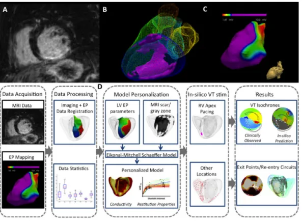
The present study used a coupled personalization framework that was previously evaluated in details [Relan 2011a] [Relan 2011b]. It combines the benefits of two different kinds of mathematical models while keeping the computational complexity tractable. The Eikonal (EK) model was used to estimate the conductivity parame-ters over the ventricle derived from non-contact mapping of the ventricular endocar-dial surface potential, which were then used to set the parameters for the Mitchell-Schaeffer (MS) model. Additionally, the MS model is able to hold the memory of one preceding cycle and has restitution properties, thus is able to simulate arrhythmias macroscopically. Both models are computed on the whole 3D myocardium. This personalization framework has already been detailed in a previous publication and the predictive power of such personalized model was evaluated on experimental data
[Relan 2011a] [Relan 2011b]. The process of building the models from the MRI and
EAM data is illustrated in Figure3.1and a summary on the used models and their personalization are included in the following sections.
Figure 3.1: Personalized computer modelling process. Upper panel: (A) high-resolution contrast-enhanced MRI scar images; (B) whole heart model segmented from 3D steady-state free precession (SSFP) MRI with scar (core and gray zone) in violet; (C) low voltage areas from electroanatomical mapping. Lower panel: (D) model personalization and in silico VT stimulation study procedure workflow.