Bubbles and self-fulfilling crises

HAL Id: halshs-00590568

https://halshs.archives-ouvertes.fr/halshs-00590568

Preprint submitted on 3 May 2011

HAL is a multi-disciplinary open access

archive for the deposit and dissemination of sci-entific research documents, whether they are pub-lished or not. The documents may come from teaching and research institutions in France or abroad, or from public or private research centers.

L’archive ouverte pluridisciplinaire HAL, est destinée au dépôt et à la diffusion de documents scientifiques de niveau recherche, publiés ou non, émanant des établissements d’enseignement et de recherche français ou étrangers, des laboratoires publics ou privés.

Bubbles and self-fulfilling crises

Edouard Challe, Xavier Ragot

To cite this version:

P

ARIS

-J

OURDAN

S

CIENCES

E

CONOMIQUES

48, BD JOURDAN – E.N.S. – 75014 PARIS TEL. : 33(0) 1 43 13 63 00 – FAX : 33 (0) 1 43 13 63 10

www.pse.ens.fr

WORKING PAPER N° 2005 - 44

Bubbles and self-fulfilling crises

Edouard Challe Xavier Ragot

JEL Codes : G12, G33

Keywords : Credit market imperfections, self-fulfilling expectations, financial crises.

Bubbles and Self-ful…lling Crises

Edouard Challe

CNRS-CEREG, University of Paris-Dauphine,

Place du Maréchal de Lattre de Tassigny, 75116 Paris, France

Email: edouard.challe@dauphine.fr

Tel: +33 (0)1 44 05 45 65

Fax: +33 (0)1 44 05 40 23

(corresponding author)

Xavier Ragot

CNRS-PSE, 48 bd Jourdan 75014 Paris, France

Email: ragot@pse.ens.fr

Tel : +33 (0)1 43 13 63 04

Fax : +33 (0)1 43 13 63 10

February 20, 2007

We received helpful feedback from seminar participants at the University of Cambridge, Paris-Jourdan Sciences Economiques, the University of Paris-Dauphine and the University of Paris X-Nanterre, as well as from conference participants at the Paris Finance International Meeting (Paris, December 2005), the Theory and Methods of Macroeconomics Conference (Toulouse, January 2006), and the Society for Economic Dynamics Conference (Vancouver, July 2006). We are particularly grateful to Jean-Pascal Benassy and Gilles Chemla for their comments and suggestions. All remaining errors are ours.

Abstract: Financial crises are often associated with an endogenous credit reversal, followed by a fall in asset prices and serious disruptions in the …nancial sector. To account for this sequence of events, this paper constructs a model where excessive risk-taking by investors leads to a bubble in asset prices, and where the supply of credit to these investors is endoge-nous. We show that the interplay between excessive risk-taking and the endogeneity of credit may give rise to multiple equilibria associated with di¤erent levels of lending, asset prices, and output. Stochastic equilibria lead, with positive probability, to an ine¢ cient liquidity dry-up, a market crash, and widespread failures by borrowers. The possibility of multiple equilibria and self-ful…lling crises is shown to be related to the severity of the risk-shifting problem in the economy.

Keywords: Credit market imperfections; self-ful…lling expectations; …nancial crises. JEL codes: G12; G33.

1

Introduction

The resurgence of …nancial crises over the past twenty years, both in OECD and developing countries, has sparked renewed interest in the potential sources of …nancial fragility and market imperfections from which they originate. Although each crisis had, of course, its own particular features, it is now widely agreed that many of them were characterised by a common underlying pattern of destabilising developments in credit and asset markets. Amongst OECD countries in the 1980s and early 1990s, such as Japan or the Scandinavian countries, …nancial crises were an integral part of a broader ‘credit cycle’whereby …nancial deregulation led to an increase in available credit, fuelled a period of overinvestment in real estate and stock markets, and led to high asset-price in‡ation. These events were then followed by a credit contraction (or ‘crunch’) and the bursting of the asset bubble, causing the actual or near bankruptcy of the …nancial institutions which had initially levered the asset investment1_{. A similar sequence of events has been observed in a number of Asian} and Latin American countries, where capital account liberalisation allowed large amounts of capital to ‡ow in during the 1990s, with a similar e¤ect of raising asset prices to unsustainable levels. This phase of overlending often ended in a brutal capital account reversal followed by a market crash and a banking crisis.2

An important theoretical issue, as yet largely unanswered, is whether the credit turn-around that typically accompanies …nancial crises is the outcome of an autonomous, ‘extrin-sic’, reversal of expectations on the part of economic agents, or simply the natural outcome of accumulated macroeconomic imbalances or policy mistakes, i.e., the intrinsic fundamen-tals of the economy. For a time, the consensus was to interpret crises simply as the outcome of extraneous ‘sunspots’ hitting the beliefs of investors, regardless of the underlying fun-damental soundness of the economy. For example, early models of crises would emphasise the inherent instability of the banking system, whose provision of liquidity insurance made banks sensitive to self-ful…lling runs, as the ultimate source of vulnerability to crises3. In a similar vein, ‘second-generation’ models of currency crises would insist on the potential

1_{See Borio, Kennedy and Prowse (1994) and Allen and Gale (1999, 2000), as well as the references therein,}

for a more detailed account of these events.

2_{See Calvo (1998), Kaminsky (1999) and Kaminsky and Rheinart (1998, 1999) for the evidence on this}

sequence of events, often referred to as ‘sudden stop’.

existence of multiple equilibria in models of exchange rate determination, where the defense of a pre-announced peg by the central bank is too costly to be fully credible4.

Although such expectational factors certainly play a rôle in triggering …nancial crises, theories based purely on self-ful…lling expectations clearly do not tell the full story. In virtually all the recent episodes brie‡y mentioned above, speci…c macroeconomic or structural sources of fragility preceded the actual occurrence of the crisis. In OECD countries, for example, …nancial crises usually followed periods of loose monetary policy or poor exchange-rate management (e.g., Borio et al., 1994). In emerging countries, the culprit was often to be found in the weakness of the banking sector, due to poor …nancial regulation, as well as other factors such as unsustainable …scal or exchange rate policies (Summers, 2000). Overall, the evidence from this latter group of countries indicates that factors of fundamental weakness explain only some of the probability of a crisis, suggesting that both fundamental and non-fundamental elements are at work in triggering …nancial crises (see Kaminsky, 1999, and the discussion in Chari and Kehoe, 2003).

The model of …nancial crises that we develop below aims to account for both the credit-asset price cycle typical of recent crises and the joint role of fundamental and nonfundametal factors in making crises possible. In so doing, we draw on Allen and Gale (2000), for whom …nancial crises are the natural outcome of credit relations where portfolio investors borrow to buy risky assets, and are protected against bad payo¤ outcomes by the use of debt contracts with limited liability. Investors’ distorted incentives then lead them to overinvest in risky assets (i.e., a risk-shifting problem arises), whose price consequently rises to high levels (leading to an asset bubble), with the possibility that investors go bankrupt if asset payo¤s turn out badly (a …nancial crisis occurs). Unlike Allen and Gale, however, who study the risk-shifting problem in isolation and make the partial-equilibrium assumption that the amount of funds available to investors is exogenous, we allow for endogenous variations in the supply of credit resulting from lenders’ utility-maximising behaviour. We regard this alternative speci…cation as not only more realistic, but also particularly relevant to our understanding of recent crises episodes, where the endogeneity of aggregate credit was frequently identi…ed as being an important source of …nancial instability5_.

Our results indicate that the interdependence between excessive risk-taking by investors

4_{E.g., Obsfeld (1996) and Velasco (1996).}

and the elasticity of aggregate credit is indeed a serious factor of endogenous instability. First, we show that, under risk-shifting, the equilibrium return that lenders expect from lending to investors may be non-monotonic and increase with the aggregate quantity of loans, rather than decrease, as standard marginal productivity arguments would suggest. The explanation is that investors’ optimal portfolio composition typically changes as the amount of funds that is lent to them varies, i.e., the ‘assets’and ‘liabilities’sides of investors’ balance-sheets are not independent. In certain circumstances, which we derive and explain in the paper, an increase in investors’ liabilities may increase the share of safe assets in their portfolios, which tends to raise the ex ante return on loans. When strong enough, this ‘portfolio composition’e¤ect may dominate the usual ‘marginal productivity’e¤ect, so that the expected return on loans increases with aggregate loans (for some range of total loans at least). This strategic complementarity naturally leads to the existence of multiple equilibria associated with di¤erent levels of aggregate lending, asset prices, and output. We relate the intensity of these strategic complementarities, and the resulting possibility of multiple equilibria, to the severity of the risk-shifting problem in the economy.

We then consider the case where multiple equilibria do exist, and where the selection of an equilibrium with low lending follows a ‘sunspot’, i.e., an extraneous signal of any ex ante probability on which agents coordinate their expectations. We show that such stochastic equilibria generate self-ful…lling crises with the following characteristics; i) lending to portfolio investors drops o¤ as lenders choose to consume or store, rather than lend, a large share of their endowment (credit contraction), ii) this causes a fall in investors’ resources and a drop in their demand for …xed-supply assets, whose price consequently falls to low levels (market crash), and iii) this fall in prices forces into bankruptcy investors who had previously borrowed to buy assets, as the new value of their assets falls short of their liabilities (…nancial sector disruptions). In short, weak fundamentals make multiple equilibria possible, while self-ful…lling expectations trigger the actual occurrence of the crisis. We also provide a full welfare analysis of the model. Crises are shown to unambiguously decrease ex ante welfare, with a principal source of this welfare loss being the negative wealth e¤ects of the crash on lenders’consumption levels.

Although our theory of …nancial crises draws on recent related contributions, it also di¤ers from them in several dimensions. While Allen and Gale (2000) and Edison et al. (2000)

both emphasise the interdepency between asset price movements and aggregate credit during crises, they do so in the framework of single-equilibrium models where crises are entirely explained by exogenous fundamentals. Building on the empirical results of Kaminsky (1999) discussed above, Chari and Kehoe (2003) account for the probability of crises unexplained by fundamental factors by relying on investors’ ‘herd behaviour’ in an environment with heterogenous information; in contrast, our results are derived within a rational expectations framework where all investors share the same information about asset payo¤s. Finally, within the class of multiple-equilibrium based theories, our framework di¤ers from ‘third generation’ models of currency crises (e.g., Aghion, Bacchetta and Banerjee, 2001 and 2004) by focusing on the instability of aggregate credit, rather than the volatility of nominal exchange rates; it also di¤ers from in…nite-horizon models where self-ful…lling asset-price movements are the outcome of ‘steady state indeterminacy’, i.e., the multiplicity of converging perfect-foresight equilibrium paths (as in Challe, 2004, for example).6

The remainder of the paper is organised as follows. Section 2 introduces the model and derives its unique fundamental (i.e., …rst-best e¢ cient) equilibrium. Section 3 shows how the interdependency between endogenous lending and the excessive risk-taking of portfolio investors may give rise to multiple equilibria associated with di¤erent levels of lending, asset prices, and output. Section 4 derives the stochastic equilibria of this economy (i.e., equilibria featuring self-ful…lling crises), and analyses their welfare properties. Section 5 o¤ers two extensions to the basic model, while Section 6 concludes.

2

The model

2.1

Timing and assets

There are three dates, 0, 1 and 2, and two real assets. One asset, safe and in variable supply, is two-period lived and yields f (x) units of the (all-purpose) good at date t+1 for x 0units invested at date t; t = 0; 1. It is assumed that f (:) is a twice continuously di¤erentiable

6_{Caballero and Krishnamurthy (2006) o¤er a model of emerging country bubbles where the bursting of}

the bubble is associated with a capital ‡ow reversal. In their model, the existence of bubbles is related to the relative scarcity of available stores of value (as in Tirole (1985)), while our bubbles owe their existence to agency problems in the …nancial sector leading to excessive risk-taking by investors.

function satisfying f0_{(x) > 0; f}00_{(x) < 0; f (0) = 0; f}0_{(0) = 1 and f}0_{(1) = 0. Moreover,} the following standard assumption is made to limit the curvature of f (:), for all x > 0:

(x) xf00(x) =f0(x) < 1: (1)

The other asset is risky, in …xed supply (normalised to 1), and three-period lived –it is available for buying at date 0 and delivers a terminal payo¤ R at date 2, where R is a random variable at dates 0 and 1 that takes on the value Rh with probability _{2 (0; 1] ; and} 0otherwise, at date 2. Although more general distributions for the fundamental uncertainty a¤ecting the asset payo¤ can be considered, we choose this simple speci…cation in order to focus on the extrinsic uncertainty generated by the presence of multiple equilibria.

The interpretation of this menu of available assets is that the supply of the risky asset responds slowly to changes in its demand (think of real estate, for example), while that of the safe asset adjusts quickly, and we consider the way markets clear in the short run. The market price of the risky asset at date t, in terms of the good (which is taken as the numeraire), is denoted Pt; t = 0; 1.

2.2

Agents and market structure

The economy consists of four types of risk-neutral agents in large numbers7_{. There is a} continuum of three-period lived lenders of mass 1, who enter the market at date 0 and leave it at date 2. Their intertemporal utility is u (c1; c2) = c1 + c2, where ct; t = 1; 2, is date t consumption and > 0 is the discount factor (lenders do not enjoy date 0 consumption). Lenders receive an endowment e0 > 0 at date 0 and e1 at date 1, regarding which the following technical assumption is made:

e1 > f0 1(1= ) + Rh: (2)

As will become clear below, condition (2) is necessary and su¢ cient for all the equilibria that we analyse in the paper to correspond to interior solutions (i.e., where both c1 and c2 are positive). Given the lenders’assumed utility function, the entire endowment e0 is saved at date 0 (provided that the ex ante return on saving at date 0 is non negative, as will

7_{The paper focuses on the neutral case, in which all results can be derived analytically. The}

always be the case), while savings decisions at date 1 depend on the comparison between the expected return on savings then and the gross rate of time preference, 1= . This possibility that lenders consume, rather than lend, part of their wealth at date 1 renders aggregate lending endogenous at that date, and is the novel and crucial feature of our model.

Lenders face overlapping generations of two-period lived investors and entrepreneurs with positive mass, entering the economy at dates 0 and 1 and maximising end-of-life consumption. In the remainder of the paper, we shall refer to ‘date t investors (entrepreneurs)’ as the investors (entrepreneurs) who enter the economy at date t, t = 0; 1, and leave it at date t + 1. Neither investors nor entrepreneurs receive any endowment. Finally, the stock of risky assets is initially held by a class of one-period lived initial asset holders, who sell them to investors at date 0 and then leave the market.

There is market segmentation (i.e., restrictions on agents’ asset holdings) in the two following senses. First, only entrepreneurs have access to the production technology f (:). Since they have no wealth of their own, they borrow funds by issuing XSt corporate bonds (at the normalised price 1) at date t (= 0; 1). Entrepreneurs’ utility maximisation under perfect competition then ensures that the gross interest rate on corporate bonds at date t (= 0; 1), called rt, is equal to the marginal product of capital at the same date, f0(XSt).

Second, lenders cannot directly buy risky assets or corporate bonds, and must thus lend to investors to …nance future consumption. This restriction implies that market equilibria at dates 0 and 1 are intermediated, with lenders …rst entrusting investors with their savings, and investors then lending to entrepreneurs (i.e., buying XSt corporate bonds at price 1) and investing in risky assets (i.e., buying XRt assets at price Pt)8. We denote Bt, t = 0; 1; the demand for loans by date t investors (which, in equilibrium, equals lenders’savings at the same date). Finally, we follow Allen and Gale (2000) in assuming that lenders and investors are restricted to simple debt contracts, where the contracted rate on these loans, denoted rl

t; t = 0; 1, cannot be conditional on the loan size or, due to asymmetric information, the investor’s portfolio. As will be shown below, the use of debt contracts with limited liability causes lenders’and investors’incentives to be misaligned, and is the basic market imperfection in the model.

8_{This structure implies that lenders have no choice but to lend to investors to …nance future consumption.}

Section 5.1 shows that all our results carry over when lenders have access to a storage technology whose positive gross return competes with risky lending.

2.3

Fundamental equilibrium

In the intermediated economy described above, investors are granted exclusive access to the markets for risky assets and corporate bonds. Before analysing the resulting market outcome in more detail, it is useful to …rst derive the equilibrium that would prevail without these restrictions, i.e., if lenders could directly buy both real assets. The corresponding ‘fundamental’equilibrium, in which prices and quantities are …rst-best e¢ cient, will provide a natural benchmark against which the intermediated equilibrium can be compared. As is usual with …nite horizon economies, we work out equilibrium prices and quantities backwards, using date 1 outcomes to solve for date 0 equilibrium conditions.

Subgame equilibrium at date 1. Given their date 1 wealth, denoted W1, lenders maximise E1u (c1; c2) = c1+ E1c2. Since lenders’date 1 savings, B1, equal safe asset investment, XS1, plus risky asset investment, XR1P1, lenders’expected utility from saving B1 and choosing a portfolio (XS1; XR1) at date 1 is

W1 B1 + E1 r1FXS1+ RXR1 = W1 B1+ r1FB1+ XR1 Rh rF1P F

1 ; (3)

where P1F and rF1 denote the date 1 fundamental values of the risky asset and the interest rate, respectively. Given B1, the price of the asset in the fundamental equilibrium must be:

P₁F = Rh=r₁F: (4)

If the fundamental value of the risky assets were lower than Rh_=rF

1;then the net return on trading them, Rh rF₁P₁F; would be positive for all positive values of XR1 and lenders would want to buy an in…nite quantity of risky assets; if it were higher than Rh_=rF

1, then this net return would be negative and the demand for risky assets would be zero. Since the risky asset is in positive and …nite supply, neither PF

1 < Rh=rF1 nor P1F > Rh=rF1 can be equilibrium situations.

Using equation (4) and the fact that in equilibrium XR1 = 1 and thus r1F = f0(XS1) = f0(B1 P1F), market-clearing for corporate bonds implies:

f0 1(r₁F) + Rh=rF₁ = B1: (5)

Given the properties of f (:), equation (5) de…nes r1F uniquely for all positive values of B1. It can thus be inverted to yield the interest rate function rF1 (B1), where rF1 (B1) is continuous, strictly decreasing, and such that r1F(0) =1 and r1F(1) = 0.

Substituting (4) into (3), we can see that lenders’expected utility is W1 B1+ B1rF1 (B1). Given lenders’utility functions and our assumption of a high enough date 1 endowment (see (2)), lenders increase savings up to the point where the rate of return on savings, rF

1 (B1) ;is equal to the gross rate of time preference, 1= (see …gure 1 below). Substituting rF

1 = 1=

into equations (4) and (5), we …nd that asset prices and aggregate savings in the fundamental equilibrium are uniquely determined and given by:

P₁F = Rh; (6)

B₁F = f0 1(1= ) + Rh; (7)

where inequality (2) ensures that B1F < e1;i.e., that the fundamental equilibrium is interior. In short, lenders’risk neutrality implies that the fundamental value of the asset, PF

1 , is equal to the discounted expected dividend stream, Rh; while capital investment, XS1F ; is at the point where its rate of return equals lenders’rate of time preference, f0 1_{(1= ).}

Equilibrium at date 0. The fundamental price vector at date 1, (PF

1 ; rF1); can now be used to derive that at date 0, (PF

0 ; rF0), by simply noting that the equilibrium price of risky assets at date 1, PF

1 ; is also the payo¤ from holding them from date 0 to date 1. Lenders’ total (deterministic) payo¤ at date 1 from choosing a portfolio (XS0; XR0) at date 0 is then rF0X0S+ PF

1 XR0, which they maximise subject to the portfolio choice constraint XS0+ P0FXR0 = e0, while taking r0 and P0 as given. They thus maximise:

rF₀X0S + P1FXR0 = e0rF0 + XR0 P1F r F 0P

F

0 :

Given e0r0F, the fundamental value of the risky asset at date 0 cannot be higher (lower) than PF

1 =rF0, since asset demand would then be equal to zero (in…nity). It must thus be:

P₀F = P₁F=r₀F = Rh=rF₀: (8)

Using (8), the properties of f (:), and the fact that XR0 = 1 and thus rF0 = f0(XS0) = f0_(e

0 P0F) in equilibrium, r0F is uniquely determined by the following equation:

f0 1(rF₀) + Rh=rF₀ = e0: (9)

Equations (8)–(9) fully characterise equilibrium prices and quantities at date 0 and com-plete our derivation of the fundamental equilibrium of this economy. The remainder of the paper then works out equilibrium prices and quantities for the intermediated case, i.e., where lenders no longer have direct access to the markets for risky assets and corporate bonds.

3

Endogenous lending and multiple equilibria

This Section and the following one derive the intermediated equilibrium (equilibria) of the economy, using a method similar to that used for the fundamental case above. The present Section solves for the equilibrium at date 1, and shows how the interplay between endogenous lending and the risk-shifting problem may lead to multiple equilibria. Section 4 then uses date 1 outcomes to derive the stochastic equilibria of the full model.

3.1

Market clearing at date 1

Contracted loan rate. Date 1 investors borrow B1 ( 0)from lenders, which they use to buy XS1corporate bonds at price 1 and XR1 risky assets at price P1 (so that B1 = XS1+ XR1P1). The use of debt contracts with limited liability allows investors to default, and earn 0, when their total payo¤ at date 2, r1XS1+ RXR1; is less than the amount owed to lenders, r1lB1. Thus, the terminal consumption of date 1 investors is:

max r1XS1+ RXR1 r1lB1; 0 = max XR1(R r1P1) + B1 r1 rl1 ; 0 :

Note from the latter equation that the contracted rate on loans between lenders and investors, rl

1, must be equal to the interest rate on corporate bonds, r1. If r1 > rl1, then investors would want to borrow an unlimited amount of funds from lenders and use them to buy corporate bonds; they would then reach the …nite limit of available funds, and from then compete for loans until r1 = rl1. If r1 < rl1then investors’loan demand would be nil, implying that the return on corporate bonds would be r1 = f0(0) = 1; a contradiction. Thus, any equilibrium in the markets for loans and corporate bonds must satisfy rl

1 = r1 = f0(XS1). At this loan rate, perfect competition amongst investors drives down the net return on trading corporate bonds to zero.

Asset prices and interest rate. Since B1 r1 r1l = 0; investors’ terminal consumption is simply max [XR1(R r1P1) ; 0] :Because XR1(0 r1P1) < 0for all P1 > 0;investors default on loans when the asset payo¤ is 0, and this occurs with probability 1 . Their expected date 2 consumption is thus XR1 Rh r1P1 , provided they do not default when the asset payo¤ is Rh _{(i.e., provided X}

R1 Rh r1P1 is non-negative, as is always the case in equilibrium). Given their objective of maximising expected terminal consumption, market clearing for the

risky asset implies that its equilibrium price must be:

P1 = Rh=r1: (10)

If the price of the asset were lower (higher) than Rh_=r

1; then Rh r1P1 would be pos-itive (negative) for all pospos-itive values of XR1 and date 1 investors would want to buy

in-…nitely many (zero) risky assets. Given (10), investors’ consumption when R = Rh _is

XR1 Rh r1P1 = 0. The reason for this is intuitive: because markets are competitive, investors must make zero expected pro…ts on trading risky assets. Since they earn zero when R = 0 and they default, they must also earn zero when R = Rh, which is ensured by the equilibrium price (10). Thus, in equilibrium the terminal consumption of date 1 investors is zero under both possible values of R at date 2.

Using equation (10) and the fact that in equilibrium XR1= 1 and r1 = f0(XS1) ;we have r1 = f0(B1 P1). Market clearing for corporate bonds at date 1 then implies:

f0 1(r1) + Rh=r1 = B1: (11)

From the hypothesised properties of f (:) ; equation (11) uniquely de…nes the equilibrium interest rate for all positive values of B1: The implied interest rate function, r1(B1) ; is continuous and such that r01(B1) < 0, r1(0) =1 and r1(1) = 0. Equations (10)–(11) then fully characterise the intermediated equilibrium price vector at date 1, (P1; r1); conditional on the amount of aggregate lending, B1.

Note from (5) and (11) that, for a given quantity of savings B1, the intermediated interest rate, r1, is higher than its fundamental analogue, r1F. This can be explained as follows. For a given value of B1; the expected asset payo¤ that accrues to investors in the intermediated equilibrium, Rh, is higher than the expected payo¤ to lenders in the fundamental equilibrium, Rh_{. In consequence, risky assets are bid up in the intermediated equilibrium and safe} asset investment, XS1; is crowded out, which in turn raises the equilibrium interest rate, r1 (relative to the fundamental rate, rF

1). The intermediated equilibrium is thus characterised by risk shifting, in the sense that portfolio delegation to debt-…nanced investors leads to an excessive share of risky asset investment, and too little safe asset investment, relative to the e¢ cient portfolio (i.e., the fundamental equilibrium). The implications of this distortion for equilibrium asset prices and savings are analysed further in Section 3.4.

3.2

Expected return on loans

Given lenders’utility functions, individual lending decisions at date 1 depend on the expected return on the loans they make to investors, denoted 1;as compared to the gross rate of time preference, 1= . Note that ₁ in general di¤ers from the contracted loan rate, r1, because of the possibility that date 1 investors default on loans at date 2.

When date 1 investors do not default on loans (i.e., when R = Rh_{), the contracted}

loan rate applies and they repay lenders r1B1. When they do default, lenders gather the residual value of investors’portfolio, i.e., the capitalised value of corporate bonds, r1XS1 = r1(B1 P1) :The ex ante unit loan return is thus r1+ (1 ) r1(1 P1=B1)or, using (10) and the interest rate function r1 = r1(B1),

1(B1) = r1(B1)

(1 ) Rh

B1

(> 0) : (12)

Note from equations (5), (11) and (12) that the probability that investors go bust at

date 2, 1 , indexes the distance between the contracted and actual ex ante returns on

savings, r1 and 1. When = 1the risk-shifting problem disappears since portfolio investors never default; the intermediated loan return, 1(B1) ; is then identical to the contracted loan rate, r1(B1) ; which in turn equals the fundamental return, rF1 (B1); in this case, the date 1 intermediated equilibrium is uniquely determined by equations (6)–(7). When < 1;

investors’and lenders’incentives become misaligned, and a gap (1 ) Rh_=B

1 > 0appears

between r1 and 1. Thus, 1 measures both the severity of the risk-shifting problem in

the economy (i.e., the extent to which investors take more risk than if they were playing with their own funds) and the implied distortion in the intermediated return on loans (i.e., r1 1).

To analyse the existence and properties of the intermediated equilibrium when < 1, we have to characterise the behaviour of ₁(B1) as total loans, B1; vary over (0; 1). First, note that 1(B1) is continuous and such that 1(1) = 0 and 1(0) = 1:9 Although this implies that @ ₁(B1) =@B1 must be negative somewhere, the two terms on the right-hand side of (12) indicate that, over a given interval [Ba; Bb] (0;1), the change in 1(B1)as a function of B1 is of ambiguous sign.

The …rst term of the right-hand side of (12), r1(B1), is the (decreasing) interest rate

9_That

function de…ned by equation (11): an increase in B1 raises the amount invested in the safe asset, XS1, which reduces the equilibrium interest rate, r1 = f0(XS1) ; and thus the average return on loans; this is the usual ‘marginal productivity e¤ect’of aggregate savings

on the loan return. In contrast, the second term, (1 ) Rh_=B

1; increases with B1; this latter e¤ect re‡ects the impact of the total loan amount on the average riskiness of loans as the composition of the optimal portfolio varies with B1. To analyse this second e¤ect in more detail, …rst use (11) to write the relationship between safe asset investment, XS1; and aggregate lending, B1, as follows:

B1 = XS1+ Rh=f0(XS1) : (13)

From (13) and assumption (1) regarding the concavity of f (:), it is easy to check that an increase in B1 raises both the quantity of safe assets, XS1, and the share of safe asset investment in investors’ portfolio, XS1=B1 (i.e., it lowers B1=XS1 = 1 + Rh=XS1f0(XS1)). In other words, even though an increase in B1 lowers r1 and thus raises asset prices, Rh=r1, the relative size of risky asset investment, P1=B1 = 1 XS1=B1; tends to decrease as B1 increases. This ‘portfolio composition e¤ect’ in turn limits the loss to lenders in case of investors’default and tends to raise the ex ante return on loans.

Given these two e¤ects, the crucial question is: Are there intervals of B1 over which 1(B1)may be increasing, i.e., where the portfolio composition e¤ect dominates the marginal productivity e¤ect? To get an insight into the conditions under which this is the case, solve (11) for Rh and substitute the resulting expression into (12) to obtain:

1(B1) = r1(B1) ( + (1 ) (XS1=B1)) : (14)

Both e¤ects are made explicit in (14). Intuitively, for the increase in XS1=B1 to dominate the decrease in r1(B1)induced by a marginal increase in B1, 1 must be su¢ ciently large (i.e., the risk-shifting problem must be large enough), and r₁0 (B1) (> 0) must be not too large (i.e., the marginal productivity e¤ect must be weak enough). When this is the case, ‘strategic complementarities’ (in the sense of Cooper and John, 1988) in lending decisions appear, as a symmetric decision by other lenders to increase their loans may then lead any individual lender to do the same. Proposition 1 formally establishes the conditions for such complementarities to occur in the general case, as well as for a more speci…c class of production functions.

Proposition 1 (Strategic complementarities). The loan return curve, ₁(B1), is in-creasing in total loans, B1, provided and f00(x)are not too large. In the isoelastic case

where f (x) = x1 _{= (1 ),}

2 (0; 1), 1(B1) has exactly one (zero) increasing interval if 2 +p < ( ) 1:

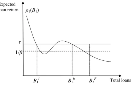
The proof is in the Appendix. For a general function f (:), there may be several intervals of B1 over which 1(B1)is increasing, i.e., over which the implied f00(XS1)is su¢ ciently small (provided is not too large). In the isoelastic case, a high value of increases the curvature of f (:) and strengthens the marginal productivity e¤ect; thus, neither nor must be too large for the portfolio composition e¤ect to dominate the marginal productivity e¤ect. In the remainder of the paper, we shall focus on a particularly simple case of non-monotonicity by assuming that ₁(B1) has one single increasing interval, as depicted in Figure 1, and as implied by the isoelastic case when 2 +p < 1(all of our results generalise straightforwardly to the case of multiple increasing intervals).

Figure 1: Loan market equilibrium at date 1

ρ

(B

)

1/β

e

B

B

B

r

(B

)

3.3

Loan market equilibrium

Having characterised the ex ante loan return, 1, as a function of aggregate loans, B1, we may now analyse the way the latter is determined in equilibrium. At date 1, lenders choose the

individual level of loans, ^B1, that maximises expected utility, c1+ E1c2;taking 1 = 1(B1) as given. Given the lenders’utility function, they …nd it worthwhile to increase (decrease) savings whenever ₁ > (<) 1= . Any interior equilibrium must thus satisfy ₁ = 1= . We focus on symmetric Nash equilibria, where consumption/savings plans are identical across lenders (i.e., ^B1 = B1) and no lender …nds it worthwhile to individually alter his own plan.

Figure 1 shows how multiple intersections between the 1(B)-curve and the 1= -line,

when they occur, give rise to multiple equilibria.10 _Bl

1 and Bh1 represent two stable levels of aggregate lending, i.e., where a symmetric marginal move away from equilibrium by all lenders alters the loan return in such a way as to move the economy back to equilibrium. The value of B1 where the 1(B1)-curve crosses the 1= -line from below is not stable and will not be discussed any further (starting from this point, an arbitrarily small increase (decrease) in B1 tends to increase (decrease) 1(B1), triggering a further move away from equilibrium). In both stable equilibria the ex ante return on loans is 1= , and lenders (expected) date 2 consumption, conditional on the selection of equilibrium j, j = l; h, is 1(B1)Bj1 = B

j 1= . Recall from equation (13) that an increase in B1 lowers marginal productivity but also reduces the share of risky assets in investors’ portfolios. The low-lending equilibrium is thus characterised by a high safe return but a high share of risky assets in the portfolio, while the high-lending equilibrium exhibits a low safe return but a safer average portfolio. Finally, notice that even though both equilibria yield the same ex ante return on loans, 1= , they are always associated with di¤erent levels of interest rates, asset prices, productive investment, and (expected) date 2 output: equation (11) and the fact that Bh

1 > B1l implies that r1(Bh) < r1(Bl): Then, denoting P1j the asset’s price, X

j

S1 productive investment, and E1( Yj j) expected date 2 output (in the sense of the total quantity of goods available for agents’consumption) when total lending is B1j, we have:

P₁h = Rh=r1(Bh) > P1l = R h_=r 1(Bl); X_S1h = f0 1 r1(Bh) > XS1l = f0 1 r1(Bl) ; E1( Yj h) = f(XS1h ) + R h _{> E} 1( Yj l) = f(XS1l ) + R h_:

10_{Assumption (2), together with the fact (as proved and analysed further in Section 3.4) that B}h 1 < B

f 1,

ensures that both B1l and B1h are interior solutions which are independent of the amount of goods that

lenders receive from the loans they made at date 0. Any income from these loans is thus consumed at date 1 (the e¤ects of date 0 loans on lenders’date 1 wealth and consumption are analysed in Section 4 2).

In short, the selection of the low-lending equilibrium raises the interest rate and depresses asset prices, productive investment, and future output, relative to the equilibrium with high lending. (More generally, there may be more than two stable equilibria if ₁(B1) has more than one increasing interval, but their properties are similar to the 2-equilibrium case, i.e., the higher is B1, the lower is r1(B1), and the higher are P1, XS1 and E1(Y )).

3.4

Comparison with the fundamental equilibrium

We emphasised above that the risk-shifting problem arising under market segmentation leads investors to overinvest in risky assets, relative to the fundamental equilibrium. Proposition 2 summarises the implications of this distortion for the price of the risky asset and the amount of aggregate saving in equilibrium.

Proposition 2 (Asset bubbles and crowding out). In both intermediated equilibria,

asset prices are higher than in the fundamental equilibrium (i.e., P₁j > PF

1 ; j = l; h), while aggregate savings are lower than in the fundamental equilibrium (i.e., B1j < B1F; j = l; h).

The proof is in the Appendix. That P₁j > PF

1 ; j = l; h; indicates that assets are overpriced at date 1 in both intermediated equilibria, i.e., both equilibria are associated with a positive bubble in asset prices (the bubble being larger, the larger is aggregate credit). Because investors are protected against a bad value of the asset payo¤ by the use of simple debt contracts, they bid up the asset, with the consequence of raising its price and its share in equilibrium portfolios (relative to the fundamental equilibrium).

The reason why savings are lower in both intermediated equilibria than in the fundamen-tal equilibrium (i.e., B1l < Bh1 < B1F) follows naturally: excessive risky asset investment by portfolio investors implies that, for any given level of savings B1, the intermediated ex ante loan return, 1(B1), is lower than the fundamental return, rF1 (B1) = 1= (see our analysis in Section 3.1). Lenders thus optimally reduce lending in the intermediated equilibrium (rel-ative to the fundamental one) up to the point where this intermediated return equals the fundamental return, i.e., the gross rate of time preference 1= . Note, as a consequence, that a double crowding out e¤ect is in fact at work on XS1in the intermediated equilibrium. First, for a given level of aggregate savings B1, bubbly asset prices crowd out safe asset investment, XS1, which raises the equilibrium interest rate, r1 = f0(XS1). Second, lenders’optimal

re-action to the resulting price distortion is to reduce savings, B1, which lowers XS1(and raises r1) even further. The crowding out of productive investment by the asset bubble is the basic source of output loss in the intermediated economy, relative to the fundamental equilibrium. The implications of this loss as to the welfare ranking of the (many) intermediated equilibria are analysed in the context of the full stochastic model below.

4

Self-ful…lling …nancial crises

The previous Section showed that the excessive risk taking of portfolio investors may lead, under endogenous credit, to the existence of multiple equilibria at date 1 associated with di¤erent levels of aggregate lending, interest rates, and asset prices. We now analyse the full time span of the model to demonstrate the possibility of a self-ful…lling …nancial crisis associated with the risk that the low-lending equilibrium is selected.

4.1

Market clearing at date 0

Crisis equilibria are constructed by randomising over the two possible lending equilibria that may prevail at date 1. More speci…cally, assume that, from the point of view of date 0, high lending is selected with probability p 2 (0; 1) at date 1, so that the ‘sunspot’ on which agents coordinate their expectations causes lending and asset prices to drop down to low levels with probability 1 p. With this speci…cation for extraneous uncertainty at the intermediate date, the model potentially has a continuum of stochastic equilibria indexed by the ex ante probability of a market crash, 1 p. Since the asset’s price at date 1 is the asset payo¤ accruing to date 0 investors, this uncertainty about asset prices creates a risk-shifting problem at date 0 similar to that created at date 1 by intrinsic uncertainty about the terminal payo¤ of the asset. This causes the asset to be bid up at date 0, with the possibility that a self-ful…lling crisis (i.e., a drop in asset prices forcing date 0 investors into bankruptcy) occurs at date 1 if the low lending/low asset prices equilibrium is selected at that date.11

11_{For the sake of conciseness, we focus on equilibria where …nancial crises may actually occur at date 1}

(i.e., where date 0 investors may go bankrupt), and thus leave out of the analysis equilibria with deterministic date 1 outcomes, i.e., p = 1 (high lending is selected for sure) and p = 0 (low lending for sure).

Contracted loan rate. Denote (P0, r0) the equilibrium price vector, rl0 the contracted loan rate, and (XS0; XR0) the portfolio of date 0 investors, all at date 0: Limited liability and the portfolio constraint B0 = XS0+ P0XS0 imply that investors’terminal consumption is:

max r0XS0+ P1XR0 r0lB0; 0 = max XR0(P1 r0P0) + B0 r0 r0l ; 0 ;

where, given our speci…cation for extraneous uncertainty about aggregate lending and asset prices, P1 is a random variable at date 0, taking on the value P1h with probability p (i.e., B1h is selected), and P1l otherwise (B1l is selected), at date 1. The contracted rate on loans at date 0, rl

0, must necessarily be equal to the rate on corporate bonds at the same date, r0. If the former were lower (higher) than r0, then date 0 investors would want to borrow in…nitely many (zero) units of goods and use them to buy corporate bonds, while the loan supply at date 0 is exactly e0 (the gross expected return on loans at date 0 is always non-negative, because the liquidation value of date-0 portfolios cannot be negative). Thus, any equilibrium must satisfy r0 = rl0 and B0 = e0.

Asset prices and interest rate. In the equilibria that we are considering, date 0 investors default on loans when the asset price at date 1 is Pl

1, but not when it is P1h. Since B0 r0 r0l = 0; their terminal consumption is XR0 P1h r0P0 0 with probability p, and 0 otherwise. Date 0 investors choose the level of XR0 that maximises expected con-sumption, pXR0 P1h r0P0 , while any potential solution to their decision problem must be such that they do not default on loans if the asset price at date 1 is Ph

1, but do default if it is Pl

1, i.e.,

P₁h r0P0 0; P1l r0P0 < 0: (15)

The demand for risky assets by date 0 investors, XR0; is in…nite (zero) if P1h r0P0 > 0 (< 0) : Market clearing thus requires that the equilibrium price of the risky asset be:

P0 = P1h=r0; (16)

which satis…es both inequalities in (15). Again, the interpretation of this equilibrium price is straightforward. Perfect competition for the risky asset by investors implies an asset price such that they make zero expected pro…t. Because they make zero pro…t from holding risky assets when the asset payo¤ is Pl

1 (i.e., when they default), they must also earn zero when it is P1h; this is exactly what the equilibrium price P1h=r0 ensures.

Aggregate lending from date 0 to date 1 is e0. In equilibrium we have XR0 = 1 and r0 = f0(XS0) = f0(e0 P0). Thus, r0 is uniquely determined by the following equation:

f0 1(r0) + P1h=r0 = e0; (17)

where Ph

1 = Rh=r1(B1h)is independent of e0, due to the interiority of B1h allowed by assump-tion (2). Note from (16)-(17) that the equilibrium price vector at date 0, (P0; r0), is uniquely determined and does not depend on the probability of a crisis, 1 p: as date 0 investors are protected against a bad shock to the value of their portfolio by the use of simple debt contracts, they simply disregard the lower end of the payo¤ distribution (i.e., the payo¤ Pl 1 with probability 1 p) when selecting their optimal portfolio.

Asset bubbles and crowding out. We complete this Section by showing that the risk-shifting problem due to date 1 extraneous uncertainty and the limited liability of date 0 investors causes asset prices to be overvalued at date 0, and to crowd out real investment at that date, XS0. From (8)–(9) and (16)–(17), the mispricing of risky assets at date 0 is given by:

P0 P0F = f0 1(r F

0) f0 1(r0) :

Using (9) and (17), together with the fact that Ph

1 > P1F (which was established in Proposition 2), it is easily seen that r0 > rF0. Since f0 1(:)is decreasing, P0 P0F > 0 and there is a positive asset price bubble at date 0. Note that e0 being exogenously given, the amount of crowding out caused by this bubble is simply XF

S0 XS0= P0 P0F:The implied lower level of capital investment at date 0 in turn lowers date 1 output, f (XS0), in the same way as date 2 (expected) output, f (XS1) + Rh;was lowered by the asset bubble at date 1.

4.2

The wealth e¤ect of crises

Having shown the existence of a continuum of stochastic equilibria indexed by the proba-bility of a self-ful…lling crisis, we are now in a position to study the welfare properties of these equilibria in more details. We …rst analyse the way crises a¤ect lenders’ wealth and intertemporal consumption plans, and then turn to the e¤ect of crises on other agents’utility. To see why lenders’wealth at date 1 is contingent on whether a crisis occurs at date 1 or not, we calculate how it is a¤ected by the possible default of date-0 investors. When these investors do not default, they owe lenders the capitalised value of outstanding debt at date

1, r0e0. As lenders receive an endowment e1 at date 1, their date 1 wealth if no crisis occurs is simply W1h = e1 + r0e0. When investors do default, on the contrary, lenders’ wealth at date 1 is their date 1 endowment, e1, plus the residual value of the date 0 investors’portfolio, r0X0S+ P1l. Using (17), lenders’date 1 wealth, W

j

1, conditional on whether a crisis occurs (j = l) or not (j = h), is thus given by:

W₁j = e1+ r0XS0+ P j

1; j = l; h: (18)

Obviously, the total quantity of goods available at date 1 is the same across equilibria, because initial capital investment, XS0, is uniquely determined (i.e., it does not depend on p). This quantity amounts to lenders’ date 1 endowment, e1, plus entrepreneurs’ produc-tion, f (XS0) ;the latter being shared between date 0 entrepreneurs, who gather the surplus f (XS0) r0XS0 in competitive equilibrium, and lenders, who receive r0XS0 (recall that P0 is such that date 0 investors consume zero whether P1 = P1l or P1h).12

From condition (2) and the second inequality stated in Proposition 2, we have B₁j < B₁F < W₁j, j = l; h, implying that both possible levels of wealth give rise to interior solutions for consumption-savings plans at date 1 where ₁(B₁j) = 1= . If a crisis occurs at date 1, then lenders’wealth and savings at that date are W1l and B1l; respectively, while their date 1 and (expected) date 2 consumption levels are Wl

1 B1l and B1l= , respectively; it follows that their discounted utility ‡ow from date 1 on is simply W1l B1l + B1l= = W1l. Similarly, if a crisis does not occur at date 1, then lenders’date 1 and date 2 consumption levels are W1h B1h and Bh1= , respectively, yielding a discounted utility from date 1 on of Wh

1. Weighing these possible outcomes with the probabilities that they actually occur, and then using (18), we …nd that lenders’ex ante utility (i.e., from the point of view of date 0) depends on the crisis probability, 1 p, as follows:

E0W1 = pW1h+ (1 p) W l 1 = e1+ r0XS0+ pP1h+ (1 p) P l 1:

12_{There are two equivalent ways of characterising lenders’budget sets at date 1: looking at their wealth,}

W₁j is assigned to date 1 consumption and date 1 lending, so that, using (18), W₁j = e1+ r0X0S + P1j =

cj₁+ B₁j; j = l; h; the total quantity of goods accruing to lenders at date 1 is ultimately shared between date 1 consumption, cj₁; and date 1 capital investment, X_S1j , so that e1+ r0X0S = cj1+ X

j

S1; j = l; h: Since

E0W1 is decreasing in 1 p, since P1h > P1land e1+r0XS0; P1land P1h do not depend on p. Note that it is the selection of the low-lending equilibrium itself that triggers the crisis which lowers lenders’wealth and discounted consumption ‡ow. Thus, the utility loss incurred by lenders when a crisis occurs is akin to a pure coordination failure in consumption/savings decisions –rather than an exogenously assumed destruction of value associated with the early liquidation of the long asset, as is often assumed in liquidity-based theories of …nancial crises (e.g., Diamond and Dybvig, 1983, Allen and Gale, 2000, and Chang and Velasco, 2002).

4.3

Aggregate welfare

We can now complete the welfare analysis of the model by studying the e¤ect of the ex ante crisis probability on other agents’consumption. With respect to investors, Sections 3.1 and 4.1 have established that both date 0 and date 1 investors consume zero in equilibrium, whatever the realisation of extrinsic (date 1) and fundamental (date 2) uncertainty. Investors’ ex ante welfare is thus zero in all equilibria. With respect to entrepreneurs, the terminal consumption of date-1 entrepreneurs is f (XS1) XS1f0(XS1), which is increasing in XS1. Since Xh

S1 > XS1l (see Section 3.3), their ex ante welfare, from the point of view of date 0, is

p f Xh

S1 XS1h f0 XS1h + (1 p) f XS1l XS1l f0 XS1l , which decreases with 1 p. Date 0 entrepreneurs consume f (XS0) f0(XS0) XS0, where XS0= f0 1(r0)does not depend on p. Finally, initial asset holders’consumption is just the selling price of the asset at date 0, P0, which is independent of p. In short, neither investors nor initial asset holders or date 0 entrepreneurs are a¤ected by the crisis probability. Lenders are, because the crisis reduces their asset wealth and discounted consumption ‡ow. Date 1 entrepreneurs are, because low lending reduces their surplus and terminal consumption. We summarise the main results derived from Section 4 in the following proposition.

Proposition 3 (Crises and welfare). When multiple levels of lending may prevail at date 1, the model has a continuum of stochastic equilibria indexed by the probability of a self-ful…lling crisis, 1 p_{2 (0; 1). The higher this probability, the lower is ex ante welfare.}

5

Extensions

Propositions 1-3 were derived under stark simplifying assumptions about agents’preferences and the technologies that are available to them. We now test the robustness of our results by relaxing two signi…cant hypotheses, namely, i) the absence of investment opportunities other than risky lending available to lenders, and ii) the risk-neutrality of all agents.

5.1

Storage and ‘‡ight to quality’

Our baseline model speci…cation implied that lenders’ choices at date 1 were limited to either consumption or risky lending to investors. Assume instead that lenders may protect themselves from excessive risk-taking by investors by investing part of their wealth at the safe return > 0. The latter may re‡ect the possibility for lenders to store wealth in the form of cash balances or government bonds in a closed economy; alternatively, it may be interpreted as the world interest rate faced by agents in a small, open economy. We show that the model with storage generates self-ful…lling crisis equilibria similar to those analysed in Sections 3-4, where all lenders symmetrically turn away from risky lending at date 1 to seek safer investment opportunities. In other words, a ‡ight to quality (rather than a contraction in aggregate savings) triggers the market crash and …nancial crisis.

To keep this alternative formulation of the model concise, assume that the storage tech-nology is available between dates 1 and 2 only.13 _{At date 0, lenders lend their entire date 0} wealth, e0, to investors as before. At date 1, they may now spread their current wealth, W1, between loans to investors, ^B1, storage, ^S1, and current consumption, c1 = W1 B^1 S^1. Subgame equilibrium at date 1. The problems faced by entrepreneurs and investors at date 1 are exactly the same as those in the baseline model. Consequently, they yield the same equilibrium pricing equations (10)–(11) and implied ex ante loan return function (12). Given their current wealth level W1;lenders now choose the quantities ( ^B1, ^S1) that maximise:

E1(c1+ c2) = W1 B1 S^1 + 1B^1+ S^1 ;

subject to ^B1+ ^S1 W1; and taking and 1 as given. If < 1= , then lenders will never …nd it worthwhile to store and thus choose ^S1 = 0; in which case all potential equilibria are

13_{Our results can be generalised to the situation where it is also available from date 0 to date 1, but the}

identical those analysed in Sections 2-4. We focus on the only robust interesting case by assuming:14

> 1= : (19)

When (19) holds, lenders will never …nd it worthwhile to consume at date 1 and choose c1 = 0. They thus maximise E1(c2) = 1B^1+ ^S1;subject to W1 = ^B1+ ^S1. All symmetric, interior solutions to this problem are such that ^B1 = B1 > 0; ^S1 = S1 > 0, and

1(B1) = r1(B1) (1 ) Rh=B1 = ;

where r1(B1) is de…ned by equation (11). It is easy to check that assumptions (2) and (19) imply that e1 > f0 1( ) + Rh= , which in turn ensures that every potential equilibrium is interior. Figure 2 shows how multiple intersections between the 1-curve and the -line, when they occur, give rise to multiple, symmetric Nash equilibria at date 1, associated with di¤erent levels of lending and storage. The only di¤erence with the baseline model here is that the appropriate required rate of return, against which ₁ is compared by lenders, is now

rather than 1= .

Figure 2: Loan market equilibrium with storage

Expected loan return

ρ

(B

)

1/β

B

B

τ

B

Equilibrium at date 0. Just as in the baseline model, assume that the model has two stable subgame equilibria at date 1, Bl

1 and B1h, and that, from the point of view of date 0, B1h is

14_{In the knife-edge situation where = 1= , B}

1and S1+ C1depend on which equilibrium is selected, but

selected with probability p 2 (0; 1). It is easy to check that investors’, entrepreneurs’and lenders’problems are exactly the same as those described in Section 4.1. Consequently, they yield the same price vector (P0; r0) as that implied by (16)-(17). Then, it is straightforward to show the the two statements contained in proposition 3 apply: the model with storage gen-erates a continuum of stochastic of crisis equilibria, while aggregate welfare unambiguously decreases with the probability of crisis 1 p.

5.2

Risk-averse agents

The assumption of limited investor’s liability, coupled with the hypothesis of all agents’risk neutrality, introduces a great deal of ‘risk-loving’behaviour in the economy. This naturally raises the question whether our results are still valid when agents, especially lenders, are risk-averse. To investigate this case, assume that investors and entrepreneurs maximise a utility function v (:) of terminal consumption, de…ned over (0; 1) and such that v0_{(:) > 0, v}00_{(:) 0,} while lenders’ intertemporal utility is now u (c1; c2) = c1+ v (c2). Entrepreneurs’ choices at dates 0 and 1 are not altered by this generalisation, since their terminal consumption is positive and deterministic. It is easy to check that investors’decisions are not modi…ed either, relative to the risk-neutral case, provided they receive an (arbitrarily small) extra terminal endowment ~e > 0.15 At date 1, lenders now choose individual lending, ^B1; which maximises c1+ E1v (c2) ;taking aggregate lending, B1, asset prices, P1, and the interest rate, r1, as given. If date 1 investors do not default, any individual lender having lent ^B1 receives the contractual repayment r1B^1 at date 2. If investors do default, this lender is entitled to a share of the residual portfolio, r1(B1 P1) ;proportional to his share in investors’liabilities,

^

B1=B1. Lenders thus solve: max ^ B1 W1 B^1+ v(r1B^1) + (1 ) v B^1 r1(B1 P1) B1 : (20)

Recall that lenders’date 1 wealth, W1;is state contingent, as it depends on the capitalised value of lenders’ date 0 loans (see Section 4.3). However any possible equilibrium value of

15_{The expected utility of date 1 investors is then (1 ) v (~e) + v X}

R1 Rh r1P1 + ~e ,

yield-ing the asset demand Rh _r

1P1 v0 XR1 Rh r1P1 + ~e = 0; in equilibrium XR1 = 1 and Rh

r1P1 = 0 since v0(~e) is positive and …nite. Similarly, the date 0 investors’ asset demand is such that

Ph

1 r0P0 v0 XR0 P1h r0P0 + ~e = 0, yielding (16) in equilibrium. An alternative assumption is that

~

W1 can be made large enough, by increasing e1 su¢ ciently, for all corresponding values of B1 to be interior. Assuming interiority, solving (20) for ^B1, and then using P1 = Rh=r1 and imposing symmetry across lenders ( ^B1 = B1), we …nd that any equilibrium lending level of the intermediated economy must satisfy:

(B1) r1v0(r1B1) + (1 ) r1 Rh B1 v0 r1B1 Rh = 1 ; (21)

where, from investors’optimal portfolio choice, r1 = r1(B1)is de…ned by equation (11) above. Note that when v (x) = x then (B1) = 1(B1) and (21) is reduced to 1(B1) = 1= , our equilibrium condition under risk neutrality. Thus, (:) generalises the ₁(:)function for the risk-averse case, and can consequently be interpreted as the ‘risk-corrected’ex ante return that lenders expect from their loans to investors (which is 1= in equilibrium).

Figure 3: The risk-corrected expected loan return

0,5 1,0 1,5 0,06 0,07 0,16 1,33 B1 ψ(B1) s igm a=0,0 s igm a=0,1 s igm a=0,2

The existence of multiple equilibria requires that (:) be increasing over at least one interval of B1. Since we could derive no simple analytical condition ensuring that this is the case, we computed the (B1) function numerically for the isoelastic case, where

f (x) = x1 _{= (1 ) ;}

2 (0; 1) ; and v (x) = x1 _{= (1 ) ; 0;for a variety of parameter} values. We found that (B1)may have an increasing interval if the risk-shifting problem is large enough (i.e., 1 is not too small), and if neither f (:) nor u (:) are too concave (i.e.,

neither nor are too large). We know from proposition 2 and the discussion in Section

3.2 that high values of or are detrimental to multiple equilibria because they make it

less likely that the portfolio composition e¤ect dominate the marginal productivity e¤ect; a positive value of strengthens the marginal productivity e¤ect further by making lenders less willing to substitute current consumption, c1, for future risky consumption, c2.

For sake of illustration, Figure 3 represents the risk-corrected loan return curve when = Rh = 0:1 and = 0:5;for di¤erent values of ; As gradually increases, the increasingness of (:) becomes less and less pronounced over the relevant range of B1, until (:) decreases over the entire (0; 1) interval. Since date 0 equilibrium values are not a¤ected by this generalisation, we conclude that multiple equilibria and self-ful…lling crises may still exist in the risk-averse economy, provided that lenders are not ‘too’risk averse.

6

Concluding remarks

This paper o¤ers a simple theory of self-ful…lling …nancial crises based on the excessive risk taking of debt-…nanced portfolio investors. In our model, the interplay between the amount of funds available to investors, the composition of their portfolio, and the return that they are able to o¤er in competitive equilibrium, creates a strategic complementarity between lenders’ savings decisions, which naturally give rise to multiple equilibria associated with di¤erent levels of lending, interest rates, asset prices and future output. Expectations-driven …nancial crises may then occur with positive probability as soon as the economy exhibits (at least) two possible equilibrium levels of lending, and the coordination of lenders on a particular equilibrium is determined by an extraneous ‘sunspot’. We showed that such crises are characterised by a self-ful…lling credit contraction, followed by a market crash, widespread failures of investors, and a fall in productive investment.

Apart from demonstrating that credit intermediation based on debt contracts is a poten-tial source of endogenous …nancial instability, the model also provides new insights into the potential welfare costs of …nancial crises. In our model, the dramatic reduction in lending and asset prices associated with the crisis equilibrium has two implications. First, it brings about a reduction in lenders’wealth due to a fall in the total value of their capitalised invest-ment, which reduces their discounted consumption ‡ow from the time of the crisis onwards. Second, the credit contraction associated with the crisis causes a fall in productive invest-ment and output, and consequently reduces entrepreneurs’pro…ts and consumption. Thus, both savers and …nal producers are hurt by the …nancial crisis, while intermediate investors, whose risk is hedged by the use of debt contracts, are ultimately left unharmed.

Appendix

Proof of proposition 1

From equation (12), we have that @ (B1) =@B1 > 0 if and only if r₁0 (B1) B12 < (1 ) R

h_{: (A1)}

Given and Rh_{; (A1) may hold if r}0

1(B1) is small enough over some interval of B1, that is if the interest rate, r1, is not very responsive to changes in the implied level of safe asset investment, XS1. This in turn holds if f (XS1) is ‘‡at enough’over the relevant range of XS1, so that r1 = f0(XS1) responds only little to changes in XS1. Using (11), together with the fact that @f0 1_(r

1) =@r1 = 1=f00(XS1), the left-hand side of (A1) yields:

r0₁(B1) B12 =

Rh+ XS1f0(XS1) 2

Rh_{+ f}0_(XS1)2_{= ( f}00_(XS1)) (> 0):

For XS1 2 X; X , i.e. when B1 2 X + Rh=f0(X) ; X + Rh=f0 X , r01(B1) B12 can be made gradually smaller by decreasing the curvature of f (:) over X; X ; in this case f0_(X

S1) is bounded both above and below, and f00(XS1) can be made arbitrarily small, producing a value of r₁0 (B1) B12small enough for (A1) to hold (provided 6= 1). The larger is 1 , the more likely it is that inequality (A1) is satis…ed, for a given r1(B1)function.

Consider now the isoelastic case. When f (XS1) = X 1 S1 = (1 ) ;equation (11) becomes B1(r1) = r 1= 1 + Rhr 1

1 , which in turn implies:

r₁0 (B1) = 1 B0 1(r1) = 1 ( 1= ) r₁1 1= Rh_r 2 1 ;

where r1 = r1(B1). From equation (12), @ 1(B1) =@B1 > 0 (< 0)when r01(B1)+(1 ) Rh=B12 > 0 (< 0), that is, when

1 ( 1= ) r₁1 1= Rh_r 2 1 + (1 ) =R h (r₁1= + Rh_r 1 1 )2 > 0 (< 0) :

De…ning Y r₁1 1= and rearranging, we …nd that ₁(B1) increases (decreases) when

(Y ) = Y2+ Rh 2 1 Y + Rh 2< 0 (> 0) :

The expression (Y )_{changes sign over (0; 1) if} (Y ) = 0 has two real roots, including at least one positive root. A necessary condition for this to hold is that the discriminant of

(Y ) = 0 be positive, i.e., the following inequality must hold:

1 + 4 ( 1) > : (A2)

When (A2) holds, the roots Ya, Yb of (Y ) = 0 are: Ya;b= Rh 2 0 @ 1 2 s 1 2 2 4 1 A :

Both roots are positive (negative) if 1 2 > (<) . Combined with inequality (A2), this means that (Y ) _{changes signs over (0; 1) if and only if}

2 +p < 1: (A3)

(Y )_{is negative for Y 2 (Y}a; Yb) ;and positive for Y 2 (0; Ya)[(Yb;1). Since Y = r 1 1=

1 ,

this means that (Y )is negative for intermediate values of r1 and positive otherwise. Using (11) again, this in turn implies that, provided (A3) holds, ₁(B1) is strictly increasing for intermediate values of B1 and strictly decreasing otherwise. When (A3) does not hold, then

(Y )is non-negative and ₁(B1)is decreasing or ‡at over (0; 1) :

Proof of proposition 2

Comparing equations (6) and (10), we have that P1j > P1F, j = l; h; if and only if r1(B

j

1) < 1= ; j = l; h:

In equilibrium, 1(B j

1) = 1= : Then, substituting (14) into the above inequality, we …nd that P₁j > PF

1 if and only if X j S1=B

j

1 > 0; which is always true whether j = l or h. Turning to the second inequality in this proposition, …rst use 1(B

j

1) = 1= ; together with equations (11) and (12), to rewrite B₁j as follows:

B₁j = r1(Bj1)f0 1 r1(B1j) + R

h_{; j = l; h:}

Comparing the latter equation with (7), we …nd that B₁j < BF

1 if, and only if, r1(B1j)f0 1 r1(B1j) < (1= ) f0 1(1= ) ; j = l; h:

r1f0 1(r1)falls with r1 since f0 1(r1) + r1f0 10(r1) = XS1+ f0(XS1) =f00(XS1)is negative by assumption (1). Thus, r1f0 1(r1) < (1= ) f0 1(1= )if and only if r1(B

j

1) > 1= ; j = l; h, which is necessarily true from (12) and the fact that ₁(B₁j) = 1= .

References

Allen, F. and Gale, D., 2000. Bubbles and crises. Economic Journal 110, 236-55.

Allen, F. and Gale, D., 1999. Bubbles, crises, and policy. Oxford Review of Economic Policy 15, 9-18.

Allen, F. and Gale, D., 1998. Optimal …nancial crises. Journal of Finance 53, 1245-84. Aghion, P., Bacchetta, P. and Banerjee, A., 2004. A corporate balance-sheet approach to currency crises. Journal of Economic Theory 119, 6-30.

Aghion, P., Bacchetta, P. and Banerjee, A., 2001. Currency crises and monetary policy in an economy with credit constraints. European Economic Review 45, 1121-1150.

Borio, E.V., Kennedy, N. and Prowse, S. D., 1994. Exploring aggregate asset price ‡uctua-tions across countries: Measurement, determinants and monetary policy implica‡uctua-tions. BIS Working Paper no 40, April.

Caballero, R.J. and Krishnamurthy, A., 2006. Bubbles and capital ‡ow volatility: Causes and risk management. Journal of Monetary Economics 53, 35-53.

Calvo, G.A., 1998. Capital ‡ows and capital-market crises: The simple economics of sudden stops. Journal of Applied Economics 1, 35-54.

Challe, E., 2004. Sunspots and predictable asset returns. Journal of Economic Theory 115, 182-190.

Chang, R. and Velasco, A., 2002. A model of …nancial crises in emerging markets. Quarterly Journal of Economics 116, 489-457.

Chari, V.V. and Kehoe, P.J., 2003. Hot money. Journal of Political Economy 111, 1262-92. Cooper, R. and John, A., 1988. Coordinating coordination failures in Keynesian models. Quarterly Journal of Economics 103, 441-464.

Diamond, D.W. and Dybvig, P.H., 1983. Bank runs, deposit insurance, and liquidity. Jour-nal of Political Economy 91, 401-19.

Edison, H.J., Luangaram, P. and Miller, M., 2000. Asset bubbles, leverage and ‘lifeboats’: Elements of the East Asian crisis. Economic Journal 110, 309-334.

Kaminsky, G.L., 1999. Currency and banking crises: The early warnings of distress. IMF Working Paper 99/178, December.

Kaminsky G.L. and Reinhart, C.M., 1999. The twin crises: The causes of banking and balance-of-payments problems. American Economic Review 89, 473-500.

Kaminsky G.L. and Reinhart, C.M., 1998. Financial crises in Asia and Latin America: Then and now. American Economic Review 88, 444-448.

Obstfeld, M., 1996. Models of currency crises with self-ful…lling features. European Eco-nomic Review 40, 1037-1047.

Summers, L.H., 2000. International …nancial crisis: Causes, prevention, and cures. American Economic Review 90, 1-16.

Tirole, J., 1985. Asset bubbles and overlapping generations. Econometrica 53, 1499-1528. Velasco, A., 1996. Fixed exchange rates: Credibility, ‡exibility and multiplicity. European Economic Review 40, 1023-1035.