HAL Id: hal-03018621
https://hal.archives-ouvertes.fr/hal-03018621
Submitted on 23 Nov 2020
HAL is a multi-disciplinary open access
archive for the deposit and dissemination of
sci-entific research documents, whether they are
pub-lished or not. The documents may come from
teaching and research institutions in France or
abroad, or from public or private research centers.
L’archive ouverte pluridisciplinaire HAL, est
destinée au dépôt et à la diffusion de documents
scientifiques de niveau recherche, publiés ou non,
émanant des établissements d’enseignement et de
recherche français ou étrangers, des laboratoires
publics ou privés.
CMIP5/PMIP3 and CMIP6/PMIP4 models
Josephine Brown, Chris Brierley, Soon-Il An, Maria-Vittoria Guarino,
Samantha Stevenson, Charles Williams, Qiong Zhang, Anni Zhao, Ayako
Abe-Ouchi, Pascale Braconnot, et al.
To cite this version:
Josephine Brown, Chris Brierley, Soon-Il An, Maria-Vittoria Guarino, Samantha Stevenson, et al..
Comparison of past and future simulations of ENSO in CMIP5/PMIP3 and CMIP6/PMIP4 models.
Climate of the Past, European Geosciences Union (EGU), 2020, �10.5194/cp-16-1777-2020�.
�hal-03018621�
https://doi.org/10.5194/cp-16-1777-2020 © Author(s) 2020. This work is distributed under the Creative Commons Attribution 4.0 License.
Comparison of past and future simulations of ENSO in
CMIP5/PMIP3 and CMIP6/PMIP4 models
Josephine R. Brown1, Chris M. Brierley2, Soon-Il An3, Maria-Vittoria Guarino4, Samantha Stevenson5,
Charles J. R. Williams6,7, Qiong Zhang8, Anni Zhao2, Ayako Abe-Ouchi9, Pascale Braconnot10, Esther C. Brady11, Deepak Chandan12, Roberta D’Agostino13, Chuncheng Guo14, Allegra N. LeGrande15, Gerrit Lohmann16,
Polina A. Morozova17, Rumi Ohgaito18, Ryouta O’ishi9, Bette L. Otto-Bliesner11, W. Richard Peltier12, Xiaoxu Shi16, Louise Sime4, Evgeny M. Volodin19, Zhongshi Zhang4,20, and Weipeng Zheng21
1School of Earth Sciences, University of Melbourne, Parkville, VIC, Australia 2Department of Geography, University College London, London, UK
3Department of Atmospheric Sciences, Yonsei University, Seoul, South Korea 4British Antarctic Survey, High Cross, Madingley Road, Cambridge, UK
5Bren School of Environmental Sciences and Management, University of California, Santa Barbara, CA, USA 6School of Geographical Sciences, University of Bristol, University Road, Bristol, UK
7Department of Meteorology, University of Reading, Earley Gate, P.O. Box 243, Reading, UK 8Department of Physical Geography and Bolin Centre for Climate Research,
Stockholm University, Stockholm, Sweden
9Atmosphere and Ocean Research Institute, University of Tokyo, Kashiwa, Japan
10Laboratoire des Sciences du Climat et de l’Environnement–IPSL, unite mixte CEA-CNRS-UVSQ,
Université Paris-Saclay, Gif-sur-Yvette, France
11National Center for Atmospheric Research, 1850 Table Mesa Drive, Boulder, CO, USA 12Department of Physics, University of Toronto, 60 St. George Street, Toronto, Ontario, Canada 13Max-Planck-Institut für Meteorologie, Bundesstrasse 53, Hamburg, Germany
14NORCE Norwegian Research Centre, Bjerknes Centre for Climate Research, Bergen, Norway 15NASA Goddard Institute for Space Studies, 2880 Broadway, New York, NY, USA
16Alfred Wegener Institute Helmholtz Centre for Polar and Marine Research Bussestr. 24, Bremerhaven, Germany 17Institute of Geography Russian Academy of Sciences, Staromonetny L. 29, Moscow, Russia
18Japan Agency for Marine-Earth Science and Technology, 3173-25 Showamachi,
Kanazawa-ward, Yokohama, Japan
19Marchuk Institute of Numerical Mathematics of the Russian Academy of Sciences, Moscow, Russia 20Department of Atmospheric Science, School of Environmental studies,
China University of Geoscience, Wuhan, China
21State Key Laboratory of Numerical Modeling for Atmospheric Sciences and Geophysical Fluid Dynamics,
Institute of Atmospheric Physics, Chinese Academy of Sciences, Beijing, China
Correspondence:Josephine R. Brown (josephine.brown@unimelb.edu.au) Received: 19 December 2019 – Discussion started: 4 February 2020
Abstract. El Niño–Southern Oscillation (ENSO) is the strongest mode of interannual climate variability in the current climate, influencing ecosystems, agriculture, and weather systems across the globe, but future projections of ENSO frequency and amplitude remain highly uncertain. A comparison of changes in ENSO in a range of past and future climate simulations can provide insights into the sensitivity of ENSO to changes in the mean state, including changes in the seasonality of incoming solar radiation, global aver-age temperatures, and spatial patterns of sea surface temper-atures. As a comprehensive set of coupled model simulations is now available for both palaeoclimate time slices (the Last Glacial Maximum, mid-Holocene, and last interglacial) and idealised future warming scenarios (1 % per year CO2
in-crease, abrupt four-time CO2increase), this allows a detailed
evaluation of ENSO changes in this wide range of climates. Such a comparison can assist in constraining uncertainty in future projections, providing insights into model agreement and the sensitivity of ENSO to a range of factors. The major-ity of models simulate a consistent weakening of ENSO ac-tivity in the last interglacial and mid-Holocene experiments, and there is an ensemble mean reduction of variability in the western equatorial Pacific in the Last Glacial Maximum ex-periments. Changes in global temperature produce a weaker precipitation response to ENSO in the cold Last Glacial Max-imum experiments and an enhanced precipitation response to ENSO in the warm increased CO2experiments. No
consis-tent relationship between changes in ENSO amplitude and annual cycle was identified across experiments.
1 Introduction
When the first El Niño–Southern Oscillation (ENSO) event occurred in Earth’s history is unclear. However, in light of air–sea coupled feedbacks, the birth of ENSO must be strongly related to the emergence of the tropical eastern Pacific cold tongue and its zonal sea surface temperature (SST) contrast with the tropical western Pacific warm pool. It has been proposed that the gradual uplifting of the Central American continent starting from around 24 million years BP (before present) (hereafter Ma) triggered the develop-ment of the Pacific cold tongue by reducing the surface water exchange between oceans (e.g. Chaisson and Ravelo, 2000). Palaeoproxies revealed that the Pliocene warm period (∼ 4.5–3.0 Ma) recorded a very weak zonal SST contrast, sometimes referred to as a “permanent El Niño-like state” (Brierley et al., 2009; Fedorov et al., 2013, 2006; Ravelo et al., 2006; White and Ravelo, 2020). Despite the weak mean east–west SST gradient, some proxy records (Scroxton et al., 2011; Watanabe et al., 2011) and general circulation model (GCM) experiments (Burls and Fedorov, 2014; Haywood et al., 2007) suggest the existence of interannual ENSO vari-ability during the mid-Pliocene, at least sporadically. Dur-ing the last interglacial (approximately 116–129 thousand
years BP, hereafter ka), orbital changes appear to have in-fluenced the strength of ENSO variability, with coral proxy records providing evidence for relatively weak ENSO am-plitude (Hughen et al., 1999; Tudhope et al., 2001). Model studies have also simulated reduced ENSO variability during the last interglacial (An et al., 2017; Kukla et al., 2002; Salau et al., 2012).
Ice sheet dynamics have also been thought to influence the behaviour of ENSO (Liu et al., 2014). Large-scale ice sheets in the Northern Hemisphere expanded from 2.7 Ma onwards (Jansen et al., 2000). Global climate subsequently underwent a series of glacial–interglacial cycles, with the most recent glacial period reaching maximum levels of global cooling and lower sea levels around 21–18 ka, the so-called “Last Glacial Maximum” (LGM). The tropical cli-mate state during the LGM was 1–3◦C colder on aver-age than the present day. Reconstructions of LGM ENSO activity are uncertain, with some studies finding increased ENSO variability (Koutavas and Joanides, 2012; Sadekov et al., 2013) and others finding reduced ENSO variability (Leduc et al., 2009). A recent synthesis of evidence from planktonic foraminifera (Ford et al., 2015, 2018) supports reduced ENSO variability but increased seasonality and a deepened equatorial Pacific thermocline during the LGM. Model simulations using an isotope-enabled GCM (Zhu et al., 2017) further assist in reconciling the proxy records, as the model simulates a 30 % weakening of ENSO during the LGM but an increased annual cycle contributing to en-hanced variability in the foraminifera records of Koutavas and Joanides (2012). Coupled climate models included in the second and third phases of the Paleoclimate Modelling Intercomparison Project (PMIP2 and PMIP3, respectively) simulate a wide range of ENSO changes for the LGM (Masson-Delmotte et al., 2014; Saint-Lu et al., 2015; Zheng et al., 2008).
A number of proxy records provide evidence for weakened ENSO variability during the mid-Holocene (around 6 ka), al-though the timing of this weakening varies between records (e.g. Carré et al., 2014; Conroy et al., 2008; Donders et al., 2005; Koutavas and Joanides, 2012; Koutavas et al., 2006; McGregor and Gagan, 2004; McGregor et al., 2013; Rein et al., 2005; Riedinger et al., 2002; Tudhope et al., 2001; White et al., 2018). Cobb et al. (2013) argued that coral records from the central Pacific do not show a statistically significant reduction in mid-Holocene ENSO variability but a new ensemble of central Pacific records (Grothe et al., 2019) provides evidence for a significant reduction from 3 to 5 ka. Some studies have suggested that disagreement be-tween the magnitude of mid-Holocene ENSO reduction in different proxy records may be due to shifts in the spatial pattern of ENSO variability between the eastern and central Pacific (e.g. Carré et al., 2014; Karamperidou et al., 2015). A synthesis of Holocene ENSO proxy records (Emile-Geay et al., 2016) identifies a sustained reduction in ENSO vari-ability from 3 to 5 ka, with a reduction of 64 % in the central
Pacific. During the earlier “mid-Holocene” period from 5.5 to 7.5 ka, reduced ENSO variance occurs in the central, west-ern, and eastern Pacific (66 %, 50 %, and 33 %, respectively) with larger uncertainty ranges (Emile-Geay et al., 2016).
Climate models generally simulate reduced mid-Holocene ENSO activity. For example, transient simulations for part of or the whole Holocene period using an intermediate ocean– atmosphere coupled model of the tropical Pacific climate forced by the orbital forcing (Clement et al., 2000), a fully coupled general circulation model with the time-varying cli-mate forcing including orbital, greenhouse gas, meltwater flux, and continental ice sheets (Liu et al., 2014), and a hybrid-type simulation using a combination of the intermedi-ate complexity of Earth-system-model-forced orbital forcing and intermediate coupled tropical Pacific climate model with varying background state (An et al., 2018) all showed a sig-nificant reduction of ENSO intensity during mid-Holocene and its recovery to modern-day ENSO strength around the late Holocene. A study with another set of transient Holocene simulations with coupled climate models confirmed this re-sult but found that it was the rere-sult of chaotic processes (Bra-connot et al., 2019).
The mid-Holocene time-slice simulations of PMIP2 and PMIP3, all of which fixed climate forcing at 6 ka, also showed suppressed ENSO variability in most of the models compared to the pre-industrial perpetual simulations (Bra-connot et al., 2007; Chen et al., 2019b; Chiang et al., 2009; Zheng et al., 2008). The reduction of interannual variability in PMIP models was especially dominant over the equato-rial central Pacific (An and Bong, 2018; Chen et al., 2019b). However, the reduction of ENSO intensity in the 6 ka run of PMIP3 compared to the 0 ka run (∼ 5 % reduction in the standard deviation of NINO3.4 index from 11 models), in which more state-of-the-art GCMs participated, was rather weaker than that in PMIP2 (∼ 18 % reduction in the stan-dard deviation of NINO3.4 index from six models) (An and Choi, 2014; Masson-Delmotte et al., 2014). A comprehen-sive model–data comparison (Emile-Geay et al., 2016) found that models underestimated the reduction in mid-Holocene ENSO variability compared with proxy records, and also simulated an inverse relationship between the amplitude of the seasonal cycle and ENSO variability which was not evi-dent in proxy reconstructions.
Over the last millennium, ENSO has exhibited consider-able natural variability (Cobb et al., 2003). Multi-proxy re-constructions of central tropical Pacific SST confirm that vig-orous decadal to multi-decadal variability of ENSO occurred (Emile-Geay et al., 2013), while eastern Pacific ocean sedi-ment records suggest a mid-millennium shift from damped to amplified ENSO variability (Rustic et al., 2015). However, as for all the palaeoclimate intervals considered, the assessment of ENSO variability over the last millennium is rather un-certain due to the temporal and spatial sparseness of palaeo-ENSO proxy records (Cobb et al., 2003, 2013; Khider et al., 2011). Last-millennium experiments from PMIP3
mod-els showed that ENSO behaviour may be strongly modulated on decadal to centennial timescales over the last millennium, and that teleconnections between ENSO and tropical Pacific climate vary on these timescales (Brown et al., 2016; Lewis and LeGrande, 2015).
The instrumental records of ENSO for the 20th century clearly document the variety of ENSO behaviour, including both temporal and spatial complexity (Timmermann et al., 2018). ENSO complexity includes its seasonal phase lock-ing (Neelin et al., 2000; Stein et al., 2011), the interaction with other timescale climate variability (Eisenman et al., 2005; Levine et al., 2016; Tang and Yu, 2008; Zhang and Gottschalck, 2002), El Niño–La Niña asymmetry in ampli-tude, duration, and transition (An and Jin, 2004; An and Kim, 2018, 2017; Im et al., 2015; Okumura et al., 2011), the di-versity in the peak location (i.e. central and eastern Pacific-type El Niño; (Capotondi et al., 2015), and the combination modes due to interaction between annual and interannual spectra (Stuecker et al., 2015; Timmermann et al., 2018). Interestingly, the dominant tendency of eastern Pacific-type El Niño occurrence during 20th century was replaced by the central Pacific-type El Niño in recent decades (Ashok et al., 2007; Yeh et al., 2014, 2009), and all extreme El Niño events (1982–1983, 1997–1998, and 2015–2016) recorded by the modern instruments occurred around/after the late 20th cen-tury. The increased frequency of central Pacific-type events in recent decades is unusual in the context of a palaeo record for the last 400 years (Freund et al., 2019). Such distinct changes in ENSO characteristics through the 20th and 21st centuries may be related to low-frequency modulation by natural variability or the global warming trend due to increas-ing greenhouse gas concentrations, or a combination of nat-ural and anthropogenic factors (e.g. An et al., 2008; Cai et al., 2015a; Collins, 2000; Gergis and Fowler, 2009; Timmer-mann et al., 1999; Trenberth and Hoar, 1997; Yang et al., 2018; Yeh et al., 2014; Yeh and Kirtman, 2007).
Although it is still a topic of ongoing debate as to whether the future tropical Pacific climate state becomes “El Niño-like” or “La Niña-Niño-like” (referring only to the change in zonal SST gradient) in response to greenhouse warming (An et al., 2012; Cane et al., 1997; Collins et al., 2010; Lian et al., 2018; Seager et al., 2019), recent multi-model studies of projected changes in ENSO under global warming suggested no sig-nificant change in terms of mean ENSO amplitude compared to the historical ENSO amplitude (An and Choi, 2015; An et al., 2008; Chen et al., 2017; Christensen et al., 2014; Latif and Keenlyside, 2009; Stevenson, 2012). However, studies have identified robust increases in the extreme hydrological changes associated with El Niño (Cai et al., 2014, 2015a) and La Niña (Cai et al., 2015b), and changes in ENSO-driven precipitation variability (Power et al., 2013). Moreover, even if the global mean temperature is constrained to the limit of 1.5◦C above pre-industrial levels following the Paris Agree-ment, a doubling of the frequency of extreme El Niño events may occur (Wang et al., 2017).
In this paper, we assess ENSO change through time as simulated in the new generation of coupled atmosphere– ocean climate models for both past and future climates (see Sect. 2.2). We also compare these new simulations with pre-vious generations of climate models. Detailed comparison of the past climate simulations with proxy records is beyond the scope of the current study, and will be the focus of sub-sequent research. We consider the change in ENSO ampli-tude, and its dynamical relationship with the change in the mean climate state under past and future conditions span-ning colder past climates (Last Glacial Maximum), past cli-mates with an altered seasonal cycle (last interglacial and mid-Holocene), and idealised warming projections (abrupt four-time CO2 and 1 % per year CO2) to provide a context
for evaluating projections of ENSO change. The methods, models, and experiments are introduced in Sect. 2. Model evaluation is provided in Sect. 3. In Sect. 4, the mean state changes in each experiment relative to the pre-industrial con-trol are described. ENSO amplitude changes are presented in Sect. 5, and changes to ENSO teleconnections are considered in Sect. 6. In Sect. 7, the proposed mechanisms for the ENSO change through time are briefly discussed, and conclusions are given in Sect. 8.
2 Methods
This research analyses a total of 140 simulations, across 7 different experiments and 32 climate models. The descrip-tion of individual simuladescrip-tions is therefore kept brief, and of-ten only the ensemble mean response will be shown. The combined model ensemble will be described in Sect. 2.1, whilst an overview of the experimental designs is provided in Sect. 2.2. The common analysis procedure is outlined in Sect. 2.3.
2.1 Models
State-of-the-art coupled global climate models solve the physical equations of the atmosphere and ocean. They are some of the most sophisticated of numerical models and have been constantly developed for several decades. Glob-ally, there are around 40 such models with varying degrees of independence (Knutti et al., 2013). Given the resources required to undertake a single GCM simulation, the inter-national community has settled upon a series of coordi-nated experiments to facilitate model to model “intercom-parison”. These are organised under the umbrella of the Cou-pled Model Intercomparison Project (CMIP). Here, we eval-uate and analyse simulations from both the previous phase (phase 5) (CMIP5; Taylor et al., 2012), as well as early re-sults from the current phase (phase 6) (CMIP6; Eyring et al., 2016a). Simulations of past climate are included from the PMIP, which is part of CMIP. Some of the simulations were carried out as part of PMIP phase 3 (PMIP3; Braconnot et
al., 2012) and other simulations are part of PMIP phase 4 (PMIP4; Kageyama et al., 2018).
This study provides an opportunity to compare the sim-ulation of ENSO in past and future climates in CMIP5 and CMIP6 generations of models. The simulation of ENSO may be improved in the CMIP6 ensemble relative to the CMIP5 models due to some improvements in the simulation of the mean state, such as a reduced “double ITCZ bias” in tropical Pacific precipitation (Tian and Dong, 2020) and a reduced “cold tongue bias” in equatorial Pacific SSTs (Grose et al., 2020), as shown in Figs. S1 and S2 in the Supplement. Some CMIP6 models also include a more sophisticated treatment of aerosols, higher spatial resolution, and updated parameter-isation of process such as convection compared with CMIP5 models.
For inclusion in this study, a model must have both com-pleted at least one palaeoclimate simulation and provided the required output fields for at least 30 years for both this sim-ulation and the pre-industrial control (see Sect. 2.3 for de-tails). The resulting 32 models are listed in Table 1; com-bined, they contain over 35 000 years of monthly ENSO information. Further information about the CMIP5 mod-els is provided in Table 9.A.1 of Flato et al. (2014). The CMIP6 models used in this study are described in more de-tail in the Supplement and also online on the PMIP4 web-site https://pmip4.lsce.ipsl.fr/doku.php/database:participants (last access: 8 July 2020).
2.2 Simulations
This study uses simulations consisting of seven differ-ent experimdiffer-ents. Four of the experimdiffer-ents are part of the CMIP effort and form part of the “DECK” set of core simulations (Eyring et al., 2016a): the pre-industrial and historical and two idealised future warming scenar-ios. The study also includes three past climate experi-ments from the PMIP database; the mid-Holocene and Last Glacial Maximum were included in both PMIP3/CMIP5 and PMIP4/CMIP6, whereas the last interglacial was only in-cluded in PMIP4/CMIP6.
The mean state and ENSO variability of the models are evaluated in simulations with prescribed historical forcings, known as historical simulations (Hoesly et al., 2018; Mein-shausen et al., 2017; van Marle et al., 2017). The specifi-cation of the historical simulation differs slightly between CMIP5 and CMIP6, most notably by the CMIP6 simula-tions being extended until 2015 CE. This has minimal influ-ence over the chosen climatological period of 1971–2000. The baseline simulation relative to which all climate changes are calculated is the pre-industrial control (piControl; Eyring et al., 2016a; Stouffer et al., 2004). The piControl simula-tions represent constant 1850 forcing condisimula-tions and have all reached a quasi-stable equilibrium.
The two idealised warming scenarios (abrupt4xCO2 and 1pctCO2) in the CMIP DECK both involve increases in
car-Table 1.List of models included in the study and length of simulations based on the number of years of data available for NINO3.4 in the CVDP archive. Additional information about CMIP6/PMIP4 models (indicated in bold) is provided in the Supplement.
Model CMIP gen. piControl historical midHolocene lgm lig127k 1pctCO2 abrupt4xCO2
AWI-ESM-1-1-LR CMIP6 100 – 100 100 100 – – BCC-CSM1-1 CMIP5 500 163 100 – – 140 150 CCSM4 CMIP5 1051 156 301 101 – 156 151 CESM2 CMIP6 1200 165 700 – 700 150 150 CNRM-CM5 CMIP5 850 156 200 200 – 140 150 CNRM-CM6-1 CMIP6 500 165 – – 301 150 150 COSMOS-ASO CMIP5 400 – – 600 – – – CSIRO-Mk3-6-0 CMIP5 500 156 100 – – 140 150 CSIRO-Mk3L-1-2 CMIP5 1000 150 500 – – 140 – EC-EARTH-3-LR CMIP6 201 – 201 – – – – FGOALS-f3-L CMIP6 561 165 500 – 500 160 160 FGOALS-g2 CMIP5 700 115 680 100 – 244 258 FGOALS-g3 CMIP6 700 – 500 – 500 – – FGOALS-s2 CMIP5 501 – 100 – – 140 150 GISS-E2-1-G CMIP6 851 165 100 – 100 51 151 GISS-E2-R CMIP5 500 156 100 100 – 151 151 HadGEM2-CC CMIP5 240 145 35 – – – – HadGEM2-ES CMIP5 336 145 101 – – 140 151 HadGEM3-GC31-LL CMIP6 100 – 100 – –200 – – INM-CM4-8 CMIP6 531 165 200 200 100 150 150 IPSL-CM5A-LR CMIP5 1000 156 500 200 – 140 260 IPSL-CM6A-LR CMIP6 1200 165 550 – 550 150 900 MIROC-ES2L CMIP6 500 165 100 100 100 150 150 MIROC-ESM CMIP5 630 156 100 100 – 140 150 MPI-ESM-P CMIP5 1156 156 100 100 – 140 150 MPI-ESM1-2-LR CMIP6 1000 – 500 – – – 165 MRI-CGCM3 CMIP5 500 156 100 100 – 140 150 MRI-ESM2-0 CMIP6 701 165 200 – – 151 151 NESM3 CMIP6 100 165 100 – 100 150 150 NorESM1-F CMIP6 200 – 200 – −200 – – NorESM2-LM CMIP6 391 65 100 – – – 380 UofT-CCSM-4 CMIP6 100 – 100 100 – – –
bon dioxide concentrations. The abrupt4xCO2 experiment imposes an instantaneous quadrupling of carbon dioxide, to which the coupled climate system is left to equilibrate. The experiment was devised to calculate the climate sensitivity (Gregory et al., 2004). The 1pctCO2 experiment is forced with a carbon dioxide increase of 1 % per year. This com-pound increase achieves a quadrupling of carbon dioxide af-ter 140 years, but the climate system is still highly transient. This experiment can be used to calculate the transient climate response (Andrews et al., 2012).
The experimental design for the mid-Holocene (mid-Holocene) and last interglacial (lig127k) simulations is given by Otto-Bliesner et al. (2017). All midHolocene and lig127k simulations should have followed this protocol, such that the only significant differences to their corresponding DECK pi-Controlsimulation are the astronomical parameters and the atmospheric trace greenhouse gas concentrations. In short, astronomical parameters have been prescribed according to orbital constants from Berger and Loutre (1991) and
atmo-spheric trace greenhouse gas concentrations are based on re-cent reconstructions from a number of sources (see Sect. 2.2 in Otto-Bliesner et al. (2017) for details). Note that the differ-ent orbital configurations for midHolocene and lig127k result in different seasonal and latitudinal distribution of top-of-atmosphere insolation compared to the DECK piControl. For other boundary conditions, these are either small and locally constrained (e.g. for ice sheets) or there is insufficient spatial coverage to give an informed global estimate (e.g. for vege-tation). These other boundary conditions, including solar ac-tivity, palaeogeography, ice sheets, vegetation, and aerosol emissions, were therefore kept as identical to each model’s DECK piControl simulation. In cases where a boundary con-dition can either be prescribed or interactive, such as veg-etation, the midHolocene and lig127k simulations followed the setup used in the piControl simulation (Otto-Bliesner et al., 2017).
The Last Glacial Maximum (lgm) simulation is focused on representing the glacial climate of 21 000 years ago.
Dur-ing this period, carbon dioxide concentrations dropped by around 100 ppm and large ice sheets covered the land masses in the northern midlatitudes to high latitudes. The precise specification of the ice coverage and volume varies between the CMIP5 (Abe-Ouchi et al., 2015) and CMIP6 (Kageyama et al., 2017) specifications. Whilst this will impact the tele-connections (Jones et al., 2018), its impact on the tropical Pacific is unclear. The implementation of land–sea changes in regions such as the Maritime Continent is also important (DiNezio et al., 2016).
2.3 Indices and analysis
This analysis uses a series of standard metrics and mea-sures to describe the simulated ENSO response. These are achieved using the Climate Variability Diagnostics Package (CVDP; Phillips et al., 2014), which is part of the ESM-ValTool (Eyring et al., 2016b). This software package has previously been used to explore variability in palaeoclimate simulations, although in the tropical Atlantic rather than Pa-cific (Brierley and Wainer, 2018). The model output vari-ables required for the analysis are monthly precipitation rate, monthly surface air temperature, and monthly surface perature. The surface temperature, also known as skin tem-perature, is utilised to provide SST on the atmospheric grid (Juckes et al., 2020). Prior to undertaking the ENSO analy-sis, the monthly fields of the palaeoclimate simulations are adjusted to represent the changes in the calendar (i.e. due to changes in the length of months or seasons over time, related to changes in the eccentricity of Earth’s orbit and precession), using the PaleoCalAdjust tool (Bartlein and Shafer, 2019).
The mean state of the present-day tropical Pacific is deter-mined using a climatology over the period 1971–2000 for both the historical simulations and observational datasets: the Global Precipitation Climatology Project (GPCP; Adler et al., 2003), the Hadley Centre Sea Ice and Sea Surface Temperature (HadISST; Rayner et al., 2003) and the 20th Century Reanalysis (C20; Compo et al., 2011). For the tran-sient abrupt4xCO2 and 1pctCO2 simulations, the climatol-ogy is computed over the final 30 years. For the other quasi-equilibrium simulations, all available data are considered to create the climatology. Ensemble mean differences are derived by first calculating the change in climate on each model’s grid and then bilinearly interpolating onto a common 1◦by 1◦grid, before averaging across the ensemble members (Brierley and Wainer, 2018).
The state of the tropical Pacific is tracked by the SST anomalies in the NINO3.4 region (5◦S–5◦N, 120–170◦W)
(Trenberth, 1997). The anomalies are computed with respect to each simulation’s own climatology, with a linear trend re-moved. All available years are used to assess and composite the NINO3.4 index (even in the transient simulations with a defined climatological period). This choice maximises the number of ENSO events that can be assessed, although it does require the assumption that changes in the background
climatology progress linearly. This assumption is less valid for the abrupt4xCO2 experiment than the 1pctCO2 experi-ment; however, the ENSO responses show expected coher-ence across the ensemble, implying the errors introduced are not significant.
The normalised NINO3.4 time series are used to compos-ite all years greater than 1 standard deviation to represent El Niño years and all years less than −1 standard deviation to represent La Niña years (Deser et al., 2010). The stan-dard behaviour of the CVDP is to use December values of the monthly NINO3.4 time series smoothed with a 3-point binomial filter to identify seasons to composite (Phillips et al., 2014). The process is modified here to allow for changes in the seasonal peak of ENSO activity, potentially associ-ated with the orbital variations. Instead of using smoothed December NINO3.4 values to classify ENSO events, the 3-month smoothed NINO3.4 time series is calculated for every month, and the maximum anomaly identified for any month (with a year counted from June to May). This added flexibil-ity does not quite replicate the standard behaviour over the period of 1960–2010, because it additionally identifies 1987 as an El Niño that peaked in August. Previous research has accepted this as a valid El Niño event (e.g. Ramanathan and Collins, 1991).
3 Model evaluation
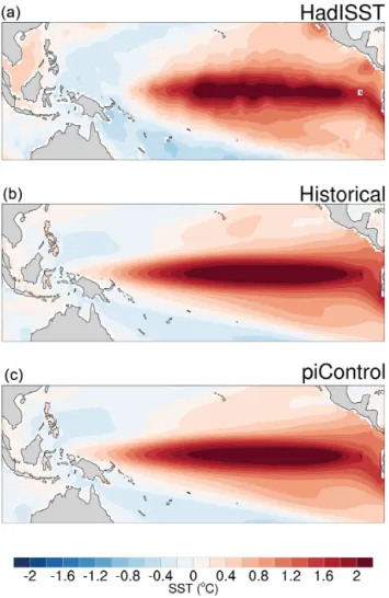
The ability of the CMIP5/PMIP3 and CMIP6/PMIP4 mod-els (hereafter, “CMIP” modmod-els) used in this study to simulate the present-day SST pattern is first evaluated in comparison with HadISST observations (Rayner et al., 2003) as shown in Fig. 1. Consistent with other studies of coupled GCMs (Bellenger et al., 2014; Collins et al., 2010), the models are generally biased toward overly cold SSTs in the central to western equatorial Pacific. Biases toward overly warm SSTs are present in the far eastern Pacific, again a common feature of GCMs generally resulting from a lack of sufficiently deep stratocumulus decks in eastern boundary regions (see review by Ceppi et al., 2017). The northern subtropics also appear to have similar biases, with colder-than-observed SSTs in the central Pacific and warm biases near the western coast of Mexico. The effect of comparison time period selection is apparent when the historical and piControl simulations are contrasted (Fig. 1c, d versus e, f); the piControl climate is roughly 1◦C colder on average than the historical simula-tion, leading to an apparent exacerbation of the cold-tongue bias and reduction in the warm bias in the eastern equatorial Pacific. The tropical Pacific SST biases in the newer CMIP6 models are smaller on average than those in the CMIP5 mod-els (see Fig. S1).
SST biases contribute to errors in the representation of pre-cipitation in the simulations. The Intertropical Convergence Zone (ITCZ) is generally shifted to the north (Fig. 2c, d), leading to a dry bias in the equatorial Pacific, which is
partic-Figure 1.Ability of the ensemble to simulate present-day sea surface temperature (SST) patterns: (a) DJF and (b) JJA SST climatology from HadISST observational dataset (Rayner et al., 2003) between 1971 and 2000, (c) DJF and (d) JJA model ensemble mean SST in historical simulations minus HadISST observations between 1971 and 2000, and (e) DJF and (f) JJA model ensemble mean SST in pre-industrial control simulations minus HadISST observations. Units are◦C. Stippling indicates that more than two-thirds of the ensemble members agree on the sign of the anomaly.
ularly pronounced during DJF (Fig. 2c). The equatorial cold SST bias also leads to the rising branch of the Walker cir-culation being shifted to the west, weakening atmospheric feedbacks (Bayr et al., 2018). South of the Equator, there is a wet bias in the location of the climatological South Pacific Convergence Zone (SPCZ) (Fig. 2c, d), consistent with previ-ously documented tendencies for CMIP-class models to pro-duce a so-called “double ITCZ” (Adam et al., 2018; Zhang et al., 2015). Once again, there are substantial differences between precipitation fields in the historical and piControl simulations (Fig. 2c, d versus e, f), with equatorial precipita-tion generally increased in historical. This is consistent with the expected intensification of the hydrological cycle under climate change (Held and Soden, 2006; Vecchi and Soden, 2007), for which some observational evidence exists during the 20th century (Durack et al., 2012). These differences are confounded somewhat by the slight differences in the com-position of the ensembles for piControl and historical sim-ulations (see Table 1). The CMIP6 models simulate smaller biases in tropical Pacific precipitation than CMIP5 models (see Fig. S2), consistent with the improved SST distribution. The spatial pattern of ENSO sea surface temperature anomalies is illustrated using the ensemble mean difference between composite El Niño and La Niña events, shown in Fig. 3. The magnitude of simulated historical and piCon-trol events (Fig. 3b, c) is quite close to the observed value
(Fig. 3a), with peak SST anomaly values of roughly 2.5◦C. However, the “centre of action” for ENSO is shifted west-ward relative to observations; this is a known feature of cou-pled GCMs and is related to the biases in mean SST (Bel-lenger et al., 2014). Because of this westward shift in the peak of El Niño and La Niña events, the magnitude of SST variability is overly weak in the far eastern Pacific (Fig. 3b, c). There may be substantial variation between the individ-ual model simulations, which is documented elsewhere (e.g. Bellenger et al., 2014). The ENSO SST anomalies in CMIP6 models are stronger than those in CMIP5 models in both the western and eastern equatorial Pacific (see Fig. S3).
We also evaluate the simulation of global temperature teleconnections with ENSO variability (Fig. 4). The ob-served warming over northern South America, Australia, and much of southeast Asia during DJF of the El Niño event peak (Fig. 4a) is reproduced by the CMIP ensemble mean (Fig. 4c), although the magnitudes of the temperature anoma-lies appear weaker than observed. The teleconnection to the Atlantic and Indian oceans likewise appears reliable, with comparable magnitudes of surface warming appearing in the models relative to observations. The models appear to have the most difficulty in representing teleconnections to the higher latitudes; the strong warming over northern North America during DJF (Fig. 4a) is significantly underestimated in the models (Fig. 4c, e), as is the cooling over
north-Figure 2.Ability of the ensemble to simulate present-day precipitation patterns: (a) DJF and (b) JJA SST climatology from the GPCP observational dataset (Adler et al., 2003) between 1979 and 1999, (c) DJF and (d) JJA model ensemble mean precipitation in historical simulations minus GPCP observations between 1979 and 1999, and (e) DJF and (f) JJA model ensemble mean precipitation in pre-industrial control simulations minus GPCP observations. Units are mm d−1. Stippling indicates that more than two-thirds of the ensemble members agree on the sign of the anomaly.
ern Eurasia. The same general tendencies hold during JJA (Fig. 4b, d, f); here, notable model–observation disagreement is apparent over the eastern half of North America, southern South America, and the southwestern Pacific. This latter fea-ture may relate to model difficulties with representing SPCZ dynamics (Brown et al., 2013).
Model performance in simulating ENSO temperature tele-connections is reflected in the structure of ENSO precipita-tion teleconnecprecipita-tion biases, shown in Fig. 5. In DJF, when El Niño events typically peak, drying occurs in the western Pacific warm pool and over the Amazon in the reanalysis (Fig. 5a); this drying persists in JJA but is reduced (Fig. 5b). In both cases, the models underestimate the magnitude of South American precipitation teleconnections; additionally, the western Pacific drying is shifted westward due to the bias in mean SST (Fig. 5c, d). Precipitation teleconnections to North America are overly weak in the simulations during both DJF and JJA, as are the tropical Atlantic anomalies.
In summary, the spatial pattern of ENSO SST variability and the remote teleconnections of temperature and precip-itation in response to ENSO are reasonably well simulated in the CMIP models and particularly in the ensemble mean. We therefore examine the changes in ENSO in these models under a range of past and future climate conditions.
4 Mean state changes
Changes in the mean state of the tropical Pacific are eval-uated for each experiment relative to the piControl simula-tion. This provides the context for consideration of changes in ENSO amplitude and teleconnections in the subsequent sections. Figures 6 and 7 summarise the seasonal response (DJF and JJA) of the model ensemble to different forcing during the three palaeoclimate experiments (midHolocene, lgm, and lig127k) and two idealised future warming sce-narios (1pctCO2 and abrupt4xCO2) for surface temperature (Fig. 6) and precipitation (Fig. 7).
For the last interglacial (lig127k), ensemble changes in surface temperatures (Fig. 6e, f) exhibit a strong seasonal-ity that is consistent with lig127k minus piControl insolation anomalies (see Otto-Bliesner et al., 2017). More specifically, in JJA, regions located at tropical and subtropical latitudes show warming (of about 0.5 to 2◦C). Indeed, during boreal
summer, positive insolation anomalies reach their maximum in the Northern Hemisphere (NH) and extend into the trop-ics and the Southern Hemisphere (SH). In contrast, in DJF, negative insolation anomalies are large in SH and NH equa-torward of 40◦N, and tropical and subtropical latitudes show cooling (mostly of about 1◦C). Similar patterns, although much weaker and spatially constrained, are shown for the midHolocenesimulation (Fig. 6a and b for DJF and JJA,
re-Figure 3.Evaluation of the ENSO SST anomaly pattern. Compos-ite El Niño minus La Niña sea surface temperature anomaly from (a) the HadISST observational dataset between 1871 and 2012, (b) model ensemble average from the historical simulations be-tween 1850 and 2005 (for CMIP5 models) or 1850 and 2015 (for CMIP6 models), and (c) model ensemble average from the pre-industrial control simulations. Units are◦C.
spectively), with small anomalies in both seasons. A small cooling of ∼ 0.5◦C is shown over the equatorial regions of the eastern (central) Pacific during DJF (JJA). No warming, however, is shown in the midHolocene simulation in either season. Based on the sign and magnitude of the insolation anomalies for both the midHolocene and (more so) lig127k simulations, the model ensemble mean state changes for both of these simulations are consistent with previous modelling and proxy reconstruction studies (see, e.g. Otto-Bliesner et al., 2013).1
The lgm ensemble mean shows cooling of around 2–3◦C in the tropical Pacific in both DJF and JJA (Fig. 6c, d),
consis-1Further analysis and description of the results of these PMIP4
experiments can be found in other articles in this special issue – e.g. Brierley et al. (2020) for midHolocene and Otto-Bliesner et al. (2020) for lig127k.
tent with previous modelling studies and proxy reconstruc-tions (Ballantyne et al., 2005; MARGO Project Members et al., 2009; Masson-Delmotte et al., 2014; Otto-Bliesner et al., 2009). For the idealised future scenarios, the tropical Pacific warms (by 1–3◦C in the 1pctCO2 case and more than 3◦C in the abrupt4xCO2 case), with largest warming in the equato-rial region. In the case of the abrupt4xCO2 simulations, the ensemble mean warming is largest in the eastern and cen-tral Pacific, particularly in DJF, whereas the 1pctCO2 ensem-ble shows enhanced warming extending across the equatorial Pacific. This enhanced equatorial warming is a recognised feature of anthropogenic climate warming (DiNezio et al., 2009; Liu et al., 2005; Xie et al., 2010) and has important implications for ENSO, leading to more frequent extreme El Niño events in a warmer climate (Cai et al., 2014; Wang et al., 2017).
Regarding ensemble precipitation anomalies, in the lig127ksimulations (Fig. 7e, f), the weaker Australian mon-soon (drier conditions over northern Australia in DJF) and the enhanced North American monsoon (wetter conditions over northern South America in JJA) are consistent with a northward shift of the mean seasonal position of the ITCZ (over the oceans) and the associated tropical rainfall belt (over the continents). As for surface temperatures, the mid-Holoceneensemble mean (Fig. 7a, b) shows similar spatial patterns of mean state precipitation change to the lig127k case but with smaller magnitude. The Australian monsoon (North American monsoon) is weaker (stronger) in the mid-Holoceneensemble mean relative to piControl, just less so than the lig127k simulation. Drying in the midHolocene sim-ulation is larger in the western Pacific than for lig127k. Mechanisms and drivers for precipitation changes over the tropics in last interglacial climates are still unclear and rep-resent an active area of research (see, e.g. Scussolini et al., 2019; Otto-Bliesner et al., 2020).
Precipitation changes in the lgm ensemble (Fig. 7c, d) show a drying over the Maritime Continent, Australia, and southeast Asia. Precipitation in the ITCZ over the tropical Pacific is also reduced, particularly in JJA, in response to cooler SSTs. Precipitation is increased in the western Pacific and on the northern edge of the SPCZ, indicating a north-ward displacement of the SPCZ, as found in previous stud-ies (Saint-Lu et al., 2015). In the 1pctCO2 and abrupt4xCO2 simulations (Fig. 7g–j), precipitation increases in the equato-rial Pacific where SST warming is greatest (e.g. Chadwick et al., 2013; Xie et al., 2010), with some drying on the northern edge of the ITCZ, particularly in the eastern Pacific. Drying also occurs in the southeast Pacific, where warming is rela-tively small and trade winds are intensified, leading to drying of the eastern edge of the SPCZ in DJF (Brown et al., 2013; Widlansky et al., 2013).
Previous studies have noted that changes in tropical pre-cipitation are strongly influenced by the spatial pattern of SST change (Chadwick et al., 2013; Xie et al., 2010). Such changes in SST gradients are also linked to changes in the
Figure 4.Evaluation of the ENSO temperature teleconnections. Composite El Niño minus La Niña surface temperature anomaly from (a) DJF and (b) JJA from the C20 reanalysis (Compo et al., 2011) between 1871 and 2010, (c) DJF and (d) JJA model ensemble mean from the historical simulations between 1850 and 2005 (for CMIP5 models) or 1850 and 2015 (for CMIP6 models), and (e) DJF and (f) JJA model ensemble mean from the pre-industrial control simulations. Units are◦C.
Walker circulation (Bayr and Dommenget 2013; Bayr et al., 2014). We therefore also plot the relative SST change, with the mean over the tropical domain (25◦N–25◦S, 100◦E–
80◦W) subtracted, in Fig. S4. Comparison of the precip-itation changes in Fig. 7 and the relative SST changes in Fig. S4 confirms that there is generally close agreement, with regions of relative warming experiencing increased precipi-tation and regions of relative cooling becoming drier in the ensemble mean.
5 ENSO amplitude changes
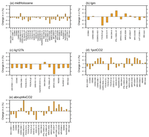
The amplitude of ENSO, as measured by the standard de-viation of SST from the NINO3.4 region, is shown for each model in each experiment in Fig. 8. The amplitudes of ENSO in the piControl simulation from each model are also shown for reference. The percentage change in ENSO amplitude in the experiments relative to piControl is shown in Fig. 9, and the ensemble mean change and minimum and maximum model changes are given in Table 2.
In the midHolocene simulations, a large majority (26 out of 30) of models show a decrease in ENSO variability, with the only exceptions being CMIP5 models (CSIRO-Mk3-6-0 and MRI-CGCM3) and CMIP6 models (INM-CM4-8 and
NorESM2-LM). Most of these changes are small, however, with few models showing more than a ∼ 20 % decrease (Figs. 8a and 9a). This is consistent with previous model studies, which generally show a smaller reduction in mid-Holocene ENSO amplitude than implied by proxy records (e.g. Emile-Geay et al., 2016), as discussed in Sect. 1. A similarly consistent reduction in ENSO amplitude is found for the lig127k simulations (Figs. 8c and 9c), with 10 out of 12 models showing a reduction in amplitude, typically of at least 20 %.
In contrast, a much less consistent response is found for the lgm, 1pctCO2, and abrupt4xCO2 simulations. In all of these simulations, the sign of change in amplitude of ENSO is approximately equally spread between increases and de-creases across the set of models. In the lgm simulations (Figs. 8b and 9b), some models (e.g. FGOALS-g2) show a large decrease in variability of over 40 % and others (e.g. IPSL-CM5A-LR) show large increases of up to ∼ 40 %. Likewise, in the 1pctCO2 simulations (Figs. 8d and 9d), ENSO variability is again highly model dependent, with the range including large decreases of over ∼ 20 % in some mod-els (e.g. CCSM4) to large increases of up to ∼ 40 % in others (e.g. MPI-ESM-P). The same is true for the abrupt4xCO2 simulations (Figs. 8e and 9e), with the range including large
Figure 5.Evaluation of the ENSO precipitation teleconnections. Composite El Niño minus La Niña precipitation anomaly from (a) DJF and (b) JJA from the C20 reanalysis (Compo et al., 2011) between 1871 and 2010, (c) DJF and (d) JJA model ensemble mean from the historical simulations between 1850 and 2005 (CMIP5)/2015 (CMIP6), and (e) DJF and (f) JJA model ensemble mean from the pre-industrial control simulations. Units are mm d−1.
Table 2.Multi-model mean change in ENSO amplitude (%) based on NINO3.4 standard deviation for each experiment relative to the pre-industrial control for all models, CMIP5/PMIP3 models, and CMIP6/PMIP4 models. Note that CMIP5/PMIP3 does not include lig127k experiment. Values in brackets for all models are the minimum and maximum model values.
All models’ CMIP5 CMIP5 CMIP6 CMIP6 ENSO ENSO number ENSO number Experiment change % change % models change % models midHolocene −8.4 (−36.8 to 18.5) −6.9 14 −9.7 16 lgm −4.8 (−46.9 to 32.5) −4.7 9 −4.8 3 lig127k −20.6 (−54.2 to 10.3) – – −20.6 12 1pctCO2 5.6 (−33.2 to 34.1) 1.4 13 11.6 9 abrupt4xCO2 2.2 (−46.3 to 57.7) 3.0 12 1.4 11
decreases of over ∼ 40 % in some models (e.g. GISS-E2-R) to large increases of up to ∼ 50 % in others (e.g. CSIRO-Mk3-6-0). This is consistent with previous studies showing little agreement on future projections of ENSO amplitude change (Collins et al., 2010, 2014).
Comparing the absolute magnitudes of ENSO amplitude in all simulations (Fig. 8), the standard deviation ranges (i.e. between the models showing the smallest and largest stan-dard deviations) are ∼ 0.7◦C in the midHolocene, ∼ 1.1◦C in the lgm, ∼ 0.2◦C in the lig127k, ∼ 0.7◦C in the 1pctCO2, and ∼ 1◦C in the abrupt4xCO2 simulations. The cold
cli-mate simulation and the extreme future run therefore show the largest spread between models, suggesting a lack of model agreement, whereas the midHolocene and lig127k simulations as well as the gradual future run have a much smaller spread between models.
Comparing the change in ENSO amplitude in all simula-tions (Fig. 9), we find that the midHolocene and lig127k sim-ulations have high inter-model agreement on the sign of the response, consistently showing lower ENSO variability rela-tive to the piControl simulation in both cases. The common factor between these simulations is the change in
seasonal-Figure 6.Ensemble mean seasonal changes in sea surface temperature in experiment minus pre-industrial control simulations: (a) DJF midHolocene, (b) JJA midHolocene, (c) DJF lgm, (d) JJA lgm, (e) DJF lig127k, (f) JJA lig127k, (g) DJF 1pctCO2, (h) JJA 1pctCO2, (i) DJF abrupt4xCO2, and (j) JJA abrupt4xCO2. The ensemble mean temperature pattern in the pre-industrial control simulations is shown as black contours. Units are◦C. Stippling indicates that more than two-thirds of the ensemble members agree on the sign of the change.
ity of insolation, which in both cases is increased in boreal summer, leading to a damped ENSO via a range of mecha-nisms discussed in Sect. 1 and also Sect. 7. In contrast, there is much less inter-model agreement in the cold climate sim-ulation (i.e. the lgm simsim-ulation) and the gradual and extreme future warming runs (i.e. the 1pctCO2 and abrupt4xCO2 simulations, respectively). While the model NINO3.4 time series have been detrended to remove long-term trends, the standard deviations shown in Figs. 8 and 9 may also in-clude contributions from variability at frequencies higher and lower than the ENSO range. These could be removed us-ing a band-pass filter with a 2- to 8-year window to isolate ENSO frequencies. Band-pass filtering reduces the ampli-tude of NINO3.4 variability in each simulation (not shown) but does not substantively alter the direction or magnitude
of changes in ENSO amplitude for any of the experiments (see Fig. S5).
Comparison of ENSO amplitude changes in CMIP5 and CMIP6 model ensembles shows generally strong agreement between the two generations of models (see Table 2 and Fig. S6). The ensemble mean reduction in midHolocene ENSO strength is somewhat greater for CMIP6 models than it is for CMIP5 models, while there is no lig127k experiment in CMIP5. Both sets of models simulate weaker ENSO am-plitude on average in the lgm experiments, although there are only three CMIP6 models available for this experiment. Both CMIP5 and CMIP6 models simulate an ensemble mean in-crease in ENSO amplitude in the idealised future 1pctCO2 and abrupt4xCO2 experiments, although with large inter-model spread (see Figs. 9 and S6).
Figure 7.Ensemble mean seasonal changes in precipitation in experiment minus pre-industrial control simulations: (a) DJF midHolocene, (b) JJA midHolocene, (c) DJF lgm, (d) JJA lgm, (e) DJF lig127k, (f) JJA lig127k, (g) DJF 1pctCO2, (h) JJA 1pctCO2, (i) DJF abrupt4xCO2, and (j) JJA abrupt4xCO2. The ensemble mean temperature pattern in the pre-industrial control simulations is shown as black contours. Units are mm d−1. Stippling indicates that more than two-thirds of the ensemble members agree on the sign of the change.
6 ENSO patterns and teleconnections
The anomalous pattern of El Niño minus La Niña SST com-posite for each experiment relative to piControl (see Fig. 3c) is shown in Fig. 10. The midHolocene and lig127k patterns (Fig. 10a, c) show negative SST anomalies in the central equatorial Pacific, indicating weakening of event amplitude, consistent with the average weakening of ENSO variability in these experiments (see Sect. 5 and Fig. 9). There is a much larger weakening of SST variability in the lig127k than the midHolocene case. The lgm SST pattern (Fig. 10b) shows negative anomalies in the central to western Pacific, indi-cating either an eastward shift of the ENSO pattern and/or weaker central Pacific variability. On the other hand, both the 1pctCO2 and abrupt4xCO2 composites (Fig. 10d, e) show positive Pacific SST anomalies associated with ENSO
at the Equator, with the largest values in the central Pa-cific, and high model agreement. This suggests an increased ENSO variability among the ensemble, particularly for the abrupt4xCO2simulations, despite the disagreement between model ENSO amplitude changes discussed in Sect. 5.
The global temperature and precipitation teleconnections with ENSO for each experiment relative to piControl are shown in Figs. 11 and 12. As discussed above, both lig127k and midHolocene simulations show weaker ENSO SST vari-ability relative to piControl (Fig. 10a, c). The lig127k sim-ulations have a much greater weakening of the ENSO SST and temperature patterns (Figs. 10c and 11e, f) than any of the other simulations (although based on a small number of models), with cooler SSTs in the central Pacific. The mid-Holocene ENSO SST and temperature pattern (Figs. 10a and 11a, b) is a weaker version of the lig127k response.
Figure 8.Amplitude of ENSO measured from standard deviation of NINO3.4 index (◦C) in piControl simulations (grey bars) and (a) mid-Holocene(dark green bars), (b) lgm (blue bars), (c) lig127k (light green bars), (d) 1pctCO2 (dark red bars), and (e) abrupt4xCO2 (light red bars) simulations. Model names are given below plots. Multi-model (MM) mean is also shown.
The ENSO precipitation teleconnection in the lig127k sim-ulations (Fig. 12e, f) consists of a weakening of the pi-Control ENSO precipitation pattern, with much drier con-ditions in the equatorial Pacific and over the SPCZ during El Niño events. The midHolocene ENSO precipitation pattern (Fig. 12a, b) is again a weaker version of the lig127k ENSO precipitation response.
The lgm simulations show cooler SSTs in the western trop-ical Pacific in the ENSO composite (Fig. 10b), consistent with a weakening of ENSO variability in this region. Cool anomalies over Australia and warm anomalies over North America are also evident (Fig. 11c, d). As expected, given the colder global mean temperatures (Fig. 6), precipitation associated with ENSO is reduced in the tropical Pacific and the overall hydrological cycle is weaker (Fig. 12c, d). Re-mote responses include wetter conditions over Australia and drier conditions over North America, somewhat resembling a La Niña pattern, although with low model agreement.
In contrast to the lgm experiments, the 1pctCO2 and abrupt4xCO2simulations are much warmer than the other experiments (Fig. 6). The largest temperature anomalies are seen for the abrupt4xCO2 simulations (Fig. 11i, j), which also had increased amplitude of SST variability in the cen-tral Pacific (Fig. 10e). The abrupt4xCO2 experiment shows warmer temperatures globally during El Niño events, par-ticularly over continents and high northern latitudes (ex-cept Greenland in DJF). It is possible that elements of the pattern in this experiment arise from the linear detrend-ing faildetrend-ing to sufficiently remove the transient changes in mean state (Sect. 2.3). The 1pctCO2 simulations (Fig. 11g, h) show a similar but much weaker response. The pre-cipitation response to ENSO (Fig. 12) is enhanced in the abrupt4xCO2 and 1pctCO2 simulations relative to piCon-trol, with increases in precipitation in the equatorial Pacific and decreases in the subtropics, as ENSO influences tropical atmospheric circulation and therefore the hydrological cycle
Figure 9. Change in amplitude of ENSO measured from standard deviation of NINO3.4 index relative to piControl amplitude (%) in (a) midHolocene, (b) lgm, (c) lig127k, (d) 1pctCO2, and (e) abrupt4xCO2. Model names are given below plots. MM mean is also shown.
(Lu et al., 2008; Nguyen et al., 2013). This is consistent with previous studies showing intensified ENSO temperature and precipitation impacts in a warmer climate (e.g. Power et al., 2013; Power and Delage, 2018).
The relationship between changes in ENSO and changes in the annual cycle, zonal and meridional SST gradient are investigated for all models and experiments (Fig. 13). The change in ENSO amplitude based on the standard devia-tion of NINO3.4 (relative to piControl) is plotted against the change in annual cycle of NINO3.4 SST in Fig. 13a, with a weak positive correlation between the two variables. The change in ENSO amplitude was found to have no significant correlation with the change in equatorial Pacific zonal SST gradient (defined as 5◦S–5◦N, 150◦E–170◦W minus 5◦S– 5◦N, 120–90◦W), shown in Fig. 13b. Finally, the relation-ship between eastern Pacific rainfall and meridional SST gra-dient (Cai et al., 2014) is investigated (Fig. 13c). The merid-ional SST gradient in the eastern Pacific is defined as the average SST over the off-equatorial region (5–10◦N, 150–
90◦W) minus the average over the equatorial region (2.5◦S– 2.5◦N, 150–90◦W). The strength of eastern Pacific El Niño rainfall is represented as the changes in ENSO composite precipitation over the NINO3 region (5◦S–5◦N, 150–90◦W) normalised by the NINO3.4 standard deviation used to iden-tify the composited events. This normalisation aims to re-move the impact of the changes in ENSO variability doc-umented between the experiments (e.g. Power and Delage, 2018). The significant negative correlation is consistent with the analysis demonstrated by Cai et al. (2014) and Collins et al. (2019), but this analysis approach allows the relationship to be visualised across many more simulations and experi-ments. This relationship appears to be fundamental feature of ENSO behaviour rather than just a response to greenhouse gas forcing.
Figure 10.The changes in the SST pattern associated with ENSO in each experiment compared with piControl. The ensemble mean difference between the SST composites of each model’s El Niño minus La Niña (defined as ±1 standard deviation) in the (a) mid-Holocene, (b) lgm, (c) lig127k, (d) 1pctCO2, and (e) abrupt4xCO2 experiments minus the same pattern for the piControl simulations is shown. The ensemble mean ENSO SST patterns in the piControl simulations are shown as black contours. Stippling indicates that more than two-thirds of the ensemble members agree on the sign of the change.
7 Mechanisms and discussion
There is evidence that the mid-Holocene, a period of sup-pressed ENSO variability, featured a stronger zonal gradi-ent in the tropical Pacific mean SST than the 20th cgradi-entury, namely “La Niña-like conditions” (Barr et al., 2019; Gagan and Thompson, 2004; Koutavas et al., 2002; Luan et al., 2012; Shin et al., 2006). In contrast, proxy records suggest that the mean state of the tropical Pacific during the Pliocene warm period featured sustained El Niño-like conditions (Fe-dorov et al., 2006; Wara et al., 2005). It is likely that the weak zonal SST gradient in the Pliocene was less favourable for ENSO occurrence (Brierley, 2013; Manucharyan and Fe-dorov, 2014). These contradictory responses imply that the dynamical mechanisms determining the relationship between the zonal gradient in mean SST and ENSO amplitude (e.g. Sadekov et al., 2013) must consist of several processes. The relationship between ENSO amplitude and SST gradient may also be nonlinear (Hu et al., 2013). This lack of consistent or linear relationship between zonal SST gradient and ENSO amplitude is supported by the results presented here, shown in Fig. 13b.
During the mid-Holocene, the reduced tropical insolation led to the cooling of the tropical Pacific, directly producing a La Niña-like condition. Under La Niña-like conditions, the air–sea coupling strength is reduced due to a suppressed con-vective instability, and thus ENSO variability is suppressed (Liu et al., 2000; Roberts et al., 2014). The stronger sea-sonality in insolation over the Northern Hemisphere asso-ciated with the precession cycle resulted in a stronger an-nual cycle, which could also act to reduce ENSO variability through the intensified annual-frequency entrainment (Liu, 2002; Pan et al., 2005). A similar but stronger precession ef-fect due to the higher eccentricity during the last interglacial period was also found to have a relatively weak ENSO ampli-tude in palaeoproxy records (Hughen et al., 1999; Tudhope et al., 2001) and climate model simulations (An et al., 2017; Salau et al., 2012). However, the mid-Holocene simulations of PMIP2/3 mostly showed a reduction of both annual cycle and ENSO amplitude (An and Choi, 2014; Masson-Delmotte et al., 2014).
The reduced annual cycle over the tropical eastern Pa-cific is attributed to the relaxation of eastern PaPa-cific upper-ocean stratification due to the annual downwelling Kelvin wave forced by western Pacific wind anomalies (Karamperi-dou et al., 2015) or the deepening of ocean mixed layer depth associated with the northward shift of the ITCZ (An and Choi, 2014). Therefore, the mid-Holocene ENSO variabil-ity in PMIP2/3 may be deemed to the result of the coun-terbalance between the reduction due to the weaker air–sea coupling and the intensification due to the reduced frequency entrainment (An and Choi, 2014). Other factors may include coupling of the circulation in the eastern Pacific with the North American monsoon (implying dynamical damping of upwelling in the eastern Pacific) and an increased southeast
Figure 11.The changes in the seasonal temperature teleconnection pattern associated with ENSO in each experiment compared with the pre-industrial control. The ensemble mean difference between the surface temperature composites of each model’s El Niño minus La Niña (defined as ±1 standard deviation) in the (a, b) midHolocene, (c, d) lgm, (e, f) lig127k, (g, h) 1pctCO2, and (i, j) abrupt4xCO2 experiments minus the same pattern for the piControl simulations is shown. The ensemble mean ENSO patterns in the piControl simulations are shown as black contours. Stippling indicates that more than two-thirds of the ensemble members agree on the sign of the change.
Asian monsoon which strengthens winds in the western Pa-cific. Alternatively, An et al. (2010) and An and Choi (2013) argue that the change in annual cycle amplitude is not a cause of change in ENSO amplitude; it is the changes in the mean climate state that modify both the ENSO and annual cycle amplitudes in the opposite way. The analysis presented here would appear to support the argument that there is no con-sistent relationship between changes in the amplitude of the annual cycle and changes in the ENSO variability (Fig. 13a).
ENSO variability can be suppressed or enhanced by re-mote forcing. For example, the enhanced Asian summer monsoon also leads to La Niña-like conditions via increasing strength of the tropical Pacific trade winds and the resultant enhanced equatorial upwelling (Liu et al., 2000). Sensitivity experiments with fully coupled climate models demonstrate that greening of the Sahara during the mid-Holocene could reduce ENSO variability through affecting the Atlantic Niño (Zebiak, 1993) and Walker circulation, finally decreasing up-welling and deepening of the thermocline in the eastern
Pa-Figure 12.The changes in the seasonal precipitation teleconnection pattern associated with ENSO in each experiment compared with the pre-industrial control. The ensemble mean difference between the precipitation composites of each model’s El Niño minus La Niña (defined as ±1 standard deviation) in the (a, b) midHolocene, (c, d) lgm, (e, f) lig127k, (g, h) 1pctCO2, and (i, j) abrupt4xCO2 experiments minus the same pattern for the piControl simulations is shown. The ensemble mean ENSO patterns in the piControl simulations are shown as black contours. Stippling indicates that more than two-thirds of the ensemble members agree on the sign of the change.
cific (Pausata et al., 2017). The freshwater perturbation ex-periments, so-called “water hosing experiment” that lead to a weakening of the Atlantic Ocean meridional overturning circulation, showed a reduced seasonal cycle and enhanced ENSO variability through the inter-basin atmospheric tele-connection (Braconnot et al., 2012; Masson-Delmotte et al., 2014; Timmermann et al., 2007).
More sophisticated feedback analysis revealed that the re-duction of ENSO variability is due to either the increase of the negative feedback by the mean current thermal
advec-tion (An and Bong, 2018) or the reducadvec-tion of the major pos-itive feedback processes (thermocline, zonal advection and Ekman feedbacks) (Chen et al., 2019a; Tian et al., 2017). The negative feedback due to the thermal advection by the mean current was intensified by the stronger cross-equatorial winds associated with the northward migration of the ITCZ (e.g. An and Choi, 2014), and the positive dynamical feed-back was suppressed due to the strengthening of the mean Pa-cific subtropical cell (Chen et al., 2019a). Therefore, the lin-ear stability of ENSO during the mid-Holocene was reduced
Figure 13.Relationships across all experiments and all models: (a) ENSO amplitude change (%) versus change in the annual cycle (%), (b) ENSO amplitude change (◦C) versus zonal SST gradient change (◦C), and (c) NINO3 precipitation for ENSO composite versus merid-ional SST gradient change (◦C). All changes are relative to piControl; see text for details. Experiments are identified as follows: blue squares indicate lgm, dark green circles indicate midHolocene, light green diamonds indicate lig127k, dark red stars indicate 1pctCO2, and light red triangles indicate abrupt4xCO2 (after bar charts in Fig. 8). Correlation coefficients are shown for each plot.
through the dedicated balance among the various feedback processes, but the change in each feedback process is model dependent. External processes were also proposed as a sup-pression mechanism for mid-Holocene ENSO. For example, the Pacific meridional mode became weaker during the mid-Holocene; thereby, ENSO has a relatively lower chance of being triggered (Chiang et al., 2009); the weaker ocean strat-ification due to the warm water subduction from the subtrop-ical ocean decreases ENSO stability (Liu et al., 2000).
How ENSO activity will change in response to anthro-pogenic global warming still remains uncertain (Cai et al., 2015a; Christensen et al., 2014; Collins et al., 2010). Ob-servations show that ENSO variability has increased under greenhouse warming in the recent past (Zhang et al., 2008), which is also shown in CMIP5 climate model simulations (Cai et al., 2018). During the transient period of global warm-ing, the tropical SSTs warm much faster than the subsurface ocean and leads to a shallower and stronger thermocline in the equatorial Pacific (An et al., 2008), which enhances the
ocean–atmosphere coupling and amplifies the ENSO vari-ability (Zhang et al., 2008). A gradually intensified ENSO from the mid-Holocene to late Holocene also appears in a long-transient simulation since the last 21 000 years (Liu et al., 2014) and of the last 6000 years (Braconnot et al., 2019). For the equilibrium response to global warming, the subsur-face ocean will eventually warm up and reduce the vertical temperature gradient and weaken the ENSO variability. For instance, during the Pliocene warm period, the most recent period in the past with carbon dioxide concentrations similar or higher than today, SST reconstructions from the tropical Pacific show a reduced zonal SST gradient during this pe-riod, implying sustained El Niño-like conditions (Dekens et al., 2007; Fedorov et al., 2006; Wara et al., 2005) as well as a deeper thermocline with weaker thermocline feedback (White and Ravelo, 2020).
It is still a topic of debate as to whether the tropical climate mean state response to current global warming will be El Niño-like or La Niña-like (Cane et al., 1997; Collins, 2005;
Merryfield 2006; An et al., 2012; Collins et al., 2010; Lian et al., 2018). Moreover, the global warming-induced tropi-cal Pacific SST pattern seems to be less effective in chang-ing ENSO activity (An and Choi, 2015). The strong inter-nal modulation of ENSO activity over decadal-to-centennial timescales also obscures the actual global warming impact on ENSO variability (e.g. Wittenberg, 2009). So far, the future ENSO activity reflected in SST anomalies obtained from CMIP5 models is not distinguishable from the histori-cal ENSO activity (Christensen et al., 2014).
The enhancement and increasingly frequent occurrence of ENSO-driven extreme atmospheric responses to future global warming are strongly supported by model studies. This includes extreme rainfall events and extreme equator-ward swings of the SPCZ (Cai et al., 2014, 2015a, 2012) and extreme weather events through teleconnections (Cai et al., 2015a; Yeh et al., 2018). The changes in these extremes are due to the nonlinearity of atmospheric response to ENSO SSTs, especially with a warmer ocean surface. The chang-ing amplitude of the extremes with changchang-ing meridional SST gradient is a feature of past climates as well as future cli-mates. This is demonstrated in Fig. 13c, which shows an in-crease in the ENSO composited precipitation with inin-creased SST gradient. However, most current GCMs still inaccu-rately simulate many aspects of the historical ENSO such as the far westward extent of the Pacific cold tongue (Taschetto et al., 2014), ENSO-related precipitation anomalies (Dai and Arkin, 2017), ENSO feedbacks (Bayr et al., 2019; Bellenger et al., 2014; Kim et al., 2014; Kim and Jin, 2011; Lloyd et al., 2012), and ENSO asymmetry in amplitude, duration, and transition (e.g. Chen et al., 2017; Zhang and Sun, 2014). Therefore, the accuracy of the future projections of ENSO will be guaranteed only when most coupled GCMs can simu-late the observed modern-day ENSO more skilfully than they can at present.
8 Summary and conclusions
We have presented a summary of ENSO amplitude and tele-connections changes in the most recent previous generation (CMIP5) and the new generation (CMIP6) of coupled cli-mate models for past and future clicli-mates. The analysed simu-lations include the Last Glacial Maximum climate (lgm), past interglacial climates (lig127k and midHolocene), and future idealised projections (abrupt4xCO2 and 1pctCO2), using the pre-industrial climate (piControl) as the reference state.
We first evaluated a 30-year climatology from the histor-ical simulation against HadISST observation from 1971 to 2000. Similarly to the previous generations of climate mod-els, the CMIP5 and CMIP6 models have cold biases in SST in the central to western equatorial Pacific, as well as in the subtropical Pacific. Warm SST biases are present in the east-ern equatorial Pacific. The piControl climate is about 1◦C colder on average than the historical climate, leading to an
apparent exacerbation of the cold-tongue bias and reduction in the warm bias in the eastern equatorial Pacific. These bi-ases in SST lead to a strong and northward shift of ITCZ, a dry bias along the equatorial Pacific, and appearance of a “double ITCZ” as in previous CMIP-class simulations. SST and precipitation biases are generally slightly smaller in the new generation of CMIP6 models than in the CMIP5 models. The simulated ENSO pattern well resembles the observations with a slight displacement to the west; similarly, the ENSO temperature and precipitation teleconnections are well simu-lated compared with observations.
The mean state changes were examined relative to the pi-Controlsimulation. In the lig127k simulations, strong sea-sonal insolation anomalies lead to tropical and subtropical SST cooling of 0.5–2◦C in DJF and JJA. No large-scale warming is found in the midHolocene simulations, but a slight cooling of 0.5◦C occurs in the eastern Pacific in DJF
and in the central Pacific in JJA. In the lgm simulations, 2–3◦C cooling is found in the tropical Pacific. For the fu-ture scenarios, the tropical Pacific warms by 1–3◦C in the 1pctCO2case and more than 3◦C in the abrupt4xCO2 case. During the lig127k and midHolocene simulations, the ITCZ shifts northward, leading to a weakened Australian summer monsoon and enhanced North American summer monsoon. In the lgm simulations, the ITCZ is intensified over the trop-ical Pacific, with drier conditions over the Maritime Conti-nent, Australia, and southeast Asia, while wetter conditions are found in the western Pacific and on the northern edge of the SPCZ. In the 1pctCO2 and abrupt4xCO2 simulations, precipitation increases in the equatorial Pacific following the largest SST warming, with some drying on the northern edge of the ITCZ and in southeast Pacific in DJF.
The majority of models show a decrease in ENSO variabil-ity in the lig127k and midHolocene simulations. The reduc-tion of ENSO variability in lig127k ranges to more than 40 %, while only one model shows more than a ∼ 20 % decrease in ENSO variability in midHolocene. This is consistent with previous model studies of mid-Holocene ENSO, which gen-erally show a smaller reduction in amplitude than implied by proxy records.
The changes in ENSO variability in lgm, 1pctCO2 and abrupt4xCO2simulations are highly model dependent, with the sign of change approximately equally divided between increases and decreases of up to 40 % to 50 % across the set of models. This is also consistent with previous studies show-ing little agreement on ENSO amplitude change under LGM conditions (Masson-Delmotte et al., 2014) or in future pro-jections (Collins et al., 2014).
The ensemble mean weakening of ENSO in the lgm simu-lations is characterised by a cooling in the central and west-ern Pacific. Cooling over Australia and warming over North America are also evident. The changes in the ENSO tem-perature teleconnections show cooling in the central Pacific in lig127k and midHolocene, and significant global warming in the abrupt4xCO2 simulation, with strong warming


![[PDF] Tutoriel Arduino labview enjeux et pratique | Cours Arduino](data:image/gif;base64,R0lGODlhAQABAIAAAP///wAAACH5BAEAAAAALAAAAAABAAEAAAICRAEAOw==)