HAL Id: hal-01184563
https://hal.archives-ouvertes.fr/hal-01184563
Submitted on 16 Aug 2015
HAL is a multi-disciplinary open access
archive for the deposit and dissemination of
sci-entific research documents, whether they are
pub-lished or not. The documents may come from
teaching and research institutions in France or
abroad, or from public or private research centers.
L’archive ouverte pluridisciplinaire HAL, est
destinée au dépôt et à la diffusion de documents
scientifiques de niveau recherche, publiés ou non,
émanant des établissements d’enseignement et de
recherche français ou étrangers, des laboratoires
publics ou privés.
Copyright
Simon Eickhoff, Bertrand Thirion, Gaël Varoquaux, Danilo Bzdok
To cite this version:
Simon Eickhoff, Bertrand Thirion, Gaël Varoquaux, Danilo Bzdok. Connectivity-Based Parcellation:
Critique and Implications. Human Brain Mapping, Wiley, 2016, pp.22. �10.1002/hbm.22933�.
�hal-01184563�
For Peer Review
Connectivity-based parcellation:
critique & implications
Simon B. Eickhoff1,2,*, Bertrand Thirion3, Gaël Varoquaux3, Danilo Bzdok1,2, 3,+,* Simon B. Eickhoff (s.eickhoff@fz-juelich.de)
Danilo Bzdok (danilo.bzdok@fz-juelich.de) 1
Institut für Neurowissenschaften und Medizin (INM-1), Forschungszentrum Jülich GmbH,
52425 Jülich, Germany &
2
Institut für klinische Neurowissenschaften und Medizinische Psychologie Heinrich-Heine Universität Düsseldorf
40225 Düsseldorf, Germany
Bertrand Thirion (bertrand.thirion@inria.fr) Gaël Varoquaux (gael.varoquaux@inria.fr) Danilo Bzdok (danilo.bzdok@inria.fr) 3
Parietal team, INRIA Neurospin, bat 145 CEA Saclay
91191 Gif-sur-Yvette, France
+
Corresponding author: Danilo Bzdok (danilo.bzdok@inria.fr)
*Authorship determined by coin flip
Abstract
Regional specialization and functional integration are often viewed as two fundamental principles of human brain organization. They are closely intertwined because each functionally specialized brain region is probably characterized by a distinct set of long-range connections. This notion has prompted the quickly developing family of connectivity-based parcellation (CBP) methods in neuroimaging research. CBP assumes that there is a latent structure of parcels in a region of interest (ROI). First, connectivity strengths are computed to other parts of the brain for each voxel/vertex within the ROI. These features are then used to identify functionally distinct groups of ROI voxels/vertices. CBP enjoys increasing popularity for the in-vivo mapping of regional specialization in the human brain. Due to the requirements of different applications and datasets, CBP has diverged into a heterogeneous family of methods. This broad overview critically discusses the current state as well as the commonalities and idiosyncrasies of the main CBP methods. We target frequent concerns faced by novices and veterans to provide a reference for the investigation and review of CBP studies.
Keywords
Brain parcellation, clustering, resting-state correlations, diffusion MRI, data-driven, statistical learning, statistical inference, double dipping
2 3 4 5 6 7 8 9 10 11 12 13 14 15 16 17 18 19 20 21 22 23 24 25 26 27 28 29 30 31 32 33 34 35 36 37 38 39 40 41 42 43 44 45 46 47 48 49 50 51 52 53 54 55 56 57 58 59 60
For Peer Review
Introduction
The human brain is commonly assumed to be organized in distinct modules (Brodmann, 1909; Vogt and Vogt, 1919). These could be described according to structure, connectivity, and function. Cortical areas can be conceptualized as patches of the brain that differ from their neighbors in terms of their microarchitecture (e.g., cyto-, myelo- and receptorarchitecture), connectivity (i.e., set of input and output connections), and function (e.g., lesion-induced behavior or electrophysiological responses) (Felleman et al., 1991; Van Essen, 1985). The conjunction of i) input and output connectivity of a cortical area and ii) its local infrastructure is thought to crucially determine what classes of computational problems (i.e., function) it can solve (Scannel et al., 1995; Mesulam 1998; Passingham et al., 2002; Saygin et al., 2012).
The correspondence between a cortical area and its axonal connectivity fingerprint has prompted connectivity-based parcellation (CBP) approaches (Behrens and Johansen-Berg, 2005; Wiegell et al., 2003). Capitalizing on the distinct connections of each area (Passingham et al., 2002), CBP divides a region of interest (ROI, i.e., a volume- or surface-based topographical definition) into distinct subregions. The key idea is to first compute a connectivity profile for each individual voxel or vertex in the ROI. The voxel/vertex-wise connectivity profiles are then used to group the ROI voxels/vertices such that connectivity is similar for the voxels/vertex within a group and different between groups. That is, distinct clusters are identified in the ROI by differences between long-rang interaction patterns of the voxels/vertices in the ROI. Historically, CBP has first been performed based on whole-brain structural (fiber) connectivity profiles as derived from diffusion magnetic resonance imaging (dMRI) (Behrens et al., 2003; Wiegell et al., 2003). Later, analogous approaches based on resting-state functional connectivity (RSFC) (Kim et al., 2010) and, most recently, meta-analytic connectivity modeling (MACM) (Eickhoff et al., 2011) have been introduced. On the one hand, previous investigations have demonstrated that CBP can reveal clusters that recover known histological parcellations (e.g., Bzdok et al., 2012; Johansen-Berg et al., 2005). On the other hand, there are also reports showing that CBP may yield more fine-grained subdivisions than classical cytoarchitectonic mapping (e.g., Clos et al., 2013). Hence, CBP-derived modules may be viewed as 'functional areas', although these are outlined by connectivity differences rather than function.
The ability of CBP methods to map functional areas led to rapid adoption by neuroimaging investigators (cf. Smith et al., 2013a). Yet, several circumstances encourage heterogeneity in this nascent field. Methodologically, the CBP procedure is based on practical choices inconsistent across laboratories. Importantly, no single package permitting CBP is, to the best of our knowledge, openly distributed at the moment. Rather, it seems that different research groups perform CBP analyses based on their own script library, in-house databases, and laboratory setups. However, sharing of code implementations and international collaboration on its successive improvement will hopefully contribute towards a widely accepted software infrastructure (cf. Pradal et al., 2013).
Challenges that typically arise in CBP studies will be discussed in different sections. We will start out with the purpose of CBP and the neurobiological conclusions that can be drawn from it. The subsequent sections deal with the initial, interrelated decision on the ROI definition and the connectivity aspect to be investigated. We will then outline the main clustering approaches and corresponding cluster-selection criteria. The ensuing CBP results frequently raise questions around statistical inference and double dipping, discussed in later parts of the manuscript. We finally reflect possible ways to capitalize on CBP results as a starting point for multi-modal
2 3 4 5 6 7 8 9 10 11 12 13 14 15 16 17 18 19 20 21 22 23 24 25 26 27 28 29 30 31 32 33 34 35 36 37 38 39 40 41 42 43 44 45 46 47 48 49 50 51 52 53 54 55 56 57 58 59 60
For Peer Review
studies. All these issues are discussed below by providing overview, potential pitfalls, and possible solutions aimed at neuroimaging novices and experts. We hope that these considerations may ultimately help unify the dynamically developing spectrum of CBP methods.
2 3 4 5 6 7 8 9 10 11 12 13 14 15 16 17 18 19 20 21 22 23 24 25 26 27 28 29 30 31 32 33 34 35 36 37 38 39 40 41 42 43 44 45 46 47 48 49 50 51 52 53 54 55 56 57 58 59 60
For Peer Review
I Motivation
1.1 Aim
The principle of brain segregation guided by long-distance connections can be attractive from different perspectives, including the investigation of local functional differentiation, the creation of data-driven brain atlases, and catalyzing the inception of unprecedented hypotheses.
Location mapping. Comparing to other current neuroimaging approaches, CBP has the key strength to actually
map distinct brain areas. This can be opposed to either localizing a particular (dys)function or characterizing a
particular region. Most whole-brain association studies, be it functional MRI, voxel-based morphometry, lesion mapping, or most resting-state connectivity analyses, primarily elucidate the location in the brain of a particular effect such as the recruitment by a particular task, a differential response between two conditions, a difference between two groups, or the association with a particular phenotype. They are mapping cognitive, behavioral, and clinical aspects onto the brain. They do however not allow constructing a map from the brain itself (cf. Amunts et al., 2014 for a more detailed discussion). Put different, most neuroscientific methods associating behavior with aspects of neurobiology are naïve to underlying neurobiological compartments. While observing mappings between behavior and the brain, these methods are not well suited to establish or question the architecture of the brain itself (Frackowiak and Markram, 2015). That is, rather than providing a map of the brain, they provide a map of a particular functional or structural feature (such as recruitment by a particular task or aberrations in a particular group of patients) in brain space. The potency of brain-behavior interpretations can however be increased when constrained by knowledge of brain organization units (Devlin and Poldrack, 2007). CBP can propose such organizational units.
Altas mapping. CBP methods are capable of automatically compartmentalizing the human brain into
topographically delineated, functionally distinct regions (Behrens and Johansen-Berg, 2005). That is, 3D brain atlases can be obtained as quantitative models of brain segregation. In that context, an atlas represents a map of (parts of) the brain that assigns each location (voxel/vertex) to a particular structure and hence provides a segregation of the assessed volume into distinct modules. In whole-brain CBP, the ROI to be segregated covers the entire gray matter. By evaluating connectivity strengths from each gray-matter voxel/vertex to every other gray-matter voxel/vertex, a compartmental model of functional organization in the cerebral cortex can be derived. In local CBP, the ROI to be segregated covers a circumscribed part of gray matter. It can thus be evaluated whether that brain patch contains functionally distinct modules. As another important CBP variant, a-priori hypotheses can be introduced by measuring connectivity only to preselected brain regions, instead of the whole brain (e.g., Behrens et al., 2013; Bach et al., 2011; Sallet et al., 2013). In sum, CBP can readily propose 3D models of brain organization for use as reference atlases.
Hypothesis generation. Many currently employed neuroimaging methods test spatial hypotheses by either
localizing effects or characterizing a region, instead of providing explicit hints that encourage novel research hypotheses (cf. Biswal et al., 2010). CBP may be seen as an approach towards the generation of novel hypotheses on regional differentiation. These can subsequently be tested in hypothesis-driven experimental studies. For instance, exploratory CBP evidence supported existence of distinct subregions in the right temporo-parietal junction (Mars et al, 2012). This was subsequently confirmed by targeted neuroimaging studies based on cognitive fMRI experiments (Silani et al., 2013), ICA-based experiments (Igelstrom et al., 2015),
hypothesis-2 3 4 5 6 7 8 9 10 11 12 13 14 15 16 17 18 19 20 21 22 23 24 25 26 27 28 29 30 31 32 33 34 35 36 37 38 39 40 41 42 43 44 45 46 47 48 49 50 51 52 53 54 55 56 57 58 59 60
For Peer Review
driven meta-analysis (Krall et al., 2015), quantitative reviews (Schurz et al., 2014), as well as multivariate pattern analysis in clinical populations (Koster-Hale et al., 2013).
1.2 Neurobiological meaning
What does it actually mean to divide the brain based on differences in connectivity profiles? CBP performs a systematic summary of the Cortex cerebri by combining same tissue and separating different tissue according to an organizational criterion, namely, brain connectivity. Analogous to cytoarchitectonic mapping by microanatomical criteria (cf. Brodmann, 1909, pages 5 and 288-290), functional mapping by connectional criteria critically depends on the certainty that we have about the divisive criterion.
Cortical areas. From an anatomical perspective of brain segregation (Amunts et al., 2013), cortical areas are
believed to be distinguishable from their neighbors by featuring a distinct (micro)structure, distinct connectivity, and distinct function. In fact, function may follow naturally given that structure and connectivity are thought to conjointly enable locally specific neuronal computations (Passingham et al., 2002). As CBP is based on connectivity (true in a strict sense only for dMRI-CBP, cf. below), the defined clusters are not directly interpretable as cortical areas. Note that the current concepts of what constitutes a cortical area are mainly derived from studies of early sensory (Van Essen et al., 1992) and motor (Rizzolatti et al., 1988) brain systems. They may not be readily applicable to higher-level associative brain areas (Yeo et al., 2011), such as the dorsomedial prefrontal cortex (cf. Eickhoff et al., in press). Indeed, with increasing distance from sensory input processing, it is more and more difficult to relate the connectivity pattern of an area to its functional roles (Bzdok et al., 2013a; Bzdok et al., in press; Mesulam 1998; Yeo et al., 2011). Claims about cortical areas based on CBP results may therefore become more and more delicate with increasing level in the cerebral processing hierarchy.
One single versus multiple parallel subdivisions. From a more methodological perspective of brain
segregation, CBP does not address the neurobiological question whether there is a 'true' parcellation. It is employed to identify the 'optimal' clustering solution, in the sense of best describing the data. It is about the question whether different parcellation results for the same ROI capture different resolutions or dimensions of an underlying neurobiological organization (cf. Kelly et al., 2012; Amunts et al., 2014; Eickhoff and Grefkes 2011). The answer depends on the region of interest. For instance, previous CBP work on the insula (Kelly et al., 2012; Nanetti et al., 2009) and the right temporo-parietal junction (Bzdok et al., 2013b; Mars et al, 2012) have indicated close agreement between the parcellations based on different connectivity modalities. In contrast, parcellations of the posteromedial cortex diverged more strongly between dMRI- and RSFC-CBP studies (Cauda et al., 2010; Zhang and Li, 2012; Zhang et al., 2014). These observations corroborate the relevance of the conceptual differences between aspects of connectivity, such as dMRI, RSFC, and structural covariance. Moreover, there is probably no such thing as 'the connectivity' for a particular location. There may neither be 'the CBP parcellation.' Rather, brain segregation across connectivity modalities can possibly feature both similarity and dissimilarity.
Multi-modal comparison. Unfortunately, there are yet very few studies that address this fundamental question
of brain organization. Such a comparison across connectivity modalities is currently impeded by two key factors. On the one hand, results from previous CBP studies are rather inconsistently available to the community as
2 3 4 5 6 7 8 9 10 11 12 13 14 15 16 17 18 19 20 21 22 23 24 25 26 27 28 29 30 31 32 33 34 35 36 37 38 39 40 41 42 43 44 45 46 47 48 49 50 51 52 53 54 55 56 57 58 59 60
For Peer Review
image files, which renders most attempts to compare findings purely qualitative (Gorgolewski et al., in press). On the other hand, there appears to be a sentiment that a new CBP study in an already analyzed brain region is primarily a replication and hence lacking novelty. This discourages additional work on previously parcellated brain regions.
Meaning of CBP clusters. Given the biological and methodological characteristics of the most frequently used
anatomical and functional connectivity measures, we would suggest the following tentative distinction. For dMRI-CBP, the delineated clusters most likely reflect truly connectivity-defined modules, even in light of known artifacts (cf. below). In contrast, MACM-CBP reveals clusters that are probably functionally distinct modules even though the spectrum of brain functions is likely to be larger than what can be probed by neuroimaging techniques (cf. Mennes et al., 2013; Smith et al., 2009). That is, task-based functional connectivity might be limited by real-world behavior being richer than in-scanner behavior. The neurobiological nature of RSFC-CBP derived clusters might remain most uncertain. This is because the relation of resting-state correlations to anatomical connectivity, function, and the brain's housekeeping physiology is currently only incompletely understood (Biswal et al., 1995; Zhang and Raichle, 2010).
The insula. To take a concrete example, previous CBP results match some neurobiological dimensions of the
insula, but certainly not all of them (Fig. 1). On a microanatomical scale, investigations classically divided the insula into a rostroventral (agranular), rostrodorsal (dysgranular), and caudal (granular) portions in macaque monkeys (Mesulam and Mufson, 1982a). On a macroanatomical scale, the more rostral insula is preferentially connected to frontal regions, whereas the more caudal insula is preferentially connected to primary and secondary sensory as well as motor regions (Mesulam and Mufson, 1982b; Mufson and Mesulam, 1982a). On a developmental scale, anterior-posterior segregation in the human insula becomes observable within the first two years of life, as indicated by RSFC-CBP in infants (Alcauter et al., 2013). From the perspective of sensory input channels, the insula contains primary gustatory, primary auditory, as well as associative somato- and viscerosensory cortices. On a functional scale, along the caudo-rostral insula, primary interoceptive representation gradually shifts over environmental input representation into highly abstract cognitive representations of self and time (Craig, 2009). These observations exemplify that an identical ROI may be segmented along diverging features and notions of brain organization.
More globally, it appears that agreement across connectivity modalities decreases when the parcellation becomes more fine-grained. In this context, it is important to appreciate that many brain regions may be described at multiple scales and by multiple notions. It is hence likely that there are several correct answers to the question of a neurobiologically valid parcellation, even when based on a single approach. This has probably best been demonstrated for the insula, subject to repeated CBP analyses (Nanetti et al., 2009, Chang et al., 2013, Kelly et al., 2012, Cauda et al., 2012, Deen et al., 2011, Jakab et al., 2011, cf. also Kurth et al., 2010). This previous work has shown that the insula may be described by a primary rostral-caudal distinction (cf. Alcauter et al., 2013) as well as a repeatedly reported a triplet of rostroventral, rostrodorsal, and caudal portions. Diverse functional recruitments and more fine-grained parcellation schemes, such as described by Kelly et al. (2012) and Nanetti et al. (2009), should then reflect additional differentiation within these.
2 3 4 5 6 7 8 9 10 11 12 13 14 15 16 17 18 19 20 21 22 23 24 25 26 27 28 29 30 31 32 33 34 35 36 37 38 39 40 41 42 43 44 45 46 47 48 49 50 51 52 53 54 55 56 57 58 59 60
For Peer Review
Hierarchical level, functional gradients, and completeness. Three further aspects that need to be considered in
any neurobiological interpretation of CBP results are hierarchical level, functional gradients, and completeness. i) Generally, boundaries between brain regions become less clear with increasing abstraction level in the neural processing hierarchy. This is reflected by the fact that the more similar the connectivity patterns of two areas are, the more difficult it is to demonstrate a functional double dissociation by lesion studies (Young et al., 2000). In a CBP context, particular care and modesty is therefore recommended when investigators interpret functional borders in highly associative brain regions. ii) Both high- and low-level processing regions in the brain may feature dedicated functional gradients. For instance, the left inferior parietal lobe (i.e., a high-level region) might contain a functional gradient from more person-state- to more person-trait-related processing facets in social judgments (Hensel et al., in press), while V1 (i.e., a low-level region) contains functional gradients related to retinotopy and ocular dominance (Wandell et al., 2007). Whenever there is previous evidence for functional gradients in a ROI, investigators should be careful not to overstretch the discovered functional mapping. This is because the commonly used clustering algorithms (e.g., k-means, spectral, and hierarchical clustering) will impose clear-cut boundaries somewhere along such gradual transition zones. iii) It is moreover noteworthy that the distinct functional modules identified in a locally circumscribed ROI might extend beyond the boundaries of that ROI (cf. next section).
Taken together, convergence and divergence across parcellation schemes should raise the attention of CBP investigators. It is conceivable that discussing CBP results exclusively by a single parcellation solution of the ROI might entail loss of neurobiological insight. Investigators should treat diverging parcellation solutions (at same and different cluster numbers) as potentially complementary rather than strictly exclusive. Indeed, the insula did feature several stable parcellation solutions in a dMRI-CBP study (Nanetti et al., 2009). To facilitate more comparison across modalities and CBP approaches, however, the neuroimaging field probably needs increased sharing of CBP parcellations and more complementary investigations of already examined regions using different connectivity measures and approaches. Put differently, connectivity-derived clusters are primarily descriptions of the data. Meaning of clusters can only arise in the adoption of a neurobiological viewpoint. They do not, however, simply represent 'cortical areas'. Hence, this term should probably be avoided until sufficient evidence has been gathered on distinctions from neighboring areas in terms of structural, functional and connectivity-related features. Moreover, clusters in the associative cortices and those identified in regions with evidence for functional or structural gradients need to be interpreted with particular caution.
2 3 4 5 6 7 8 9 10 11 12 13 14 15 16 17 18 19 20 21 22 23 24 25 26 27 28 29 30 31 32 33 34 35 36 37 38 39 40 41 42 43 44 45 46 47 48 49 50 51 52 53 54 55 56 57 58 59 60
For Peer Review
II Procedure
2.1 ROI definition
The first decision in CBP analyses is on the part of the brain to analyze. The ROI outlines the set of target gray-matter voxels/vertices that the investigator wishes to segregate into subregions. This important step operationalizes the investigation, which strongly impacts the overall outcome and interpretation of the study.
Whole-brain CBP. As the perhaps most intuitive choice, the ROI may comprise the entire gray matter in the
aim of whole-brain parcellation (e.g., Craddock et al., 2012; Shen et al., 2013; Thirion et al., 2006b; Thirion et al., 2014; Yeo et al., 2011). A ROI with all voxels/vertices in gray matter can for instance be drawn from the ICBM tissue map (International Consortium on Brain Mapping) at a gray-matter probability of choice (e.g., Bzdok et al., 2013b), from gray-matter segmentation (Fischl et al., 2004), as well as from the MNI (Evans et al., 1992) or Talairach-Tournoux (1988) template spaces. Importantly, it might not always be the most attractive option to group the brain in voxel or vertex units. Single voxels/vertices can hardly be interpreted by themselves (cf. Chumbley & Friston, 2009). Additionally, operating in a voxel/vertex space can make clustering procedures computationally expensive. Rather than voxel/vertex-level clustering, whole-brain parcellation lends itself to
node-level clustering. That is, not individual voxels/vertices but predefined groups of voxels/vertices (i.e., nodes)
are the units that are grouped as a function of connectional similarity (Smith et al., 2013b). Note that the nodes represent voxel/vertex combinations based on previous knowledge that can, for instance, be derived from ICA or structural atlases. Constructing nodes as an alternative unit of observation is therefore not itself an instance of clustering. An advantage of performing a connectivity-based grouping of nodes covering the brain's gray matter relies in the increased neurobiologically interpretability. This is because these nodes are often created based on neurobiological features, whereas a single voxel/vertex does usually not allow a one-to-one mapping of salient neurobiological properties. For instance, using each region of the default-mode network as nodes allows finding node clusters that represent functionally distinct subnetworks (Andrews-Hanna et al., 2010). Such node definitions can be called hard (i.e., one single shape) or soft (i.e., several slightly different shapes dependent on occurrence likelihood) (Varoquaux et al., 2013). Concretely, subregions from hard ROI clustering are typically non-overlapping, whereas subregions from soft clusterings can typically be overlapping. Frequently used hard brain nodes include cytoarchitecture (Brodmann, 1909) and AAL (Tzourio-Mazoyer et al., 2002), while frequently used soft brain nodes include the probabilistic atlases from Jülich (microanatomical) and from Harvard-Oxford (macroanatomical). As a more data-driven variant of whole-brain parcellation, sets of coherent functional nodes can be obtained by (spatial) independent component analysis (ICA; Beckmann et al., 2005; Malherbe et al., 2014; cf. below). Yet, note that the optimal conceptualization of a ‘node’ is unclear and the practical choice is a matter of debate (Zalesky et al., 2010). A whole-brain atlas of functional nodes can also be learned directly from RSFC data of multiple subjects in a probabilistic hierarchical model (Varoquaux et al., 2011). Among whole-brain CBP approaches, one might further distinguish 3D-volume-based parcellation (most studies cited in this paper) and surface-based parcellation (e.g., Yeo et al., 2011; Blumensath et al., 2013; Gordon et al., 2014). Further, whole-brain parcellations, be it based on individual gray-matter voxels/vertices or preset voxel/vertex groups as nodes, enjoy increasing popularity. Whole-brain CBP might be particularly important for current and future high-throughput projects in neuroscience (e.g., the European Human Brain
2 3 4 5 6 7 8 9 10 11 12 13 14 15 16 17 18 19 20 21 22 23 24 25 26 27 28 29 30 31 32 33 34 35 36 37 38 39 40 41 42 43 44 45 46 47 48 49 50 51 52 53 54 55 56 57 58 59 60
For Peer Review
Project [HBP], the international Human Connectome Project [HCP], the American Brain Research through Advancing Innovative Neurotechnologies [BRAIN]) (a very good overview is given in Poldrack & Gorgolewski, 2014).
Regional CBP. In contrast to whole-brain CBP, the majority of existing CBP studies used a ROI that outlines a
circumscribed part of the brain. The underlying motivation typically relates to a test of functional heterogeneity. Note however that whole-brain CBP provides individual clusters that can each be used as circumscribed ROI. Practically, cluster from whole-brain CBP studies can subsequently serve as targets for local regional CBP studies. One can distinguish between anatomical and functional ROIs. An anatomical ROI can be constructed in a straightforward fashion by manually outlining macroanatomical landmarks guided by gyri, sulci, ventricle borders, or white matter (e.g., Anwander et al., 2007; Beckmann et al., 2009; Mars et al., 2011; Solano-Castiella et al., 2010). One might note three relevant aspects. First, this type of ROI definition may be limited by the fact that sulcal/gyral boundaries do not always coincide with functional boundaries (Amunts et al., 1999; Zilles et al., 1997; in contrast to Weiner et al., 2014). Intentionally extending the ROI may therefore be an attractive option (cf. below). Second, these gross anatomical features can be subject to considerable inter-individual variability (Kochunov et al., 2010). This encourages region delineation on a single-subject basis. The presence or absence of the paracingulate sulcus may, for instance, not be captured by an automated group-level procedure (cf. Beckmann et al., 2009). Third, manually defined ROIs might be thought of as more subjective by some authors. While the ensuing CBP studies could suffer from poor reproducibility, a completely automatic method is however no guarantee for better results (cf. below). Note that all three presented caveats are controversial in the literature. As a frequently used alternative, macroanatomical ROIs may be based on probabilistic maps such as, e.g., provided by the Harvard-Oxford atlas (http://fmrib.ox.ac.uk/fsl/) or constructed by automatic segmentation (Fischl et al., 2004). Both strategies have frequently been employed in previous CBP studies (e.g., Bach et al., 2011). Such maps provide objective and reliable masks reflecting the location of a particular structure in a group of subjects that contrast investigator-guided or hand-drawn ROI definitions. Microanatomical ROIs, in turn, represent an attractive alternative because regional heterogeneity of histological features, such as cytoarchitecture (cf. Amunts and Zilles, 2010), is a likely indicator of regional specialization. Such probabilistic cytoarchitectonic ROIs have already been used for CBP studies (e.g., Bzdok et al., 2012; Johansen-Berg et al., 2005). It is however important to appreciate that cytoarchitectonic areas exhibit often marked inter-individual variability and hence may not map well to the corresponding regions of an individual subject following standard-space alignment. Consequently, the resolution of any CBP analysis can only be as accurate as permitted by the preceding realignment procedures. In summary, when using an anatomical ROI, the ensuing CBP analysis addresses the question whether a particular (macro- or microanatomical) structure contains subregions featuring distinct connectivity. More specifically, CBP performed on microstructural ROIs then yields modules that are defined by a particular structure (due to the ROI definition) and connectivity (due to the CBP logic) and may therefore be more likely to represent actual functional units in the brain.
Contrary to anatomical ROIs, neuroimaging researcher sometimes use alleged neuroanatomical terms to predominately denote a certain function rather than a certain location. Examples for such ‘pseudo-anatomical’ regions that often have a rather coarsely defined or even disputed relationship to structural anatomy would be the ‘fusiform face area’ (cf. Kanwisher et al., 1997), ‘frontal eye field’ (cf. Grosbras et al., 2002), and ‘temporo-parietal junction’ (cf. Mars et al., 2012). When interested in such region, a functionally defined ROI might be the
2 3 4 5 6 7 8 9 10 11 12 13 14 15 16 17 18 19 20 21 22 23 24 25 26 27 28 29 30 31 32 33 34 35 36 37 38 39 40 41 42 43 44 45 46 47 48 49 50 51 52 53 54 55 56 57 58 59 60
For Peer Review
preferred approach. It is possible to use the results of a single fMRI study. In its simplest form, it could be defined by voxels/vertices activated by one or more fMRI tasks. Yet, the functional definition would be highly specific to the respective experimental setup. A principled approach to create a functional ROI from experimental fMRI that acknowledges inter-subject variability is known as functional localizers (Friston et al., 2006; Fox et al., 2009; Saxe et al., 2006). Originally, this approach used a separate neuroimaging experiment performed to constrain both analysis (i.e., increasing sensitivity) and interpretation of the actual study. If inter-subject variability is not of interest, it can be an attractive option to consolidate the location of the functional process of interest by means of quantitative image-based (i.e., using whole-brain activation maps; Dehaene et al., 2003; Schilbach et al., 2008) or coordinate-based (i.e., using peak activation information; Eickhoff et al., 2009; Radua and Mataix-Cols, 2009; Wager et al., 2007) meta-analysis. The resulting ROI would then statistically constrain the most robust location of activation convergence underlying the process of interest across various subjects, study designs, and laboratories. In either case, CBP will address the heterogeneity of connectivity patterns within this functionally defined region. This becomes particularly interesting when ROIs are defined by (partially) overlapping activation blobs from experimental neuroimaging studies (Cieslik et al., 2013) or meta-analyses summarizing different functions (Bzdok et al., 2013b) that are located in closely neighboring yet potentially different locations. In cases where a ‘composite’ functional ROI is used, CBP allows answering a new type of question: ‘Are the different cognitive processes reflected by the different activations or meta-analyses related to the same or different connectivity-defined modules in the human brain?’ Note that this is not circular even if CBP always locates subregions in the ROI. This is because cluster validity criteria may provide evidence that all obtained cluster solutions are instable and therefore not neurobiologically meaningful. Such judgments should be weighed against external knowledge. CBP with composite ROIs has hence the potential to reconcile controversies in cognitive neuroscience. For instance, the one-module versus mosaic-modules debate for the temporo-parietal junction (Decety and Lamm, 2007; Mitchell, 2008) has probably been resolved by repeated demonstration of functionally distinct subregions using CBP (Bzdok et al., 2013b; Mars et al., 2012).
ROI borders. As an important consideration in CBP studies, the outside borders of the non-whole-brain ROI are
not tested or validated. They will hence be taken as borders of the ensuing clusters. A thorough motivation of why and how these outside boundaries are defined is pertinent to any CBP study. In turn, if the localization of a particular module is the primary interest of an investigation, it is advisable to dilate the ROI to include sufficient coverage of the neighboring cortex, allowing for additional clusters around the volume of primary interest. That is, CBP may find all borders of the main regions of interest by including neighboring regions of no or limited interest (cf. Sallet et al., 2013; Muhle-Karbe et al., 2015). In principle, if the ROI extends only a little beyond the ground-truth area(s), only a neglectable amount of noise should be introduced into the cluster estimation. If the ROI extends beyond the ground-truth area(s) to extended parts of areas of no interest, then new clusters (of no interest) emerge that delineate the cluster(s) of interest. As an extreme scenario, if the ROI is incorrectly defined, interpretation of the clustering results becomes challenging to impossible.
In sum, different ways for anatomical or functional definitions of a ROI for CBP have been used and are legitimate. This choice and its operationalization should be well motivated. Generally, population or meta-analysis based ROIs are an alternative to hand-drawn ones or those that are based on a single-subject data (e.g., AAL). In principle, microanatomical ROI definitions can be preferable to macroanatomical ones. In case of
2 3 4 5 6 7 8 9 10 11 12 13 14 15 16 17 18 19 20 21 22 23 24 25 26 27 28 29 30 31 32 33 34 35 36 37 38 39 40 41 42 43 44 45 46 47 48 49 50 51 52 53 54 55 56 57 58 59 60
For Peer Review
lacking neuroanatomical consensus for the target region in the literature of interest, a functionally motivated ROI suggests itself. A functional ROI can be constructed from neuroimaging studies or activation convergence quantified by meta-analytic methods. Finally, ‘composite’ ROIs allow answering the specific question how a particular set of findings relate to regional specialization. Apart from that, if the aim is whole-brain parcellation, voxel/vertex-level CBP does less crucially depend on the ROI definition, while node-level CBP currently suffers from uncertainty about the most biologically valid reduction to network nodes and about methodological biases incurred by node choice (Zalesky et al., 2010). As a consequence, the motivation of the CBP study should be consolidated before selecting the preferred ROI. This is because the location and type of ROI explicitly frame the scientific question and motivation underlying a CBP study. Consequently, the initially selected ROI constraints the spectrum of permissible conclusions from the later CBP results. Critically, the decision on the ROI should be taken hand-in-hand with the connectivity data of interest. This is because the underlying neurobiological question should guide methodological choices.
2.2 Measures of brain connectivity
Note that the concepts underlying CBP are not bound to a particular connectivity approach. Any method can be employed that yields a connectivity profile for each voxel/vertex in the ROI. In general, the anatomical
connectivity modality most frequently used for CBP-analyses is dMRI (e.g., Anwander et al., 2007; Behrens et
al., 2003; Johansen-Berg et al., 2004). The functional connectivity modality in most frequent use is RSFC (e.g., Cauda et al., 2010; Kim et al., 2010; Zhang and Li, 2012). It has recently been complemented by MACM (e.g., Bzdok et al., 2012; Eickhoff et al., 2011), which is rapidly gaining usage in the field. As an alternative to anatomical and functional connectivity, structural covariance (Evans et al., 2013) has been used in a small number of CBP studies (e.g., Kelly et al., 2012; Wang et al., 2014). We do not cover the latter in the interest of simplicity and space. It is important to appreciate that all these measures of connectivity strength reflect drastically different ways to conceive and quantify interneuronal communication between brain regions. Choosing one of them is as important as the ROI selection and has far-reaching implications for the interpretation of the identified clusters. At this point it might be helpful to reiterate that it is not the individual
connectivity profiles of the voxels/vertices that drive the parcellation but only the differences between those.
DMRI. Anatomical connectivity between brain regions can be measured (or rather approximated) using diffusion
magnetic resonance imaging. It delineates the likelihood of white-matter fiber bundles traced to link brain
regions (Johansen-Berg and Rushworth, 2009; Jones, 2008). The number of samples reaching any voxel/vertex in the gray matter or, more frequently, the likelihood of passing through brain white matter then provides the connectivity profile of a particular voxel/vertex or node in the ROI. In fact, in whole-brain CBP dMRI is seeded from every gray-matter voxel/vertex. In local CBP every voxel/vertex in the circumscribed ROI is a seed, while in node-level CBP voxel/vertex groups are seeds (goes for all three connectivity modalities). DMRI tractography is evidently closest to the notion of structural connections. Yet, it does not actually capture axonal connections as classically identified by axonal tracing studies in monkeys (cf. Mesulam, 1976). Caveats of tractography include i) the dominance of large fiber bundles, thus omitting sharply curved or very long fiber bundles, which precludes exhaustive assessment of all connections (Ng et al., 2013; Jbabdi and Behrens, 2013) as well as impaired
2 3 4 5 6 7 8 9 10 11 12 13 14 15 16 17 18 19 20 21 22 23 24 25 26 27 28 29 30 31 32 33 34 35 36 37 38 39 40 41 42 43 44 45 46 47 48 49 50 51 52 53 54 55 56 57 58 59 60
For Peer Review
detection of ii) poorly myelinated or iii) closely neighboring (‘kissing’) connections. Finally, dMRI can neither
precisely delineate cortical origin nor cortical termination of fiber bundles (Petrides et al., 2012).
RSFC. Alternatively, functional connectivity can be measured by resting-state correlations under the
assumption that the coupling strengths between distant brain regions is measurable by correlation between time series of BOLD signal fluctuations outside of an experimental context (Biswal et al., 1995; Buckner et al., 2013; Zhang and Raichle, 2010). It quantifies the correlative relationships between distant brain regions in subjects idling in the MRI scanner. This is possible because interneuronal communication continues and is reflected by ongoing physiological fluctuations in the absence of an experimentally imposed cognitive set, i.e., during natural mind wandering, which can be measured using fMRI (Bzdok & Eickhoff, 2015). While RSFC signals have been shown to recover well-documented axonal connections and functional networks, there is an increasing awareness that much of the observed signal may be influenced, if not distorted, by physiological sources (but see Hipp & Siegel). The ensuing conundrum may challenge the interpretation of brain-behavior relationships discovered by RSFC. Despite initial skepticism, the consistency of RSFC results has been demonstrated repeatedly across subjects, brain scans, time points, and other factors (Damoiseaux et al., 2006; Shehzad et al., 2009). RSFC thus provides proxies of dynamic neuronal interactions that might reflect mixtures of various cognitive processes and physiological factors (Smith et al., 2009; contrasted by Mennes et al., 2013).
MACM. Meta-analytic connectivity-modeling, in turn, operates under the assumption that functional
connectivity between brain regions should entail reliable coactivation (Toro et al., 2008; Robinson et al., 2010).
It quantifies correlative increase/decrease of neural activity in distant brain regions throughout various
experimental paradigms. This connectivity modality capitalizes on the increasing trend for large-scale data
aggregation, exemplified by Neurosynth (Yarkoni et al., 2011), BrainMap (Fox and Lancaster, 2002), and NeuroVault (Gorgolewski et al., in press). Caveats of MACM include i) reliance on very sparse activation information (i.e., peak coordinates of significant activation), which might entail missing information and biased sampling, ii) inability of subject-specific connectivity analysis, and iii) inheritance of the limitations from experimental neuroimaging studies. In spite of these limitations, the analysis of coactivation likelihoods represents a complementary approach by focusing on the interactions during the performance of externally purported tasks.
Commonalities and differences. Several aspects are of note when choosing between anatomical and functional
connectivity modalities in a CBP study. None of the three introduced connectivity modalities provides axonal connectivity in stricto sensu (as gleaned from tracing studies in monkeys). dMRI and RSFC are
task-unconstrained (i.e., task-independent) as opposed to task-constrained (i.e., task-dependent) MACM. While
dMRI is a measure of anatomical or structural connectivity by assessing white-matter trajectories, RSFC and MACM identify temporal coincidence of neural signals in gray matter, that is, functional connectivity. MACM builds on experimental fMRI and PET studies motivated by cognitive theory (i.e., interventional, capturing metabolic changes in the brain caused by manipulation of environmental variables), whereas participants simply lie still during RSFC and dMRI measurements (i.e., observational, capturing baseline brain features without controlled environmental modulation). It may also be noted that none of these methods can distinguish between involved neurotransmitters (i.e., excitatory versus inhibitory neuronal modulations) or ask whether a connection
2 3 4 5 6 7 8 9 10 11 12 13 14 15 16 17 18 19 20 21 22 23 24 25 26 27 28 29 30 31 32 33 34 35 36 37 38 39 40 41 42 43 44 45 46 47 48 49 50 51 52 53 54 55 56 57 58 59 60
For Peer Review
is stronger in one direction (i.e., "undirected" connectivity). Moreover, we also need to point out that functional connectivity between two regions may be mediated by a third region. That is, RSFC and MACM (but not dMRI) may be driven by indirect connections. This could however be alleviated by computing partial correlations, which is closer to direct interaction by summarizing conditional independences (Marrelec et al., 2006). In fact, regression-based estimators, such as dictionary learning (Lee et al., 2011), instead of standard clustering approaches, may be more robust to the issue of third-party influences. Additionally, RSFC and MACM are generally more sensitive in delineating existing connections but more prone to false positives, whereas dMRI is generally less sensitive with frequent false negative results (cf. Jbabdi and Behrens, 2013). Contrarily to RSFC and MACM, the accuracy of dMRI tract tracings decreases with the distance between the considered regions. Only dMRI- and RSFC-CBP can be conducted in individual subjects (Anwander et al., 2007; Kim et al., 2010). dMRI- and RSFC-CBP thus enable detecting interindividual differences in regional functional organization, while MACM-CBP inevitably generalizes across various inter-individual variability sources in the sampled subject population. As an important consequence, dMRI and RSFC can readily parcellate individual brains and infer group aggregates based on between-subject variance. Contrarily, MACM is constrained to aggregating group-level statistics from meta-analytic experiment databases. Hence, MACM-CBP may provide information on the functional parcellation of a region of interest across many experiments, which often shows remarkable congruency with parcellations derived from other modalities, but does not allow any individual, subject-specific parcellation. Taken together, dMRI, RSFC, and MACM grasp different features of connectional brain organization and imply different limitations and promises.
Anatomical and functional connectivity measures are all equally valid for assessing connectivity strengths to perform CBP. dMRI, RSFC, and MACM all lend themselves to whole-brain, node-level, and local CBP. It is important, however, to remember that they are based on fundamentally different concepts of 'brain connectivity'. Roughly, dMRI is most ‘structural/physiological‘ in nature, whereas MACM is exclusively 'functional/psychological.' RSFC, in turn, most likely reflects a mixture of both (with a different set of physiological confounds). These considerations may guide the choice of the employed method when the motivation particularly relates to either functional or anatomical questions. Their different limitations and promises might yield conflicting views on the organization of the ROI, even though first comparative studies show a fairly close convergence (Kelly et al., 2012; Wang et al., 2014). Nevertheless, exploiting distinct connectivity modalities is likely to extend the space of questions that we can ask about functional brain organization.
2.3 Clustering techniques
Clustering uses a similarity measure to group a set of elements into subsets according to their measured similarity. In CBP, the clustering algorithm groups the voxels/vertices/nodes in the ROI into subsets according to similarity of their connectivity profiles, the heart of any CBP approach. As a result of the so-called 'no free
lunch' theorem (Wolpert, 1996), no clustering algorithm performs optimally for all ROIs, types of connectivity
information, and study motivations. Rather, methods such as k-means, spectral, and hierarchical clustering have all been frequently employed in CBP studies. While these three clustering algorithms have been used for voxel/vertices-, node-, and whole-brain-level CBP, ICA and boundary detection are popular alternatives for
2 3 4 5 6 7 8 9 10 11 12 13 14 15 16 17 18 19 20 21 22 23 24 25 26 27 28 29 30 31 32 33 34 35 36 37 38 39 40 41 42 43 44 45 46 47 48 49 50 51 52 53 54 55 56 57 58 59 60
For Peer Review
brain parcellation. We will detail in this section how these algorithms behave in theory and in neuroimaging practice.
============================================================== Box 1 about here please
==============================================================
K-means. The probably most popular choice in neuroimaging is K-means clustering (Lloyd, 1957; Forgy, 1965;
Jain, 2010), a partitional approach. It divides a ROI into a preselected number of k non-overlapping clusters (Nanetti et al., 2009). In neuroimaging practice, k-means seems to perform best when the subregions in the ROI are expected to be (i) few in number, (ii) of similar size, and (iii) featuring a roughly spherical shape on spatially correlated voxel/vertex/node-wise connectivity (cf. Jain, 2010). Additionally, k-means clustering will converge in the majority of the cases (i.e., seldom early stopping by the tolerance parameter). In a CBP context, the same connectivity data can describe not only one but several stable solutions in ROI parcellation at the same preset k (i.e., low reproducibility), such as observed in the human insula (Nanetti et al., 2009). Consequently, the algorithm is conventionally applied many times since k-means fits idiosyncracies in data that may generalize poorly across subjects. As a first practical consequence, the initialization of the cluster centers (cf. Box 1) can be random (Hartigan and Wong, 1979) or based on prior knowledge (e.g., anatomical properties). As a second practical consequence, the ‘final’ solution can be obtained by an averaging procedure or by selecting the centroids from the best solution (cf. Nanetti et al., 2009). Further, the solutions for different selections of k (i.e., different number of clusters) are independent of each other. Repeating the clustering at different k's does not emulate a hierarchical approach (contrary to hierarchical clustering). That is, the solutions for ROI parcellation at each level (k) are independent of the others, which makes parent-children stratifications possible but by no means necessary. As an attractive k-means variant to address the multi-scale nature of brain organization, investigators can first identify the best fitting k clusters and then test for further separability of each obtained cluster individually (Neubert et al., 2014).
Spectral clustering. One of the first clustering methods in the context of CBP (Johansen-Berg et al., 2004) has
been spectral clustering (Donath and Hoffman, 1973; von Luxburg, 2007). It can be useful to semi-quantitatively obtain a possible number of clusters by inspection (e.g., Johansen-Berg et al., 2004; Bzdok et al., 2012). Alternatively, when applying an ordinary clustering algorithm, spectral clustering is able to capture clusters that have complicated shape and are discontinuous, yet that are enforced to be roughly equally sized (Craddock et al., 2012; von Luxburg, 2007). Note that the clustering solutions for different cluster numbers are not hierarchically consistent (analogous to k-means, contrary to hierarchical clustering). That is, nestedness of the resulting partitions of the ROI are not methodologically enforced but might still appear as a biological property of the ROI under study. Spatially constrained spectral clustering appears to be stable in capturing connectional similarity features between ROI voxels/vertices/nodes (i.e., high reproducibility). It might however not accurately represent those (i.e., poor model fit, Thirion et al., 2014). In CBP, spectral clustering might be disfavored by some investigators because it strives to enforce simple structure not naturally present in the brain. In particular, as the potentially biggest drawback of spatially constrained spectral clustering, it imposes a strong spatial structure on the data, which thus precludes capturing such structure in the data (Craddock et al., 2012). As
2 3 4 5 6 7 8 9 10 11 12 13 14 15 16 17 18 19 20 21 22 23 24 25 26 27 28 29 30 31 32 33 34 35 36 37 38 39 40 41 42 43 44 45 46 47 48 49 50 51 52 53 54 55 56 57 58 59 60
For Peer Review
a practical consequence, the more difficult one expects the clusters to separate (e.g., high-level associative brain regions), the more other clustering algorithms should be preferred.
Hierarchical clustering. In contrast to the above-mentioned partitional algorithms, hierarchical clustering
(Johnson, 1967) represents an agglomerative (i.e., bottom-up) approach that may reveal connectional similarities at various coarseness levels (Eickhoff et al., 2011). Here, each individual voxel initially represents a separate cluster. These are then progressively merged into a hierarchy by always combining the two most similar clusters.
Divisive (i.e., top-down) hierarchical clustering operates in the opposite direction (start with one cluster, end with
one cluster per voxel/vertex), but is seldom used in neuroimaging CBP. The investigator does not need to specify a cluster number because an organizational hierarchy is generated that allows for a functional-connectional multi-level stratification of the ROI. This introduces the advantage of a nested hierarchical solution of ROI parcellations (i.e., enforced parent-children relationships between clustering solutions with different cluster numbers) at the price of large result quantities. There are, however, at least three important drawbacks associated with hierarchical clustering. First, hierarchical clustering is very sensitive to effects in local neighborhoods, which can have a substantial effect on the higher-level solutions in noisy data such as in neuroimaging. Second, the output evidently depends on the investigator-chosen linkage algorithm, i.e., the rules how clusters are combined. This can be remedied by imposing the additional constraint of merging only spatially neighboring clusters, which tends to be better behaved (Thirion et al., 2014). More specifically, as a both biologically plausible and greedy (i.e., exploiting computationally convenient simplification) variant, spatially constrained
hierarchical clustering merges/divides only immediately neighboring clusters. Unfortunately, different linkage
algorithms tend to yield different solutions. Finally, there is a tendency for (non-spatially constrained) hierarchical clustering to yield very imbalanced cluster sizes. In the extreme case, one after one voxel/vertex/node is added to a group containing all other ones. This clustering algorithm should be preferred when expecting many clusters (contrarily to k-means). Depending on the merging heuristic, it can however be quite computationally expensive (e.g., complete clustering). Hierarchical clustering captures well the properties of the connectivity differences (i.e., high accuracy) but its solutions may be inconsistent (i.e., low reproducibility, like k-means). As a rule of thumb, accuracy and reproducibility tend to be mutually exclusive across clustering algorithms.
Distance measures & linkage algorithms. We would like to emphasize that neuroimaging data are typically
noisy (due to intersubject variability, technical limits, etc.) and smooth (due to Gaussian filtering). Consequently, standard k-means, spectral, and hierarchical clustering often find spatially contiguous clusters, although this is not immanent in the respective algorithms. While these considerations take place in the brain space, it is important not to confuse it with the feature space. Distance in brain space pertains to the spatial spacing (in, e.g., mm or voxels) between the units to be clustered, whereas distance in feature space pertains to abstract similarity metrics between connectivity measurements. The process of combining voxels/vertices/nodes in the ROI to connectionally homogeneous clusters (i.e., operating in brain space) is strongly influenced by the employed distance measure and linkage algorithm (i.e., operating in feature space) (Hastie et al., 2011). On the one hand,
distance measures represent the similarity criterion for pairs of connectivity profiles (cf. Jain et al., 2010; Handl
et al., 2005). These include the a) Euclidean distance (i.e., squared difference between respective connectivity values; a special case of Minkowski metric at p=2), b) correlation distance (i.e., Pearson's correlation of the connectivity profile vectors), and c) cosine distance (i.e., one minus the cosine of the included angle between
2 3 4 5 6 7 8 9 10 11 12 13 14 15 16 17 18 19 20 21 22 23 24 25 26 27 28 29 30 31 32 33 34 35 36 37 38 39 40 41 42 43 44 45 46 47 48 49 50 51 52 53 54 55 56 57 58 59 60
For Peer Review
connectivity profile items, acts as normalization). For cosine distance, subtraction of the coefficient from 1 yields a proper distance metric. It can be advantageous in the presence of outliers. If the connectivity data are known to be particularly noisy. It can be advantageous to use cosine/correlation distances or ranked variants of the above distances (i.e., by using Spearman's rather than Pearson's correlation) to improve resistance to outliers. One the other hand, the linkage algorithm guides how the measured distances are used to evolve clusters (cf. Stanberry et al., 2003; Timm 2002). The linkage dictates how voxels are combined to clusters based on the computed distance measures. It can be a) 'weighted' (weighting average distances, defined in various ways in the literature), b) 'average' (not weighting average distances; mean between all connectivity values in a first cluster to all connectivity values in a second cluster), and c) 'ward' (replaces distance measures to the minimization of intracluster variance) as well as d) 'single' (i.e., shortest distance, often produces a skewed solutions, i.e., 'chaining phenomenon by always adding the respective next closest element with heterogeneous overall clusters), and e) 'complete' (maximum distance, tends towards compact clusters, less preferred for noisy data). The best linkage method obviously depends on the data properties. Some combinations of distance measure and linkage seem to be better than others. For instance, when using Euclidean distance the ward linkage seems robust to outliers in noisy data. For different distance/linkage choices, the hierarchical clusters can also find spatially contiguous clusters at a similar rate as k-means.
Alternative clustering procedures. While k-means, spectral, and hierarchical clustering algorithms are used in
various parcellation scenarios, ICA and boundary detection serve very similar goals in whole-brain parcellation. ICA is an iterative, non-closed-form solution to blind source separation (Hyvarinen, 1999). Applied to fMRI data, it is known to separate out stable, statistically independent, and possibly overlapping spatial activation patterns. Note that the time courses of the nodes of each extracted brain 'network' are identical (Beckmann et al., 2005; Smith et al., 2009). As a first conceptual point, this makes ICA a viable instance of connectivity-based parcellation of functional brain imaging data. As a second conceptual point, ICA is an instance of soft clustering by allowing solutions of spatially overlapping clusters (contrarily to the three clustering algorithms above). ICA is special in computing generative models of the signal, it may be more noise-sensitive than the above hard clustering algorithms (Smith et al., 2013a), and allows extraction of artifactual patterns from the data (assuming additivity), not possible with the above clustering algorithms or border detection. Such continuous and probabilistic, rather than discrete and binary, clusters also result from different alternative clustering methods in neuroimaging, including multi-subject dictionary learning (Varoquaux et al., 2013), fuzzy C-means clustering (e.g., Cauda et al., 2010), deep neural networks (Bengio, 2009; Plis et al., 2014), and Gaussian mixture models (e.g., Shen et al., 2010). They share the advantage of extracting stratifications of overlapping patterns. This has limited gain in parcellating ROIs that cover one or very few cortical areas but will be particularly relevant in whole-brain CBP. Indeed, the neurobiological justification for CBP is the connectional homogeneity of individual cortical areas. Yet, soft clustering approaches can flexibly represent overlapping neurobiological clusters with more expressive parcellation models (cf. Passingham et al., 2002). Boundary mapping, on the other hand, reconceptualizes clustering as the identification of transitions between territories of adjacent brain areas (Cohen et al., 2008; Wig et al., 2013; Wig et al., 2014). High confidence in boundaries (i.e., high 'edge probability') indicates good cluster separability, and vice versa. Detected boundaries are interpreted as localized, abrupt changes in connectivity profiles. Boundary mapping has been instrumental in segregating both circumscribed brain regions (e.g., frontal cortex, Cohen et al., 2008; lateral parietal cortex, Nelson et al., 2010)
2 3 4 5 6 7 8 9 10 11 12 13 14 15 16 17 18 19 20 21 22 23 24 25 26 27 28 29 30 31 32 33 34 35 36 37 38 39 40 41 42 43 44 45 46 47 48 49 50 51 52 53 54 55 56 57 58 59 60
For Peer Review
and the entire brain (e.g., Wig et al., 2014). Given the possibility of generating probability boundary maps (e.g., by Canny edge detection algorithm), edge modeling qualifies as a mixture between hard and soft clustering. All clustering procedures mentioned up to this point can be applied in single-subject and group analysis.
More globally, each time the investigator choses a clustering algorithm to be applied on the ROI, he or she accepts a number of implicit or explicit assumptions (Hastie et al., 2011). Therefore, any clustering algorithm
unavoidably biases the resulting clustering solution with respect to the number, shape, relative sizes, hierarchy, and contiguity of the clusters. Consequently, investigators should resist the temptation to promote their CBP
study as 'completely model-free', 'purely data-driven', or 'without any assumptions.' Rather, it is important to realize the inevitable assumptions and biases of a clustering algorithm and motivate the choice of a particular one based on the aim of the study, the ROI, and the employed connectivity data (Handl et al., 2005). Moreover, using different connectional modalities and other imaging modalities, the investigator can provide a valuable cross-confirmation of the clusters' biological relevance. Cross-species evidence in favor of a parcellation solution might be especially important (cf. Ramnani et al., 2006; Sallet et al., 2013; Neubert et al., 2014).
2.4 Statistical inference and cluster number selection
Inferential versus exploratory statistics. In short, assessing the significance of brain parcellation results is
hard. This is particularly true if significant is employed in the strict sense of inferential statistics and not employed in its broader sense of 'interesting' or 'relevant.' The key problem in wanting to assess statistical significance of CBP results is the requirement of a null hypothesis to test against. Conceptually, a ROI clustering solution would hence be deemed statistically significant if it has a very low probability of being true under the null hypothesis that the investigator seeks to reject. Yet, such a null hypothesis is often difficult to formulate in clustering applications. Instead of inferential statistics, which test for a particular structure in the clustering results, investigators need to resort to exploratory statistics, which discover and assess structure in the data (Efron and Tibshirani, 1991; Tukey, 1962; Hastie et al., 2011). While it is true that statistical methods span a continuum between the two poles of inferential and exploratory statistics, comparing the ‘importance’ or ‘pertinence’ of clustering results from a CBP analysis is naturally situated more towards the latter. CBP hence represents an unsupervised statistical learning problem that is conventionally addressed by quantitatively comparing model fit using cluster validity criteria. It may therefore be seen as one instance of a current shift in neuroimaging away from classical inferential towards exploratory approaches, put differently, from voxel/vertex-level mappings to more global assessment of model fit or predictive power (cf. Brodersen, 2009; Cox and Savoy, 2003; Naselaris et al, 2011).
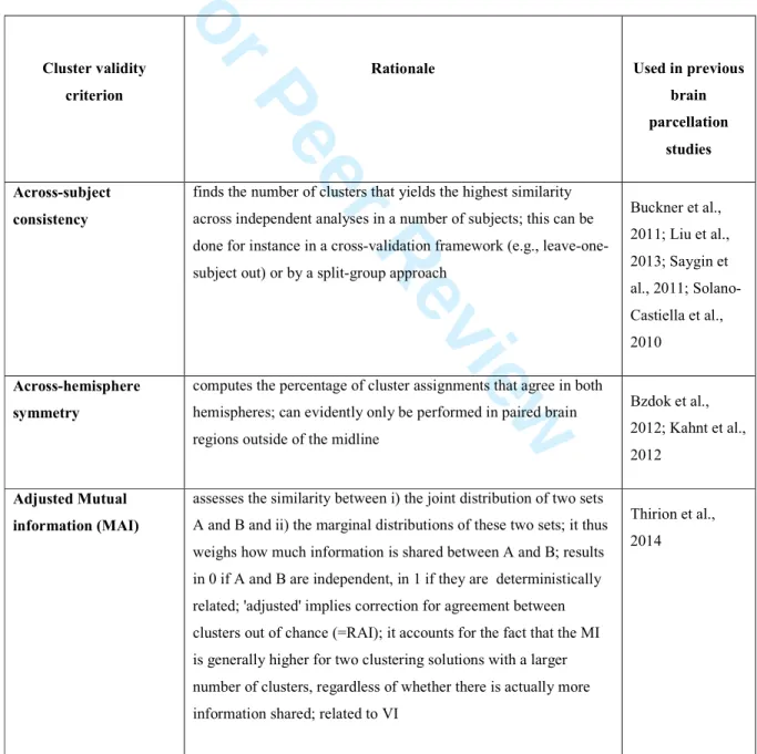
Cluster validity problem. From a broader perspective, the 'true' shape and number of clusters is unknown for
most real-world clustering problems, including brain research. Finding an 'optimal' number of clusters represents an unresolved issue (cluster validity problem) in computer science, pattern recognition, and machine learning (Handl et al., 2005; Jain et al., 1999). This has prompted the development of diverse heuristics (cluster validity
criteria) to weigh the quality of the obtained clustering solutions. These are necessary because clustering algorithms will always find subregions in the investigator's ROI, whether these truly exist in nature or not.
2 3 4 5 6 7 8 9 10 11 12 13 14 15 16 17 18 19 20 21 22 23 24 25 26 27 28 29 30 31 32 33 34 35 36 37 38 39 40 41 42 43 44 45 46 47 48 49 50 51 52 53 54 55 56 57 58 59 60