HAL Id: hal-00622969
https://hal.archives-ouvertes.fr/hal-00622969
Preprint submitted on 13 Sep 2011HAL is a multi-disciplinary open access
archive for the deposit and dissemination of sci-entific research documents, whether they are pub-lished or not. The documents may come from teaching and research institutions in France or
L’archive ouverte pluridisciplinaire HAL, est destinée au dépôt et à la diffusion de documents scientifiques de niveau recherche, publiés ou non, émanant des établissements d’enseignement et de recherche français ou étrangers, des laboratoires
European Cooperative R&D And Firm Performance
Luis Aguiar, Philippe Gagnepain
To cite this version:
Luis Aguiar, Philippe Gagnepain. European Cooperative R&D And Firm Performance. 2011. �hal-00622969�
European Cooperative R&D
And Firm Performance
∗
Luis Aguiar
†and Philippe Gagnepain
‡August 10, 2011
Abstract
The goal of this paper is to assess the impact on the performance of firms that participate in Research Joint Ventures (RJVs) funded by the Fifth European Framework Programme for Research and Technological Development (EU-FP5). A special emphasis is made on the User-friendly Information Society (IST) pro-gramme, one of the most important thematic programmes of the EU-FP5. We use the funding available to the firms as an instrumental variable to account for self-selection and estimate the Local Average Treatment Effect (LATE) of par-ticipation by considering labor productivity and profit margin as performance measures. Our results show a large and positive impact of participation on the labor productivity of the firms, whereas the effect on profit margin is weaker. When taking into account the size of the RJV, we find that the positive impact on labor productivity comes mainly from participation in large projects and that participation in smaller RJVs has a negative effect on the profit margin.
Keywords: Research Joint Venture, R&D policy, Productivity, EU Framework programme.
JEL classification: L24, L25, O31, O32, O38.
∗This paper is produced as part of the CEPR project “SCience, Innovation, FIrms and
mar-kets in a GLObalized World (SCI-FI GLOW)” funded by the European Commission under its Seventh Framework Programme for Research (Collaborative Project) Contract no. 217436. We thank participants at the Universidad Carlos III de Madrid, the 2010 Zvi Griliches Research Seminar in the Economics of Innovation in Barcelona, the 2010 MICRO-DYN conference in Cambridge, the XXV Jornadas de Econom´ıa Industrial in Madrid and the 2011 ENTER Jam-boree Conference in Tilburg. All remaining errors are ours.
†Universidad Carlos III de Madrid. E-mail: [email protected]
‡Paris School of Economics/Universit´e Paris 1 and CEPR. E-mail:
1
Introduction
Research and development (R&D) investments are flawed by two important char-acteristics that make their free-market equilibrium levels less than socially desir-able. First, R&D is non-rival in that the knowledge produced by a firm’s in-vestment does not prevent other firms to access the same amount of information. Second, it is characterized by spillovers: A firm investing in R&D usually imposes a positive externality on the other firms which can appropriate the results of this investment (see De Bondt (1997) for a review).
By and large, two types of public policies are used to try to solve this problem: Direct subsidies and internalization of the externality through research collabora-tion. The former is aimed at modifying the marginal return of R&D investments, while the latter (partially) solves the appropriability problem. Another public policy involves a mix of these two instruments, where the government grants subsidies to a group of firms to encourage them to collaborate within an R&D project or a research joint venture (RJV). This is the type of public policy used by the European Union (EU) in its Framework Programmes (FPs). Since 1984, research and innovation activities from the EU are bundled into the EU-FPs. They have been the main financial tools with which the EU Commission has sup-ported cooperative R&D activities, and the EU participation in the coordination and financing of RJVs has been increasing until today.1
In this paper, we provide empirical evidence on the effect of these FPs on various firm level performance measures such as productivity and profitability.
So far, evaluation studies on these programmes have not really helped under-stand their impact on the competitiveness of European industries. Luukkonen (1998) argues that there are two main reasons to this lack of understanding. The first comes from the general nature of the objectives pursued by the EU Com-mission and the ensuing difficulty in evaluating their attainment. The second concern problems in the evaluation studies themselves, and the fact that they are part of the political process which formulates these programmes, leading to less critical and internal evaluation. Georghiou and Roessner (2000) also point out many difficulties in realizing thorough evaluations of technology programs. Due to the large amount of public funds raised by the EU-FPs and to the potential
1
FP1, FP2, FP3, FP4, and FP5 were allocated 3.75, 5.4, 6.6, 13.2, and 14.960 millions e respectively (see Artis and Nixson (2001)).
problems that RJVs may cause vis-`a-vis European competition policy standards, these results seem rather disappointing.
Some other studies have been carried by academic researchers and have tried to analyze the impact of RJV participation on innovative output, such as sales of innovative products or patenting activity (Branstetter and Sakakibara (1998), Branstetter and Sakakibara (2002), Dekker and Kleinknecht (2008), Czarnitzki, Ebersberger, and Fier (2007)), or on economic performance, as measured by firm productivity or profit margin (Irwin and Klenow (1996), Belderbos, Carree, and Lokshin (2004), Cincera, Kempen, van Pottelsberghe de la Potterie, Veugelers, and Villegas Sanchez (2003), Siebert (1996)). This literature supports a posi-tive relationship between R&D cooperation and innovation but shows less clear results on the impact of collaboration on competitiveness and economic results of the firms. On top of that, the studies concerning the effect of participation in the EU-FP on firm performance are rather scarce. Some exceptions are Ben-fratello and Sembenelli (2002) and Barajas, Huergo, and Moreno (2009). The former analyzes the impact of participation in FP3 and FP4 on productivity for manufacturing firms but find no significant effect. The latter uses a structural approach to estimate the effect of participation in EU-FPs on economic perfor-mance for Spanish firms between 1995 and 2005 (hence covering part of FP4 (1994-1998), all of FP5 (1998-2002) and part of FP6 (2002-2006)). They find a positive impact on the technological capacity of firms (measured by intangible fixed assets, an indirect measure of innovation output), which is positively related to their economic performance, measured by labor productivity.
The Fifth Framework Programme had a budget of EUR 14.96 billion for the period 1998-2002 and is composed of four different thematic programmes. In this paper, we focus on the one that had the largest budget allocation, the User-friendly Information Society (IST) programme, with a budget of EUR 3.6 billion. We analyze it in more detail by looking into its effects on the performance of participating firms. Furthermore, a special emphasis is made on the reforms undertaken by the programme with respect to its predecessors. We take into ac-count the different instruments from the programme (the so-called Key Actions and the various types of contracts offered to participants) to isolate any potential impact on the participants’ economic performance. We take into account and adjust for self-selection of firms into the programme by using instrumental
vari-ables estimation methods. Moreover, our database allows us to introduce a time lag of as much as four years from the start of each project in order to look at the long term effects of participation.
The remainder of the paper is organized as follows. Section 2 summarizes theoretical and empirical literature on the subject. Section 3 presents the struc-ture of the EU-FP5 and its main characteristics. Section 4 presents the data and the construction of the dataset. Section 5 shows some descriptive statistics while section 6 is devoted to the empirical model and the discussion of the estimation results.
2
Related literature
The growth of R&D partnerships observed since the 1980’s has generated an increasing interest in such collaboration activities for both academics and policy makers (Hagedoorn (2002)). A first theoretical approach on the subject is offered by the management and business literature and justifies the creation of R&D collaborative agreements by the opportunity they give to minimize transaction costs and exploit complementary know-how between participants (Kogut (1988)). The second strand of literature comes from the Industrial Organization (IO) theory and focuses on the imperfect appropriability of R&D results presented above.2
The theoretical IO literature has mainly focused on horizontal R&D cooperation (i.e. on the collaboration between firms that are competitors in the product market) and on the impact of these agreements and knowledge spillovers on the incentives to innovate.
The basic theoretical models analyzing RJVs started developing in the mid-1980’s and mainly focus on comparing the welfare implications of R&D coop-eration with the ones of R&D competition (Katz (1986), Spence (1984), and d’Aspremont and Jacquemin (1988)).3
The vast majority of these models con-clude that spillovers have an important role in defining the relative efficiencies of cooperative and non-cooperative scenarios. The effect of a joint venture in R&D is an increase in the profits for both firms (for any spillover value) and an increase
2Hagedoorn, Link, and Vonortas (2000) distinguish between three categories of literature,
dividing the business literature into transaction costs and strategic management literature.
3See also Kamien, Muller, and Zang (1992), Suzumura (1992), Leahy and Neary (1997), and
in R&D investment and welfare if the spillovers are large enough.4
While the theoretical literature on RJVs is substantial, the empirical studies on the subject are rather scarce. The empirical literature can broadly be divided into two categories. The first one consists of papers analyzing the determinants of RJV participation, while the second category analyzes the impact of collaboration on performance. The present paper falls under this last category by trying to as-sess the effects of the European Union Fifth Framework Programme for Research and Technological Development (FP5) on the performance of its participants.
A first set of studies has focused on the determinants of RJV formation and participation. Hern´an, Mar´ın, and Siotis (2003) analyze the determinants of participation in European RJVs and find that sectorial R&D intensity, industry concentration, firm size, technological spillovers, and past RJV participation pos-itively influence the probability of forming RJVs. Mar´ın and Siotis (2008) extend this analysis by exploiting the differences in institutional design of two European collaboration programmes (EUREKA and the EU-FP) and relating them to RJV participants’ characteristics. Firms frequently participating in EU-FP RJVs are primarily large firms in intensive R&D sectors. As pointed by the authors, this might reflect a preference for EU authorities for firms sharing these character-istics, but it may also suggest that an EU-FP RJV is an attractive option for projects involving large R&D outlays because of the cost-sharing element. They also note that past experience in the EU-FPs is an important factor explaining participation. R¨oller, Siebert, and Tombak (2007) find that cost-sharing is an important motive for RJV participation. Moreover, firms asymmetries also plays a key role since similarly sized firms are more likely to form an RJV. Finally, firms are more likely to engage in further RJVs when their participation rate in other RJVs is higher.
The second category of empirical studies analyzes the effect of participation on performance. Branstetter and Sakakibara (1998) and Branstetter and Sakak-ibara (2002) analyze the impact of Japanese government-sponsored research con-sortia on the research productivity of participating firms. It is found that firms which participate in more research consortia do spend more on R&D and that an additional project per year raises a firm’s R&D productivity. The greater
4When firms do cooperate and information leakage is high, they internalize this effect and
increase their R&D investment relative to the non-cooperative scenario. It is important to emphasize that if an RJV is formed in these models, it will always encompass the whole industry.
the potential spillovers within a consortium, the greater the equilibrium level of R&D expenditure by member firms. Moreover, technological proximity has a sig-nificantly positive effect on consortium outcome (i.e., the amount of patenting), while product market proximity has a significantly negative effect on consortium outcome. Finally, another important suggestion of their analysis is that the de-sign of a consortium matters much more than the level of resources expended on it.
Studies trying to measure the impact of cooperation on the economic perfor-mance of firms rather then their innovative perforperfor-mance is quite scarce. An early work analyzing the effect of RJV participation on firm economic performance is the one by Siebert (1996). Analyzing 314 US joint ventures, he shows that cooperation has no direct impact on profit margin, but does increase the effect of R&D intensity on the profit margin. Belderbos, Carree, and Lokshin (2004) study the impact of cooperation on firms’ performance (labor productivity and productivity in innovative sales new to the market) and differentiate between the type of R&D partner (competitors, suppliers, customers, and universities and research institutes). They find that supplier and competitor cooperation has a significant impact on labor productivity growth. Cooperation between firms and universities or research institutes (as well as cooperation with competitors) has a positive impact on growth in sales per employee of products and services new to the market.
Benfratello and Sembenelli (2002) carry an analysis to evaluate the impact of European collaboration programs on participating firms’ productivity (labor productivity, total factor productivity and price cost margin). They study the impact of two different programs, EUREKA and the (3rd and 4th) EU-FPs in the 1992-1996 period. In EU-FP, projects are funded and co-ordinated by the Eu-ropean Commission (top-down structure) whereas EUREKA projects have a de-centralized funding source and research projects are proposed and defined by the participants themselves (bottom-up structure). Hence, the public involvement is larger in EU-FP. The main results of the analysis is that firms participating in EUREKA have experienced a significant improvement in their performance mea-sures. On the other hand, firms participating in RJVs under the EU-FP scheme do not show any significant change in performance.
Dekker and Kleinknecht (2008). Using data from the Community Innovation Sur-vey (CIS) that directly measures innovation, they test the effects of the Program on the participants’ R&D input and innovative output, measured as the sales of innovative products per employee. Their main result is that after correcting for self-selection, participation in the EU-FP does not increase the sales of innovative products. Results also show that there is a significant increase in R&D efforts for small firms who participate in an EU-FP project, while participation by medium and large firms has no significant impact on R&D intensities.
Finally, a recent study by Barajas, Huergo, and Moreno (2009) analyzes the impact of participation in the EU-FP on labor productivity of Spanish manufac-turing firms between 1995 and 2005. Their approach follows the work of Crepon, Duguet, and Mairesse (1998) and considers that participation in the EU-FP has an indirect effect on productivity through the generation of new knowledge. In other words, participation has a positive impact on firms’ technological capa-bilities (captured by intangible fixed assets), which in turn have an effect on firms’ performance, measured by labor productivity. They also use data on ac-cepted and rejected applications to estimate a selection equation to correct for self-selection.
3
The European Union Framework Programmes
The main objective of European policies toward research joint ventures in the beginning of the 1980’s was to fight the relative decline in the international com-petitiveness of high technology sectors. Other factors specific to the European Community (EC) also influenced the need for these policies. For instance, there were large differences between the many country members in terms of indus-trial and technological capabilities. Some members also had an already well established policy infrastructure for Science and Technology while others totally lacked such infrastructures. Finally, there was no appropriate legal framework and institutions at the EC level for supporting a consistent technology policy. In 1981, these considerations led the European Commission to establish the pilot ESPRIT program with the endorsement of the twelve largest European producers of electronics (Hagedoorn, Link, and Vonortas (2000)).
research policy came with the formation of the EU Framework Programme (EU-FP). The First Framework Programme, which started in 1984 and ended in 1987, came in response to a situation where individual R&D activities were uncoordi-nated and required a large number of Council decisions (Georghiou (2001)).
Also at that time arose the formal expression of the policy rationale for the Community action in the field of research and technological cooperation. This is embedded in the principle of subsidiarity, which states that support should come where the scale or cost of cooperation was beyond that affordable by a single country, where complementarily in national work could achieve results for the whole Community, and where research contributes to development of the common market, laws and standards, or to the unification of European science and technology (Georghiou (2001)).
Since 1984, research and innovation activities from the EU are hence bundled into the EU-FP. These have been the main financial tools with which the EU supports R&D activities covering almost all scientific disciplines. Six FPs have already been completed and the seventh has just been started in 2007. Each of these programmes covers a period of five years with the last year of one FP and the first year of the following FP overlapping.5
The aim of these EU-FPs is to support and encourage European research, but the detailed objectives of each programme vary from one funding period to another. All of the RJVs that are formed under this programme are eligible for an EU subsidy, which varies according to the nature of the project. One important characteristic of EU-FP projects is their “pre-competitive” orientation, necessary to avoid conflict with the EU competition law. Defined more precisely, pre-competitive research concerns R&D for which commercial possibilities remain five to ten years in the future (Luukkonen (1998)).
The main objective of the FP5 is to stimulate transnational collaboration in research, particularly between industry and universities, and the establishment of networks of excellence.6
The FP5 comprises four thematic programmes, each addressing a series of scientific, technological and societal issues7
. The four the-matic programmes are (i) Quality of Life and Management of Living Resources
5
The seven FPs cover the periods 1984-1987, 1987-1991, 1990-1994, 1994-1998, 1998-2002, 2002-2006, and 2007-2013.
6
See European Commission (2000) and European Commission (2001).
7
(QUALITY), (ii ) User-friendly Information Society (IST), (iii ) Competitive and Sustainable Growth (GROWTH), (iv-a) Energy, Environment and Sustainable Development (EESD), and (iv-b) Nuclear Energy (EESD/EURATOM). In turn, the three horizontal programmes are (i) Confirming the International Role of Community Research (INCO), (ii ) Promotion of Innovation and Encouragement of Participation of SMEs (INNOVATION & SME), and (iii ) Improving Human Research Potential and the Socio-economic Knowledge Base (HUMAN POTEN-TIAL). In this paper we focus on the most important programme in terms of budget allocation, the User-friendly Information Society (IST) programme.
It is important to note that the European Commission does not itself under-take or participate in the EU-FP projects. Its role is to offer financial or other support to private and public research bodies, and companies and institutions wishing to embark on a research project. Each year throughout the period of the FP5, the commission publishes so-called workprogrammes that contain dif-ferent calls for proposals that describe the objectives planned (Zobel (1999)). The proposal of a project must then be submitted in response to these specific calls. This means that unsolicited project proposals are not allowed and the project’s content must correspond to the objectives set out by the commission. Also, several eligibility criteria must be satisfied by the different partners involved in the project. One of them is that the project must involve at least two legal entities (e.g. individuals, industrial and commercial firms including SMEs, uni-versities, research bodies, technology dissemination bodies) independent of each other and established in two different Member States or in a Member State and an associated country.8
The financial contribution from the Commission consists in the reimbursement of a set percentage of the participants’ eligible expenses, although sometimes flat-rate contributions are made. In order to be reimbursed by the Commission, participants must identify and report their eligible expenses by submitting interim and final statements. In particular, the expenses must be necessary for the action in question, provided for in the contract, actually incurred and recorded in the accounts. Finally, it is important to note that participants cannot establish intellectual property rights over their discoveries: all research must be shared
8This means that entities established outside the EU and international organizations can
among partners.
4
Data and variables
The empirical analysis will be carried out using a database constructed from two different sources. The data from the EU-FP projects will first be taken from the Community Research and Development Information Service (CORDIS) web page. We will focus on the projects involved in the User-friendly Information Society (IST) programme. Available on the CORDIS web page is a total number of 2522 projects.9
The second source of information is the one about the participating firms. Once the information about each project is recovered, we can look at each par-ticipating firm individually and obtain firm-level data. This latter task will be done using Amadeus (Analyse MAjor Databases from EUropean Sources), a data base produced byBUREAU Van DIJK, a specialist provider of firm-level data. The final data set is constructed using the information from the two sources presented above. Firms participating in projects recovered from the CORDIS web page are linked to the Amadeus database in order to retrieve the relevant information at the firm-level. The Amadeus database contains balance sheet information on the top 250,000 firms in Europe. The CORDIS database provides information on each project, i.e. its description, its reference, the starting and ending dates of the project, its status and its acronym, the contract type offered to the participants, the cost of the project as well as the funding provided by the European Commission. The name of the coordinator of the project and of the participating firms are given as well.
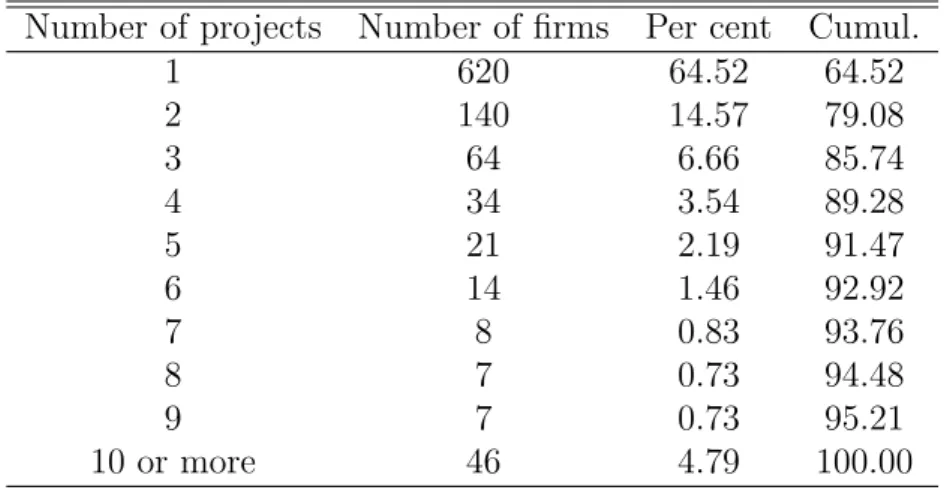
We were able to retrieve 961 firms that participated in at least one FP5 RJV from Amadeus. Table 1 gives the different number of RJVs the firms participate in and shows how some firms were often involved in more than one project. We decided to focus on the firms that participate in one project only. This corresponds to a total of 620 firms participating in 466 projects. After cleaning the dataset, we end up with a total of 379 participants that correspond to 315 projects.
5
Descriptive Statistics
We present some descriptive statistics of the constructed database. We first describe the main characteristics of the EU-FP5 projects before turning to the description of the participating firms.
5.1
Projects description
Table 2 presents some average values for the projects included in the database. The column All Projects represents all the projects we could recover from the CORDIS webpage for the EU-FP5 (2359 projects), while the column Single Part contains the projects in which only single participants (in our data set, that is) are involved (466 projects). The last column Sample contains information on the projects that correspond to the participating firms present in our final sample (315 projects). The projects that we are able to analyze seem to be larger in terms of number of participants and cost. Unless otherwise stated, the next tables will present statistics of the projects included in our final sample.
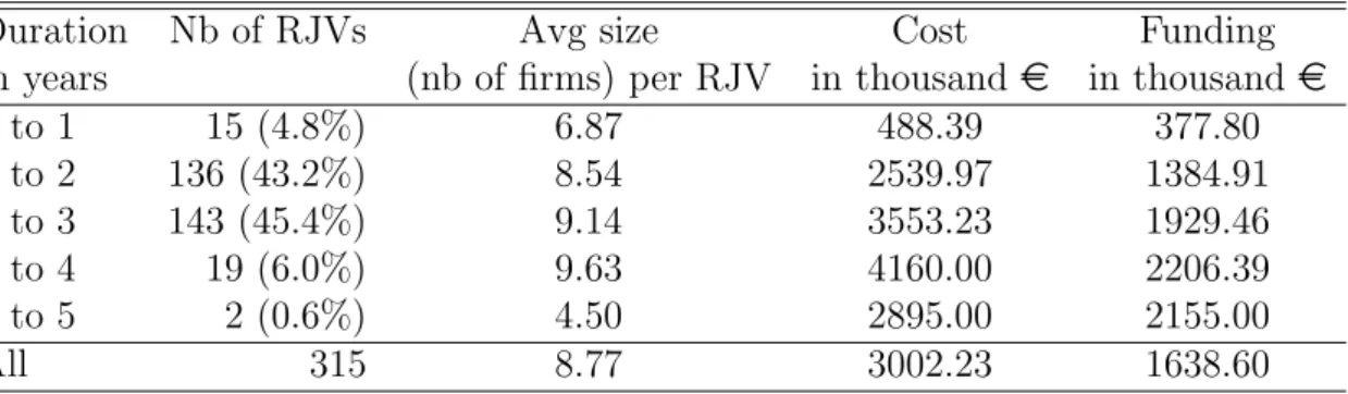
Table 4 provides summary statistics on the number of participants by project. We can see that the projects are more or less evenly distributed, with a higher proportion incorporating 6 to 10 participants. The duration is on average lower when projects have few participants (0 to 3) and the cost of each RJV is increasing with the number of participating firms. Concerning the cost of the different projects, table 5 reveals that the majority of RJVs have costs between 0 and 6 millions euros, with a peak for the ones with costs between 1 and 3 millions. Finally, table 6 shows that the vast majority of the RJVs last from 1 to 3 years.
5.2
Comparison of Amadeus and Participants
In this section we look at the characteristics of the participants that are included in our database. We first compare them with the overall Amadeus database in order to see if there are some important differences. Indeed, one important prob-lem one has to deal with when evaluating the impact of government-sponsored R&D is the one of selection bias since it is hard to think of RJV participation as being randomly assigned or decided. This inevitably creates a potentially im-portant bias in the estimated impact parameters (Klette, Moen, and Griliches
(2000)).
We give a first look at this potential selection problem by comparing basic statistics. Table 7 gives summary statistics on some variables for both the par-ticipants and non-participating firms in Amadeus for 1999. Parpar-ticipants have significantly larger figures for most of the variable considered, confirming the fact that the programme selects larger firms for participation. Further evidence of this fact is given in figure 1, which shows the distributions of the log transformation of sales, employees and fixed assets for both participants and firms contained in Amadeus. In all cases the participants’ distribution is similar to the one of the outsiders, only shifted to the right.
6
Empirical model
To perform our empirical test, we use three different samples. The first one is composed of the participating firms and of non-participating firms randomly picked from Amadeus. After cleaning the data, we are left with 2134 observa-tions for participants and 6638 for the selected non-participants over the years 1997 to 2006. This sample is referred to as the Random sample throughout the text. As in Benfratello and Sembenelli (2002), the alternative control group used in our estimations is constructed by selecting non-participating firms from Amadeus so as to replicate the cross-tabulation of participants by country and industry. After cleaning the data, we are left with 2134 observations for partici-pants and 3531 for the selected non-participartici-pants over the years 1997 to 2006. In our estimations, we call this sample IC-Rep (for Industry Country Replication). Last, we use a third control group constructed so as to replicate the distribution of the sales variables of the participants for 1999 (i.e. before the start of any project). The final kernel density estimates of the control group for 1999 are presented in figure 1. After cleaning the data, we are left with 2134 observations for participants and 3726 for the selected non-participants over the years 1997 to 2006. We call this sample Sales-Rep in our estimations.
We provide an empirical test on the effect of participation in the User Friendly Information Society programme of the EU-FP5 on the firms’ performance. The performance measures that will be considered are labor productivity, measured as added value per employee, and profit margin, measured as the profit
(be-fore taxation) over the operating revenue. In what follows we will use the term performance to denote either of these two measures.
Let Pit = 1 be the event of firm i participating in a project at time t and let
yit be the measure of firm i’s performance. Denote by y0it and y 1
it the performance
of firm i at time t when it does not and when it does participate in EU-FP5 respectively. Hence we write
yit= { y1 it if Pit = 1 y0 it if Pit = 0.
Equivalently, yit can be expressed as
yit = y 0 it+ (y 1 it− y 0 it)Pit. (1)
We want to know the effect of participation at time t on the firm’s performance yit. This effect can be expressed as ∆it ≡ yit1 − y
0
it. It measures the difference
between the observed performance of participant i and the performance it would have reached had it not participated in the project. Since the counterfactual out-come y0
it can never be observed for a participating firm, ∆it cannot be computed
directly and needs to be estimated. If we consider a constant treatment effect, i.e. ∆it = yit1 − y
0
it = δ, we can rewrite (1) as
yit = α + δ · Pit+ εit, (2)
where εit is an error term. A direct approach to circumvent the missing
coun-terfactual problem is to replace the missing councoun-terfactual outcome by the mean performance of the non-participating firms. This would be a simple treatment-control comparison (TCC) estimator as it mimics the analysis in an experimental setting. The estimator of δ, bδT CC, would then be the mean difference in
perfor-mance between participants and non-participants.
At this point, it is important to clarify the definition of the participation dummy variable Pit. Notice that we have so far assumed that Pit = 1 if firm i
participates in an RJV at time t. However, it may well be that this firm had been involved in the project for several periods prior to t. But the point is whether firm i is currently involved in an RJV at time t. Notice, however, the drawback of this definition for the participation dummy. Firm i may be considered
non-participant at time t if it is not involved in any project at that time (i.e. Pit = 0)
although it may have participated in a project prior to t. This suggests another definition of participation. We will create the dummy PARTSit that takes the
value one from time t onwards if firm i was involved in an RJV at time t and 0 otherwise. In other words, we have that PARTSit = 1 if firm i has already
entered or is currently participating in a project at time t, whereas PARTSit = 0
if firm i has not entered any project at time t yet. It follows that the coefficient on this new dummy has now to be interpreted as the effect of participating (or having participated) in a project on the mean productivity compared to a firm that is not participating in any project.
A simple treatment-control comparison in the form of equation (2) is most likely to yield inconsistent estimates. As mentioned above, bδT CC will suffer from
a selection bias since it is hard to think of participation into the EU-FP5 as being random. Selection bias comes from the existence of firms’ characteristics (be they observable or not) that are correlated with participation in the programme. To the extend that the programme attracts bigger and more productive firms, we have to deal with a positive selection bias. We therefore also control for observable characteristics x that affect both the decision to participate (treatment) and the productivity of the firm (outcome). Doing so leads to the following specification: yit+τ = x′itβ+ δτ · PARTSit+ εit+τ. (3)
Estimation of δ from equation (3) allows to control at least for selection on observable characteristics. Size effect is controlled for by including in vector x the log of employees. Also included in x are the ratio of tangible fixed assets over employees (in logs) as a proxy of physical capital intensity and the ratio of intan-gible fixed assets over employees (in logs) as a proxy of knowledge capabilities. We also include as an explanatory variable the total number of partners with which a firm collaborates within a given project. Finally, a set of 2-digit industry dummies, grouped into 19 industries, as well as country and time dummies are included to control for industry, country and time effects.
Columns (OLS) of tables 11 and 12 show the results of estimating (3) by pooled OLS for years 2000 to 2006. In table 11, the dependant variable is the logarithm of labor productivity, while in table 12 the dependant variable is the profit margin. The results show that the average impact of participation on labor
productivity is positive and significant, whereas the effect on the profit margin shows up to be non significant and rather small.
The estimation strategies presented above allowed to solve for the selection problem to the extend that firms self-selected in the programme based on some observable characteristics we could control for. However, if firms decide on par-ticipation based on unobservable characteristics included in εit, the endogeneity
problem will remain and estimators will still be inconsistent. In our case it is most likely that firms do in fact decide on participation based on some unobservable characteristics. For example we can think of firms as having some “managerial” or “innovative” ability that may influence on their decision to participate in an RJV. One possibility to overcome this issue is to take advantage of the panel structure of our data to allow for possible time-invariant unobservable firm char-acteristics that may influence participation in the programme. Assuming that the unobserved characteristics in (3) can be decomposed as εit = ηi+ uit allows
for correlation between the participation variable PARTSitand the time-invariant
firm specific effect ηi. This leads to the following specification
yit+τ = x′itβ+ δτ · PARTSit+ τt+ ηi+ uit+τ, (4)
where uit is an i.i.d. zero mean random variable assumed to be uncorrelated
with xit and the time effects τt have now been made explicit.
We can use fixed-effects estimation to obtain a consistent estimator of δ in (4) provided the participation dummy, PARTSit, is strictly exogenous. We hence
need that COV(uis,PARTSit) = 0 for any t and s. Tables 8 and 9 show the
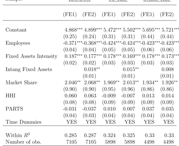
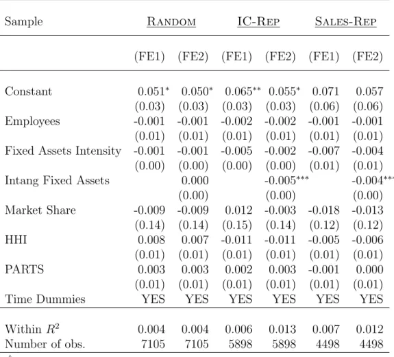
results of the fixed-effects estimation of (4) using data pooled over the years 2000 to 2006. The results now show an average effect of participation that is close to zero and non significant on both of our performance measures. Hence we have that when controlling for self-selection (and assuming that the latter is based on unobservable characteristics that remain constant over time) participation has, on average, no effect on the economic performance of the firms. These results are in accordance with the results of the previous literature that we presented above.10
10Note that the necessary condition for the consistency of the fixed effects estimator is likely
to be violated if programme participation changes in reaction to past outcomes of yit. In this
case, we have that COV(uis,PARTSit) ̸= 0 for s < t. Klette, Moen, and Griliches (2000) give
In the next section we turn to an instrumental variables estimation strategy to circumvent the self-selection issue.
6.1
Instrumental Variables estimation
Estimation by instrumental variables requires finding a variable (the instrument) that determines programme participation (i.e. that is correlated with PARTSit)
and that is uncorrelated with the error term εit. The empirical strategy is then
to estimate the impact of participation in two steps. We first need to specify an equation explaining the participation decision. In particular, we assume that the probability that firm i decides to engage in an RJV is given by
Pr(PARTi = 1 | z) = F(zit′ γ). (5)
The variables in the vector x in (3) are a subset of the variables in z. That is, at least one element of z (call it z1) is unique and is a non-trivial determinant
of PARTi. Hence z1 is an instrument correlated with the endogenous dummy
variable PARTit but that has no direct effect on the outcome yit (it only has an
effect through PARTit). We will specify F (·) to be the cumulative distribution
function of the logistic distribution and hence estimate (5) by logit. The first step of the estimation consists in estimating (5) in order to obtain the predicted values \PARTi. The second step uses these predicted values to run regression (3).
We use the following variables to explain the participation decision into the programme. We first account for the logarithm of employees, which is used as a measure of firm size. This variable may have an important effect on participation in case specific fixed costs for the creation of an RJV exist. We also introduce as an explanatory variable the ratio of tangible fixed assets over employees (in logs) as a proxy of physical capital intensity. Another variable that may influence the willingness to participate in an RJV is the relative size of the firm within the industry in which it operates. As noted by Hern´an, Mar´ın, and Siotis (2003), relative size may matter if RJVs are used as a vehicle for pursuing “technology watch”, i.e. to monitor innovative activity in their segment. As they point out, the largest firms (which are also the technology leaders), have most to lose from
large firms facing severe problems when the IT industry was restructured towards the end of the 1980’s. In such case, the fixed effects estimator above would underestimate the impact of participation on the participants.
the emergence of new, technologically advanced rivals (see also Laredo (1998)). This measure is proxied by the introduction of a variable measuring market share, calculated as firm size over industry size, both measured by the amount of sales.11
One main shortcoming of our dataset is the unavailability of R&D expenses at the firm level. In order to overcome this problem, we use the ratio of intan-gible fixed assets over employees (in logarithm) as a measure of the intensity of the firm’s innovative activity. In any case, this variable is likely to be highly correlated with a firm’s “absorptive capacity”, increasing the likelihood of par-ticipation in an RJV. A measure of industry concentration is also included with the Herfind¨ahl-Hirschman Index (HHI).12
This indicator can have an ambigu-ous effect on participation. A highly concentrated industry can facilitate the identification of suitable partners and spillovers to non-participants are limited because of their reduced number. Also, an RJV may well be created in order to weaken competition or increase the market power of its participants, in which case concentration would increase the likelihood of RJV participation. However, strict limits are imposed on collaborative projects in concentrated industries by competition policy.13
Country dummy variables as well as industry dummies are included in the analysis. Last, we use the funds available for each firm as an exogenous variable to explain participation. The budget dedicated to R&D (through the funding of RJVs) for, say, industry i is likely to be correlated with the participation decision of firms from this same industry. A firm will be more willing to participate if it knows that more funding is available, and the commission will also be more likely to accept a project if it has more funding to offer. On the other hand, the budget is unlikely to be correlated with the unobserved variables affecting labor productivity of the firm and willingness to participate in the programme since its allocation is not made as a function of the participants or potential participants14
. This instrumental variable was first used by Lichtenberg (1988) to identify the
11
This index is constructed over the entire Amadeus database at the 4-digits industry level.
12Similarly to our market share measure, this index is constructed over the entire Amadeus
database at the 4-digits industry level.
13An example is the EU’s block exemption which automatically allows ventures between
firms that collectively represent less than 25% of the relevant anti-trust market but requires authorization for values above that threshold.
14This remark is drawn from discussions with the programme’s managers at the European
effects of “procurement by design and technical competition” contracts on firms’ R&D investments. It has to our knowledge never been used in the analysis of the EU-FPs nor in the context of RJV studies. To construct the variable representing the “available funding”, we first sum the funding received by all the participating firms in a given industry (defined at the 4-digit level). Hence the funding available to industry i is given by the following expression:
AVFUNDi =
∑
RJVj
dij · Fundingj,
where dij is a dummy equal to 1 if the a firm from industry i participates in
RJV j, and Fundingj is the funding received by RJV j from the commission.
With these covariates properly defined, we can now rewrite equation (5) as
Pr(PARTi = 1 | z) =F(z′itγ) =F ( γ0+ γ1log(Employees)it+ γ2log (FixedAssets Employees ) it +γ3log (IntangibleAssets Employees ) it+ γ 4HHIit+ γ5MktShareit +γ6log(AvailableF unding)i + C ∑ c=1 θcCountryic+ J ∑ j=1 φjIndustryij + 99 ∑ s=98 λsdst ) . (6)
Our strategy is to use pre-determined observations to explain programme participation in order to mitigate further endogeneity issues. For this purpose, we use observations for years 1997 to 1999 to estimate equation (6). Table 10 presents the results of the logit estimation of equation (6). We present two alternative specifications in order to assess whether the results are sensitive to the exclusion of intangible assets as a determinant of participation. The coefficient on our instrumental variable turns out to be positive and strongly significant in both specifications, corroborating the fact that the available funding is indeed an important predictor of participation in the programme.
The market share variable, measuring firms’ relative size, is positive and signif-icant in all the specifications. This is in accordance with the “technology watch”
explanation presented above, which suggest that relatively large firms in their industry (i.e. leaders) may have an incentive to participate in the programme to monitor the innovative activity in their segment.
Although significant in only two of the samples, the HHI variable shows a positive impact on the probability of participation, indicating that firms coming from more concentrated (or less fragmented) industries are more likely to partic-ipate. As argued above, this result is consistent with the fact that firms find it easier to identify suitable partners in such industries. Also, the latter give greater scope for the internalization of spillovers.
The coefficient associated with employees, a measure of firm size, is positive and highly significant when the IC-Rep and Random samples are used15
. As noted in Hern´an, Mar´ın, and Siotis (2003), this indicates that absolute firm size is an important determinant of programme participation and may reflect the ex-istence of large fixed costs associated with RJV formation (for example large administrative and negotiation efforts necessary to reach agreements with part-ners). It may also be the result of certain preferences for large firms from the EU-FP5 organization. The fixed assets intensity, a measure of capital intensity, is a positive predictor of participation, but turns out do be significantly so in the Random sample only, when the intangible fixed assets intensity is not included as a regressor (specification (1)). When the latter is included, its corresponding coefficient is positive and significant, showing the important correlation between the fixed assets and intangible fixed assets variables. Although the coefficient on the intangible assets intensity variable actually shows up to be positive and significant for the Random sample only, it is still positive for our two other sam-ples. This reflects the fact that R&D activities and the absorptive capacity of a firm are important determinants of programme participation.
In the second step of our procedure, we replace the participation dummy by the predicted values obtained in the first step. We use observations from years 2000 to 2006 to estimate the impact of participation on the firms’ performance. Before turning to the discussion of the results, it is important to recall the in-terpretation that must be given to the instrumental variable estimates in our setting. The availability of an instrumental variable allows to identify the
av-15This coefficient is not significant for the Sales-Rep sample given that we constructed it
erage treatment effect (ATE) on the participants (the treated) if our constant treatment effect assumption holds true. In the case where the treatment effects are actually heterogeneous, the instrumental variable is not enough to identify a causal effect on the treated, but identifies instead the local average treatment effect (LATE) as proposed by Imbens and Angrist (1994). The LATE is the av-erage treatment effect for the firms whose treatment status (participant or not) is influenced by changes in the instrumental variable (the so-called compliers). For the LATE to be identified, an additional monotonicity assumption still needs to be met. This assumption essentially says that the instrument must affect the participation decision in a monotone way: if, on average, participation is more likely given a value of the instrument Z = w than given Z = z, then any firm who would participate given Z = z must also participate given Z = w. In our setting, this means that a participating firm facing a given value of available funding would still be willing to participate if it were facing a larger amount of funding. This assumption is likely to hold in our context. Our results should therefore be interpreted as the average impact of the programme for those firms induced to participate as a result of the change in the funding available to them. In other words, they present the average effect of the programme for the subpopulation of “marginal” participants. Although the identification of this subpopulation may not be straightforward, we believe that having a consistent estimate of the LATE parameter is relevant for our purposes. In particular, since our instrument (the available funding) is itself a policy variable, it can be used to implement policy changes that may be suggested by our results.
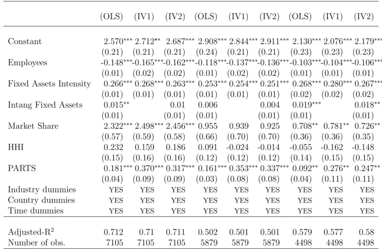
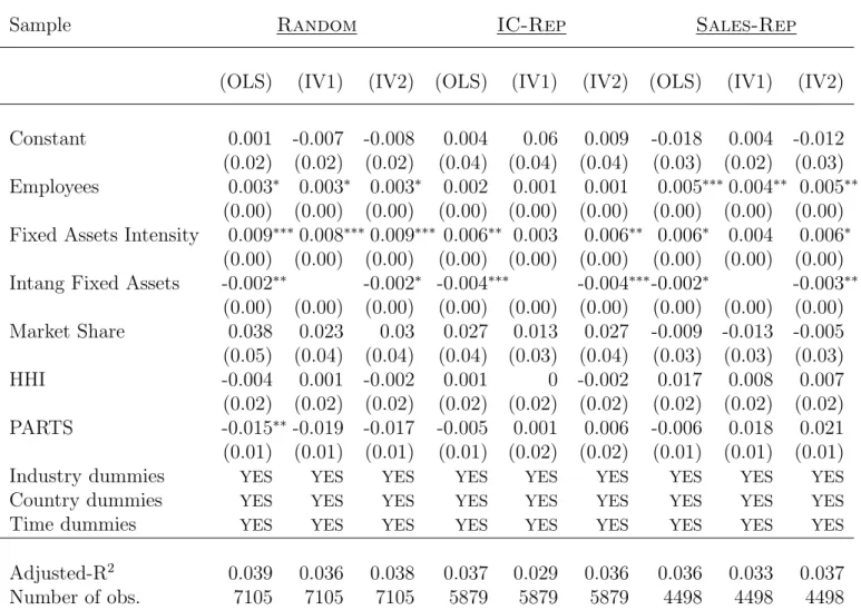
Columns (IV1) and (IV2) of tables 11 and 12 show the results of estimating (3) replacing the participation dummy variable by its predicted value from the corresponding first stage logit estimation in table 10. Concerning the impact of participation on labor productivity, we find that the instantaneous effect is positive and significant. For the firms at the margin of participating, engaging in a RJV from the IST programme raises labor productivity in about 25 to 34%, while it shows no significant impact on the profit margin
Given the pre-competitive nature of EU-FP5 projects, the positive instanta-neous effect presented above may actually be the immediate result of the funding received16
. We therefore also analyze the effect of participation on performance
in the subsequent years after entering a project.
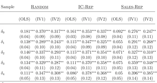
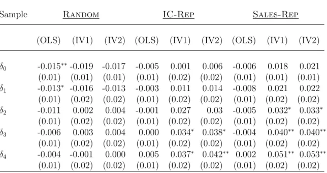
The results are presented in tables 13 and 14 for lagged effects up to 4 years. When considering labor productivity as a performance measure, the coefficients show that participation in the programme has a positive and significant impact up to 4 years after entering a project and accounts for increases in productivity in roughly 31 to 38%. Although no effects were found for the instantaneous effects on the profit margin, our results show that participation leads to an increase of 4 to 5 percentage points three to four years after entering the project (although this result holds in two of our three samples).
6.2
Analysis by RJV size
The results presented in the previous section showed a positive effect of partici-pation on the performance of the firms. Given that the RJVs present in our data set are quite heterogeneous in terms of total cost/funding, it is interesting to see if these gains in productivity are associated with the size of the project in which each firm participates. A first step is to estimate the effect of participation using pooled OLS on the following specification:
yit+τ = x′itβ+ δ L
τ · PARTSLit+ δτS· PARTSSit+ εit+τ, (7)
where PARTSLit = 1 if firm i has already entered or is currently participating
in a large (L) project and PARTSSit = 1 if firm i has already entered or is
currently participating in a small (S) project. We define a large RJV as being one with a total budget of more than 2.8 million euros, which is the median value of the distribution of the projects’ cost in our sample. The vector x includes the same covariates as in equation (3). Columns (OLS) of tables 16 and 17 show the results of running pooled OLS for years 2000 to 2006 on 7 for, respectively, labor productivity and profit margin as outcome measures.
Since the size of the RJV is also the result of a decision made by the partners in the project, one must take this endogeneity into account. To this end, we next use our instrumental variables approach to estimate the effect of participation in the two different kinds of RJVs. Our strategy is similar to the one we followed
by most empirical analysis (see Dekker and Kleinknecht (2008), Benfratello and Sembenelli (2002), Barajas, Huergo, and Moreno (2009)).
in section 6.1 and still consists of two steps. However, we now want to specify an equation that explains participation in the two different types of projects. Each firm i can therefore choose among three alternatives: participate in an large project, participate in a small project or participate in neither of them (i.e. stay out of the programme). We define the dependant variable PARTic to take value
1 if project c is ever chosen, where c = Large, Small, Out. We now specify the following model for the probability that firm i chooses project c,
Pr(PARTic= 1 | z) =F(zit′ γ) =F ( γ0+ γ1log(Employees)it+ γ2log (FixedAssets Employees ) it +γ3log (IntangibleAssets Employees ) it+ γ 4HHIit+ γ5MktShareit +γ6log(AvailableF unding)i + C ∑ c=1 θcCountryic+ J ∑ j=1 φjIndustryij + 99 ∑ s=98 λsdst ) . (8)
where F(·) is the multinomial logistic cumulative distribution function. The multinomial logit estimation is again done using the pre-programme observations (t = 1997, 1998, 1999) to mitigate endogeneity issues. The two specifications we estimate are the same than the ones we used in section 6.1, and the results are presented in table 15.
In the first specification (first part of the table), the intangible fixed assets intensity is left out of equation (8). The coefficient on our instrumental variable is again positive and strongly significant for both small and large RJVs and in both specifications. Almost all of the remaining explanatory variables have the same sign as in our simple logit model. The coefficient associated with employees is strongly significant (except for the Sales-Rep sample, see footnote 15) in predicting participation in both types of RJVs. Capital intensity is a positive predictor of participation, and always a more important one for larger projects. Although not significant, it even shows to be negative for small projects in two of our samples. On the contrary, the intangible assets intensity is a stronger positive predictor for participation in smaller project, although only significantly
so in the Random sample. Firms’ relative size is again positively related to participation, but is significant only for the larger RJVs. This again corroborates our “technology watch” interpretation and further suggests that for a leading firm, monitoring the innovative activity in its sector is more relevant when the projects are of an important size. These kinds of projects are indeed the ones where competing firms could gain the most and take the technological lead. Finally, the HHI index still has a positive sign for both large and small projects and is only significant for one of our samples.
In the second step of our procedure, we replace the participation dummies by the predicted values obtained in the first step. We again use observations from years 2000 to 2006 to estimate the impact of participation in both types of RJVs on the firms’ performance. Tables 16 and 17 show the estimation results for re-spectively labor productivity and profit margin as dependent variables. Columns (IV1) and (IV2) present the results of estimating (7) and replacing the partic-ipation dummy variables by their predicted values from the corresponding first stage multinomial logit estimation in table 15.
We observe that the instantaneous impact of participation is quite different for large and small projects. The positive and significant effect of participation on labor productivity found above seems to come mainly from participation in the large RJVs. For the IC-Rep and Sales-Rep samples, the impact of partic-ipation is actually much lower for small projects than for large ones and is not statistically different from zero. For the impact on profit margin, the results show that participation in small projects leads to lower performance than participation in large RJVs.
These results are confirmed when turning to the lagged effects of participa-tion in the different types of RJVs. Our Random sample did not show a clear difference between the instantaneous effect on labor productivity of participation in large and small projects. However, the lagged effects present a stark difference between the two in all of our samples. The results are presented in table 18 and show important gains on labor productivity (up to 60%) from participating in large projects. Table 19 presents the results when performance is measured by the profit margin. The pattern appears to be clearer than for the instan-taneous effects and reveals a positive (although not always significant) impact from participating in large RJVs, especially starting 2 years after entering the
project. Participation in large projects leads to increases in as much as 8 per-centage points, while participation in small projects leads to decreases to up to 6 percentage points in one of our samples.
7
Conclusion
In this paper we analyze the effects of R&D collaboration within the Fifth Eu-ropean Framework Programme for Research and Technological Development on firms’ performance.
Previous literature has shown that participation in RJVs supported by the EU-FP has no relevant impact on firms’ economic performance, a fact mainly ex-plained by the pre-competitiveness of the programme and its non market-oriented projects. By concentrating on the IST programme, we focus our analysis on the most industry-driven projects, which are likely to be closer to the market than the average EU-FP5 project. We further circumvent the self selection problem using the funding available to the firms as an instrumental variable and esti-mate the Local Average Treatment Effect (LATE) of participation on the labor productivity and profit margin of the firms.
Our results show that participation raises labor productivity by almost 40% three to four years after entering the project, while participation in large RJVs raises labor productivity by up to 60%. We also find a positive effect of par-ticipation on the profit margin three to four years after entering an RJV, with participation leading to an increase of 4 to 5 percentage points three to four years after entering the project. These results hold mainly for large projects though, and we find that participation in small RJVs actually decreases the profit margin by up to 5 percentage points.
Although these estimates might sound surprising given previous studies’ re-sults, it is crucial to recall the interpretation that they must be given. The LATE is the average treatment effect for the firms whose treatment status (par-ticipant or not) is influenced by changes in the instrumental variable, and our results should therefore be interpreted as the average impact of the programme for the subpopulation of “marginal” participants. Even though the identification of this subpopulation may not be straightforward, we believe that our results are economically and policy relevant since our instrument (the available funding) is
itself a policy variable. According to our estimations, raising the available fund-ing would encourage the participation of certain firms that would greatly benefit from it.
8
Appendix
8.1
Tables
Table 1: Number of Projects per firm
Number of projects Number of firms Per cent Cumul.
1 620 64.52 64.52 2 140 14.57 79.08 3 64 6.66 85.74 4 34 3.54 89.28 5 21 2.19 91.47 6 14 1.46 92.92 7 8 0.83 93.76 8 7 0.73 94.48 9 7 0.73 95.21 10 or more 46 4.79 100.00
Table 2: Mean statistics by project
Variable All Projects Single Part Sample Nb of Participants 7.00 8.58 8.77 Duration (in months) 27.04 27.93 27.4 Cost (thousand e) 2376.54 2999.21 3002.23 Funding (thousand e) 1380.21 1663.37 1638.60 Nb of Projects 2359 466 315
Table 3: Projects’ characteristics by starting year
Starting Nb of RJVs Avg size Duration Cost Funding Year (nb of firms) per RJV in months in thousand e in thousand e 2000 96 (30.5 %) 8.23 27.55 3096.99 1683.81 2001 108 (34.3 %) 8.69 27.62 2761.45 1502.80 2002 104 (33.0 %) 9.33 26.68 3240.63 1786.52
2003 7 (2.22 %) 9.29 32.57 1875.71 916.29
All 315 8.77 27.40 3002.23 1638.60
Table 4: Projects’ characteristics by number of participants Nb of participants Nb of RJVs Duration Cost Funding
in months in thousand e in thousand e 3 or less 14 (4.4 %) 17.21 631.56 444.35 4 to 5 36 (11.4 %) 28.19 2429.06 1345.53 6 to 7 89 (28.2 %) 27.94 2657.61 1476.00 8 to 10 105 (33.3 %) 27.12 2874.11 1581.15 11 to 15 48 (15.2 %) 29.25 4163.96 2167.86 16 or more 23 (7.3 %) 27.65 4836.39 2611.22 All 315 27.40 3002.23 1638.60
Table 5: Projects’ characteristics by cost
Cost Nb of RJVs Duration Avg size Funding in millions in months (nb of firms) per RJV in thousand e
0 to 1 53 (16.8%) 18.49 6.68 430.35 1 to 3 122 (38.7%) 28.35 8.13 1191.41 3 to 6 111 (35.2%) 29.91 9.33 2145.41 6 to 8 21 (6.7%) 30.48 13.00 3394.76 more than 8 8 (2.5%) 29.00 13.63 4821.25 All 315 27.40 8.77 1638.60
Table 6: Projects’ characteristics by duration
Duration Nb of RJVs Avg size Cost Funding in years (nb of firms) per RJV in thousand e in thousand e
0 to 1 15 (4.8%) 6.87 488.39 377.80 1 to 2 136 (43.2%) 8.54 2539.97 1384.91 2 to 3 143 (45.4%) 9.14 3553.23 1929.46 3 to 4 19 (6.0%) 9.63 4160.00 2206.39 4 to 5 2 (0.6%) 4.50 2895.00 2155.00 All 315 8.77 3002.23 1638.60
Table 7: Comparison of participants and Amadeus for 1999 Participants Amadeus
Mean Median N Mean Median N Sales 1,617,717.1 61,192.0 560 76,461.5 12,648.0 91475 Employees 7,833.5 441.0 522 482.4 87.0 102273 Fixed Assets 1,295,842.3 15,400.5 598 60,009.1 2,112.0 146753 Intangible Fixed Assets 147,837.6 381.5 582 5,413.6 2.0 140781 Labor Productivity 317.9 63.2 380 141.7∗∗ 49.0 71872
Costs of Employees 366,136.9 20,507.0 508 14,431.1 1,882.0 106638 Mean Wage 49.6 42.5 448 57.5∗∗∗ 31.1 91759
Profit Margin 5.8 4.9 560 5.0∗∗∗ 3.0 124496
Gross Profit Margin 40.1 35.9 140 69.0∗∗∗ 18.3 42718 ∗∗Cannot reject the null hypothesis (equality of the means) in a two-tailed t-test at the 5% level
between the participants and the corresponding control group in each column.
∗∗∗Cannot reject the null hypothesis (equality of the means) in a two-tailed t-test at the 10% level
Table 8: Fixed Effects estimation results: Labor productivity†
Sample Random IC-Rep Sales-Rep
(FE1) (FE2) (FE1) (FE2) (FE1) (FE2) Constant 4.868∗∗∗4.899∗∗∗5.472∗∗∗5.502∗∗∗5.695∗∗∗5.721∗∗∗
(0.25) (0.24) (0.31) (0.31) (0.44) (0.44) Employees -0.371∗∗∗-0.368∗∗∗-0.424∗∗∗-0.424∗∗∗-0.423∗∗∗-0.423∗∗∗
(0.04) (0.04) (0.05) (0.05) (0.06) (0.06) Fixed Assets Intensity 0.187∗∗∗0.177∗∗∗0.178∗∗∗0.169∗∗∗0.178∗∗∗0.173∗∗∗
(0.02) (0.02) (0.03) (0.03) (0.03) (0.03) Intang Fixed Assets 0.018∗∗ 0.015∗∗ 0.008
(0.01) (0.01) (0.01) Market Share 2.046∗∗ 2.068∗∗ 1.969∗∗ 2.013∗∗ 1.934∗∗ 1.926∗∗ (0.90) (0.90) (0.95) (0.96) (0.86) (0.86) HHI 0.060 0.063 -0.009 -0.007 0.013 0.014 (0.08) (0.08) (0.09) (0.09) (0.09) (0.09) PARTS -0.031 -0.037 0.010 0.007 0.037 0.035 (0.04) (0.03) (0.04) (0.04) (0.04) (0.04) Time Dummies YES YES YES YES YES YES Within R2
0.285 0.287 0.324 0.325 0.33 0.33 Number of obs. 7105 7105 5898 5898 4498 4498
† Standard errors in parenthesis. ∗ Significant at the 10% level. ∗∗Significant at the 5% level. ∗∗∗Significant at the 1% level.
Table 9: Fixed Effects estimation results: Profit margin†
Sample Random IC-Rep Sales-Rep
(FE1) (FE2) (FE1) (FE2) (FE1) (FE2) Constant 0.051∗ 0.050∗ 0.065∗∗ 0.055∗ 0.071 0.057
(0.03) (0.03) (0.03) (0.03) (0.06) (0.06) Employees -0.001 -0.001 -0.002 -0.002 -0.001 -0.001 (0.01) (0.01) (0.01) (0.01) (0.01) (0.01) Fixed Assets Intensity -0.001 -0.001 -0.005 -0.002 -0.007 -0.004 (0.00) (0.00) (0.00) (0.00) (0.01) (0.01) Intang Fixed Assets 0.000 -0.005∗∗∗ -0.004∗∗∗
(0.00) (0.00) (0.00) Market Share -0.009 -0.009 0.012 -0.003 -0.018 -0.013 (0.14) (0.14) (0.15) (0.14) (0.12) (0.12) HHI 0.008 0.007 -0.011 -0.011 -0.005 -0.006 (0.01) (0.01) (0.01) (0.01) (0.01) (0.01) PARTS 0.003 0.003 0.002 0.003 -0.001 0.000 (0.01) (0.01) (0.01) (0.01) (0.01) (0.01) Time Dummies YES YES YES YES YES YES Within R2
0.004 0.004 0.006 0.013 0.007 0.012 Number of obs. 7105 7105 5898 5898 4498 4498
† Standard errors in parenthesis. ∗ Significant at the 10% level. ∗∗Significant at the 5% level. ∗∗∗Significant at the 1% level.
Table 10: First stage estimation results (logit)†
Sample Random IC-Rep Sales-Rep
(1) (2) (1) (2) (1) (2) Constant -6.795∗∗∗-6.153∗∗∗-8.635∗∗∗-8.357∗∗∗-6.917∗∗∗-9.288∗∗∗
(1.49) (1.51) (2.10) (2.16) (1.64) (2.05) Employees 0.427∗∗∗0.451∗∗∗0.501∗∗∗0.502∗∗∗0.012 0.013
(0.09) (0.09) (0.08) (0.08) (0.07) (0.07) Fixed Assets Intensity 0.201∗∗∗0.134 0.104 0.085 0.055 0.037
(0.07) (0.08) (0.07) (0.07) (0.08) (0.08) Intang Assets Intensity 0.120∗∗ 0.039 0.033
(0.05) (0.05) (0.05) Available Funding 0.507∗∗∗0.499∗∗∗0.459∗∗∗0.455∗∗∗0.515∗∗∗0.513∗∗∗ (0.06) (0.06) (0.06) (0.06) (0.07) (0.07) Market Share 6.229∗∗∗6.044∗∗∗6.621∗∗∗6.452∗∗∗3.123∗ 3.047∗ (2.18) (2.32) (2.35) (2.38) (1.61) (1.60) HHI 2.271∗∗ 2.303∗∗ 1.216 1.181 4.238∗∗∗4.237∗∗∗ (1.12) (1.11) (0.82) (0.82) (1.20) (1.19) Industry dummies YES YES YES YES YES YES
Country dummies YES YES YES YES YES YES
Time dummies YES YES YES YES YES YES
Pseudo-R2
0.436 0.443 0.291 0.292 0.37 0.37 Number of obs. 1667 1667 1545 1545 1362 1362
† Standard errors in parenthesis and clustered at the firm level. ∗ Significant at the 10% level.
∗∗Significant at the 5% level. ∗∗∗Significant at the 1% level.
Table 11: Second stage estimation results: Labor Productivity†
Sample Random IC-Rep Sales-Rep
(OLS) (IV1) (IV2) (OLS) (IV1) (IV2) (OLS) (IV1) (IV2)
Constant 2.570∗∗∗2.712∗∗∗ 2.687∗∗∗ 2.908∗∗∗2.844∗∗∗2.911∗∗∗ 2.130∗∗∗2.076∗∗∗2.179∗∗∗
(0.21) (0.21) (0.21) (0.24) (0.21) (0.21) (0.23) (0.23) (0.23)
Employees -0.148∗∗∗-0.165∗∗∗-0.162∗∗∗-0.118∗∗∗-0.137∗∗∗-0.136∗∗∗-0.103∗∗∗-0.104∗∗∗-0.106∗∗∗
(0.01) (0.02) (0.02) (0.01) (0.02) (0.02) (0.01) (0.01) (0.01)
Fixed Assets Intensity 0.266∗∗∗0.268∗∗∗0.263∗∗∗ 0.253∗∗∗0.254∗∗∗0.251∗∗∗ 0.268∗∗∗0.280∗∗∗0.267∗∗∗
(0.01) (0.01) (0.01) (0.01) (0.01) (0.01) (0.02) (0.02) (0.02)
Intang Fixed Assets 0.015∗∗ 0.01 0.006 0.004 0.019∗∗∗ 0.018∗∗
(0.01) (0.01) (0.01) (0.01) (0.01) (0.01) Market Share 2.322∗∗∗2.498∗∗∗2.456∗∗∗ 0.955 0.939 0.925 0.708∗∗ 0.781∗∗ 0.726∗∗ (0.57) (0.59) (0.58) (0.66) (0.70) (0.70) (0.36) (0.36) (0.35) HHI 0.232 0.159 0.186 0.091 -0.024 -0.014 -0.055 -0.162 -0.148 (0.15) (0.16) (0.16) (0.12) (0.12) (0.12) (0.14) (0.15) (0.15) PARTS 0.181∗∗∗0.370∗∗∗0.317∗∗∗ 0.161∗∗∗0.353∗∗∗0.337∗∗∗ 0.092∗∗ 0.276∗∗ 0.247∗∗ (0.04) (0.09) (0.09) (0.03) (0.08) (0.08) (0.04) (0.11) (0.11)
Industry dummies YES YES YES YES YES YES YES YES YES
Country dummies YES YES YES YES YES YES YES YES YES
Time dummies YES YES YES YES YES YES YES YES YES
Adjusted-R2
0.712 0.71 0.711 0.502 0.501 0.501 0.579 0.577 0.58
Number of obs. 7105 7105 7105 5879 5879 5879 4498 4498 4498
† Standard errors in parenthesis and clustered at the firm level. In specifications (OLS), the variable PARTS is
a simple dummy equal to 1 if the firm participates in EU-FP (Pooled OLS is used). The variable PARTS for columns (IV1) and (IV2) corresponds to the predicted values of the first stage logit estimations (1) and (2) in table 10 respectively.
∗ Significant at the 10% level.
Table 12: Second stage estimation results: Profit Margin†
Sample Random IC-Rep Sales-Rep
(OLS) (IV1) (IV2) (OLS) (IV1) (IV2) (OLS) (IV1) (IV2)
Constant 0.001 -0.007 -0.008 0.004 0.06 0.009 -0.018 0.004 -0.012
(0.02) (0.02) (0.02) (0.04) (0.04) (0.04) (0.03) (0.02) (0.03)
Employees 0.003∗ 0.003∗ 0.003∗ 0.002 0.001 0.001 0.005∗∗∗0.004∗∗ 0.005∗∗
(0.00) (0.00) (0.00) (0.00) (0.00) (0.00) (0.00) (0.00) (0.00) Fixed Assets Intensity 0.009∗∗∗0.008∗∗∗0.009∗∗∗ 0.006∗∗ 0.003 0.006∗∗ 0.006∗ 0.004 0.006∗
(0.00) (0.00) (0.00) (0.00) (0.00) (0.00) (0.00) (0.00) (0.00)
Intang Fixed Assets -0.002∗∗ -0.002∗ -0.004∗∗∗ -0.004∗∗∗-0.002∗ -0.003∗∗
(0.00) (0.00) (0.00) (0.00) (0.00) (0.00) (0.00) (0.00) (0.00) Market Share 0.038 0.023 0.03 0.027 0.013 0.027 -0.009 -0.013 -0.005 (0.05) (0.04) (0.04) (0.04) (0.03) (0.04) (0.03) (0.03) (0.03) HHI -0.004 0.001 -0.002 0.001 0 -0.002 0.017 0.008 0.007 (0.02) (0.02) (0.02) (0.02) (0.02) (0.02) (0.02) (0.02) (0.02) PARTS -0.015∗∗-0.019 -0.017 -0.005 0.001 0.006 -0.006 0.018 0.021 (0.01) (0.01) (0.01) (0.01) (0.02) (0.02) (0.01) (0.01) (0.01)
Industry dummies YES YES YES YES YES YES YES YES YES
Country dummies YES YES YES YES YES YES YES YES YES
Time dummies YES YES YES YES YES YES YES YES YES
Adjusted-R2
0.039 0.036 0.038 0.037 0.029 0.036 0.036 0.033 0.037
Number of obs. 7105 7105 7105 5879 5879 5879 4498 4498 4498
† Standard errors in parenthesis and clustered at the firm level. In specifications (OLS), the variable PARTS is a
simple dummy equal to 1 if the firm participates in EU-FP (Pooled OLS is used). The variable PARTS for columns (IV1) and (IV2) corresponds to the predicted values of the first stage logit estimations (1) and (2) in table 10 respectively.
∗ Significant at the 10% level.
Table 13: Second stage estimation results, lagged effects: Labor Productivity†
Sample Random IC-Rep Sales-Rep
(OLS) (IV1) (IV2) (OLS) (IV1) (IV2) (OLS) (IV1) (IV2)
δ0 0.181∗∗∗0.370∗∗∗0.317∗∗∗ 0.161∗∗∗0.353∗∗∗0.337∗∗∗ 0.092∗∗ 0.276∗∗ 0.247∗∗ (0.04) (0.09) (0.09) (0.03) (0.08) (0.08) (0.04) (0.11) (0.11) δ1 0.138∗∗∗0.289∗∗∗0.243∗∗ 0.115∗∗∗0.347∗∗∗0.325∗∗∗ 0.055 0.291∗∗ 0.268∗∗ (0.04) (0.10) (0.10) (0.04) (0.09) (0.09) (0.04) (0.12) (0.12) δ2 0.146∗∗∗0.337∗∗∗0.293∗∗∗ 0.115∗∗∗0.371∗∗∗0.354∗∗∗ 0.071∗ 0.327∗∗∗0.310∗∗ (0.04) (0.10) (0.11) (0.04) (0.10) (0.10) (0.04) (0.12) (0.13) δ3 0.134∗∗∗0.329∗∗∗0.287∗∗ 0.111∗∗∗0.370∗∗∗0.358∗∗∗ 0.075 0.359∗∗∗0.348∗∗∗ (0.04) (0.11) (0.12) (0.04) (0.11) (0.11) (0.05) (0.13) (0.13) δ4 0.111∗∗ 0.347∗∗∗0.308∗∗ 0.086∗ 0.378∗∗∗0.368∗∗∗ 0.05 0.396∗∗∗0.385∗∗∗ (0.05) (0.13) (0.13) (0.05) (0.12) (0.12) (0.05) (0.14) (0.14)
† The table presents the estimated coefficients in the regression y
it+τ = x′itβ+ δτPARTSit+ εit+τ,
with τ = 0, . . . , 4. Standard errors in parenthesis and clustered at the firm level. In specifications (OLS), the variable PARTS is a simple dummy equal to 1 if the firm participates in EU-FP (Pooled OLS is used). The variable PARTS for columns (IV1) and (IV2) corresponds to the predicted values of the first stage logit estimations (1) and (2) in table 10 respectively.
∗ Significant at the 10% level. ∗∗Significant at the 5% level. ∗∗∗Significant at the 1% level.