HAL Id: hal-01256183
https://hal.inria.fr/hal-01256183
Submitted on 14 Jan 2016
HAL is a multi-disciplinary open access
archive for the deposit and dissemination of
sci-entific research documents, whether they are
pub-lished or not. The documents may come from
teaching and research institutions in France or
abroad, or from public or private research centers.
L’archive ouverte pluridisciplinaire HAL, est
destinée au dépôt et à la diffusion de documents
scientifiques de niveau recherche, publiés ou non,
émanant des établissements d’enseignement et de
recherche français ou étrangers, des laboratoires
publics ou privés.
Distributed under a Creative Commons Attribution - NonCommercial| 4.0 International
License
Availability and Network-Aware MapReduce Task
Scheduling over the Internet
Bing Tang, Qi Xie, Haiwu He, Gilles Fedak
To cite this version:
Bing Tang, Qi Xie, Haiwu He, Gilles Fedak. Availability and Network-Aware MapReduce Task
Scheduling over the Internet. Algorithms and Architectures for Parallel Processing, Dec 2015,
Zhangji-ajie, China. �10.1007/978-3-319-27119-4_15�. �hal-01256183�
Task Scheduling over the Internet
Bing Tang1, Qi Xie2, Haiwu He3, and Gilles Fedak41
School of Computer Science and Engineering,
Hunan University of Science and Technology, Xiangtan 411201, China [email protected]
2
College of Computer Science and Technology, Southwest University for Nationalities, Chengdu 610041, China
3 Computer Network Information Center,
Chinese Academy of Sciences, Beijing 100190, China [email protected]
4
INRIA, LIP Laboratory, University of Lyon, 46 all´ee d’Italie, 69364 Lyon Cedex 07, France
Abstract. MapReduce offers an ease-of-use programming paradigm for
processing large datasets. In our previous work, we have designed a MapReduce framework called BitDew-MapReduce for desktop grid and volunteer computing environment, that allows nonexpert users to run data-intensive MapReduce jobs on top of volunteer resources over the Internet. However, network distance and resource availability have great impact on MapReduce applications running over the Internet. To address this, an availability and network-aware MapReduce framework over the Internet is proposed. Simulation results show that the MapReduce job response time could be decreased by 27.15%, thanks to Naive Bayes Classifier-based availability prediction and landmark-based network es-timation.
Keywords: MapReduce; Volunteer Computing; Availability Prediction;
Network Distance Prediction; Naive Bayes Classifier
1
Introduction
In the past decade, Desktop Grid and Volunteer Computing Systems (DGVC-S’s) have been proved an effective solution to provide scientists with tens of TeraFLOPS from hundreds of thousands of resources [1]. DGVCS’s utilize free computing, network and storage resources of idle desktop PCs distributed over Intranet or Internet environments for supporting large-scale computation and storage. DGVCS’s have been one of the largest and most powerful distributed computing systems in the world, offering a high return on investment for appli-cations from a wide range of scientific domains, including computational biology,
climate prediction, and high-energy physics. Through donating the idle CPU cy-cles or unused disk space of their desktop PCs, volunteers could participate in scientific computing or data analysis.
MapReduce is an emerging programming model for large-scale data process-ing [6]. Recently, there are some MapReduce implementations that are designed for large-scale parallel data processing specialized on desktop grid or volunteer resources in Intranet or Internet, such as MOON [11], P2P-MapReduce [13], VMR [5], HybridMR [18], etc. In our previous work, we also implemented a MapReduce system called BitDew-MapReduce, specifically for desktop grid en-vironment [19].
However, because there exists node failures or dynamic node joining/leaving in desktop grid environment, MapReduce application running on desktop PCs require guarantees that a collection of resources is available. Resource availabil-ity is critical for the reliabilavailabil-ity and responsiveness of MapReduce services. In the other hand, for the application that data need to be transferred between nodes, such as the MapReduce application, it could potentially benefit from some level of knowledge about the relative proximity between its participating host nodes. For example, transferring data to a more closer node may save some time. Therefore, network distance and resource availability have great impact on MapReduce jobs running over Internet. To address these problems, on the basis of our previous work BitDew-MapReduce, we propose a new network and availability-aware MapReduce framework on Internet.
Given this need, our goal in this paper is to determine and evaluate predic-tive methods that ensure the availability of a collection of resources. In order to achieve long-term and sustained high throughput, tasks should be scheduled to high available resources. We presents how to improve job scheduling for MapRe-duce running on Internet, through taking advantages of resource availability pre-diction. In this paper, Naive Bayes Classifier (NBC) based prediction approach is applied for the MapReduce task scheduler. Furthermore, the classic binning scheme [16] whereby nodes partition themselves into bins such that nodes that fall within a given bin are relatively close to one another in terms of network latency, is also applied to the MapReduce task scheduler. We demonstrate how to integrate the availability prediction method and network distance estimation method into MapReduce framework to improve the Map/Reduce task scheduler.
2
Background and Related Work
2.1 BitDew Middleware
BitDew1is an open source middleware for large-scale data management on
Desk-top Grid, Grid and Cloud, developed by INRIA [7]. BitDew provides simple APIs to programmers for creating, accessing, storing and moving data easily even in highly dynamic and volatile environments. BitDew relies on a specific set of
1
meta-data to drive key data management operations. The BitDew runtime en-vironment is a flexible distributed service architecture that integrates modular P2P components such as DHTs for a distributed data catalog, and collabora-tive transport protocols for data distribution [4] [20], asynchronous and reliable multi-protocols transfers.
Main attribute keys in BitDew and meaning of the corresponding values are as follows: i) replica, which stands for replication and indicates the number of copies in the system for a particular Data item; ii) resilient, which is a flag which indicates if the data should be scheduled to another host in case of machine crash;
iii) lifetime, which indicates the synchronization with existence of other Data
in the system; iv) affinity, which indicates that data with an affinity link should be placed; v) protocol, which indicates the file transfer protocol to be employed when transferring files between nodes; vi) distrib, which indicates the maximum number of pieces of Data with the same Attribute should be sent to particular node.
The BitDew API provides a schedule(Data, Attribute) function by which, a client requires a particular behavior for Data, according to the associated
Attribute. (For more details on BitDew, please refer to [7].)
2.2 MapReduce on Non-dedicated Computing Resources
Currently, many studies have focused on optimizing the performance of duce. Because the common first-in-first-out (FIFO) scheduler in Hadoop MapRe-duce implementation has some drawbacks and it only considers the homogeneous cluster environments, there are some improved schedulers with higher perfor-mance proposed, such as Fair Scheduler, Capability Scheduler, LATE scheduler [21].
Several other MapReduce implementations have been realized within other systems or environments. For example, BitDew-MapReduce is specifically de-signed to support MapReduce applications in Desktop Grids, and exploits the BitDew middleware [19] [12] [15]. Implementing the MapReduce using BitDew allows to leverage on many of the needed features already provided by BitDew, such as data attribute and data scheduling.
Marozzo et al. [13] proposed P2P-MapReduce which exploits a peer-to-peer model to manage node churn, master failures, and job recovery in a decentralized but effective way, so as to provide a more reliable MapReduce middleware that can be effectively exploited in dynamic Cloud infrastructures.
Another similar work is VMR [5], a volunteer computing system able to run MapReduce applications on top of volunteer resources, spread throughout the Internet. VMR leverages users’ bandwidth through the use of inter-client communication, and uses a lightweight task validation mechanism. GiGi-MR [3] is another framework that allows nonexpert users to run CPU-intensive jobs on top of volunteer resources over the Internet. Bag-of-Tasks (BoT) are executed in parallel as a set of MapReduce applications.
MOON [11] is a system designed to support MapReduce jobs on opportunistic environments. It extends Hadoop with adaptive task and data scheduling
algo-rithms to offer reliable MapReduce services on a hybrid resource architecture, where volunteer computing systems are supplemented by a small set of dedicated nodes. The adaptive task and data scheduling algorithms in MOON distinguish between different types of MapReduce data and different types of node outages in order to place tasks and data on both volatile and dedicated nodes. Anoth-er system that shares some of the key ideas with MOON is HybridMR [18], in which MapReduce tasks are executed on top of a hybrid distributed file system composed of stable cluster nodes and volatile desktop PCs.
2.3 MapReduce Framework with Resource Prediction and Network
Prediction
The problems and challenges of MapReduce on non-dedicated resources are mainly caused by resource volatile. There are also some work focusing on us-ing node availability prediction method to enable Hadoop runnus-ing on unreliable Desktop Grid or using non-dedicated computing resources. For example, ADAP-T is an availability-aware MapReduce data placement strategy to improve the application performance without extra storage cost [8]. The authors introduced a stochastic model to predict the execution time of each task under interruption-s. Figueiredo et al. proposed the idea of P2P-VLAN, which allows generating a “virtual local area network” from wide area network, and then ran an improved version of Hadoop on this environment, just like a real local area network [10].
As two important features, network bandwidth and network latency have great impact on application service running on Internet. The research of Internet measurement and network topology have been emerged for many years. Popular network prediction approaches include Vivaldi, GNP, IDMaps, etc. Ratnasamy et al. proposed the “binning” based method for network proximity estimation, which has proved to be simple and efficient in server selection and overlay con-struction [16]. Song et al. proposed a network bandwidth prediction, which will be applied in a wide-area MapReduce system [17], while the authors didn’t p-resented any prototype or experiment results of the MapReduce system. In this paper, we use the “binning” based network distance estimation in the volun-teered wide-area MapReduce system. To the best of our knowledge, it is the first MapReduce prototype system that uses network topology information for Map/Reduce scheduling in volunteer computing environment.
3
System Design
3.1 General Overview
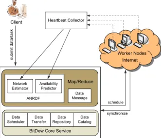
In this section, we briefly introduce the general overview of the proposed MapRe-duce system. The architecture is shown in Fig. 1. As is shown in this figure,
Client submit data and task, and Worker Nodes contribute their storage and
computing resources. The main components is described as follows,
– BitDew Core Service, the runtime environment of BitDew which contains Data Scheduler, Data Transfer, Data Repository, Data Catalog service;
Internet Client s u b m it d a ta /t a s k Heartbeat Collector Worker Nodes
BitDew Core Service Data Scheduler Data Catalog Data Repository Data Transfer schedule synchronize Map/Reduce Network Estimator Availability Predictor ANRDF Data Message
Fig. 1. Architecture of the proposed MapReduce system.
– Heartbeat Collector, collects periodical heartbeat signals from Worker Nodes; – Data Message, manages all the messages during the MapReduce
computa-tion;
– ANRDF, the availability and network-aware resource discovery framework,
including Network Estimator which estimates node distance using the land-mark and binning scheme, and Availability Predictor which predicts node availability using the Naive Bayes Classifier. This framework suggests prop-er nodes for scheduling.
Compared with our previous work BitDew-MapReduce [19], the proposed MapReduce system in this paper exploits two techniques, availability predic-tion and network distance estimapredic-tion, to overcome the volatility and low-speed network bandwidth between wide-area volunteer nodes.
3.2 Availability Prediction Based on Bayesian Model
Availability traces of parallel and distributed systems can be used to facilitate the design, validation, and comparison of fault-tolerant models and algorithms, such as the SETI@home traces2. It is a popular traces which can be used to
simulate a discrete event-driven volunteer computing system. Usually, the format of availability traces is {tstart, tend, state}. In detail, if the value of state is 1,
it means that the node is online between the time tstart and tend, while if the state equals 0, it means that the node is offline.
2
SETI@home is a global scientific experiment that uses Internet-connected computers in the Search for Extraterrestrial Intelligence. SETI@home traces can be downloaded from Failure Trace Archive (FTA), http://fta.scem.uws.edu.au/.
Our prediction method is measurement-based, that is, given a set of availabil-ity traces called training data, we create a predictive model of availabilavailabil-ity that is tested for accuracy with the subsequent (i.e., more recent) test data. For the sake of simplicity we refrain from periodic model updates. We use two windows (training window and test window), and move these two windows in order to get a lot of data (training data and test data).
Each sample in the training and test data corresponds to one hour and so it can be represented as a binary (01) string. Assuming that a prediction is computed at time T (i.e. it uses any data up to time T but not beyond it), we attempt to predict the complete availability versus (complete or partial) non-availability for the whole prediction interval [T, T + p]. The value of p is designated as the prediction interval length (pil) and takes values in whole hours (i.e. 1,2,...).
We compute for each node a predictive model implemented as a Naive Bayes Classifier, a classic supervised learning classifier used in data mining. A classifica-tion algorithm is usually the most suitable model type if inputs and outputs are discrete and allows the incorporation of multiple inputs and arbitrary features, i.e., functions of data which expose better its information content.
Features of training data We denote the availability (01 string) in the training
window as e = (e1, e2,· · · , en)T, where n is the number of the samples in the
training window, also known as training interval length (til). As an example, if the length of the training interval is in hour-scale, the training interval of 30 days is n = 720. Through the analysis of availability traces, we extract 6 candidate features to be used in Bayesian model, each of which can partially reflect recent availability fluctuation. The elements in the vector are organized from the oldest one to the most recent one. For example, en indicates the newest sample that is
closest to the current moment. We summarize the 6 features as follows.
– Average Node Availability (aveAva): It is the average node availability
in the training data.
– Average Consecutive Availability (aveAvaRun): It is the average length
of a consecutive availability run.
– Average Consecutive Non-availability (aveNAvaRun): It is the average
length of a consecutive non-availability run.
– Average Switch Times (aveSwitch): It is the average number of changes
of the availability status per week.
– Recent Availability (recAvak): It is the average availability in recent k
days (k=1, 2, 3, 4, 5), which is calculated by recent k days’ “history bits” (24, 48, 72, 96, 120 bits in total, respectively).
– Compressed Length (zipLen): It is the length of the training data
com-pressed by the Lempel-Ziv-Welch (LZW) algorithm.
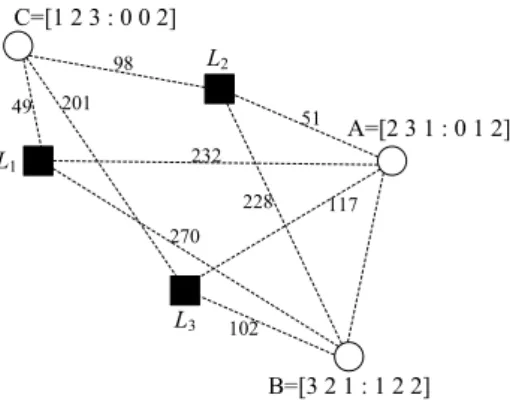
3.3 Network Distance Estimation Based on Binning Scheme
The classic binning scheme proposed by Ratnasamy et al. is adopted to obtain the topological information for network distance estimation in our proposed
ANRDF [16]. In the binning scheme, nodes partition themselves into bins such that nodes that fall within a given bin are relatively close to one another in terms of network latency. This scheme requires a set of well-known landmark machines spread across the Internet. An application node measures its distance, i.e. round-trip time (RTT), to this set of well known landmarks and independently selects a particular bin based on these measurements.
The form of “distributed binning” of nodes is achieved based on their relative distances, i.e. latencies from this set of landmarks. A node measures its RTT to each of these landmarks and orders the landmarks in order of increasing RTT. More precisely, if L = {l0, l1, ..., lm−1} is the set of m landmarks, then
a node A creates an ordering La on L, such that i appears before j in La if rtt(a, li) < rtt(a, lj) or rtt(a, li) = rtt(a, lj) and li < lj. Thus, based on its
delay measurements to the different landmarks, every node has an associated ordering of landmarks. This ordering represents the “bin” the node belongs to. The rationale behind this scheme is that topologically close nodes are likely to have the same ordering and hence will belong to the same bin.
L2 L1 L3 51 232 117 98 49 201 A=[2 3 1 : 0 1 2] B=[3 2 1 : 1 2 2] C=[1 2 3 : 0 0 2] 228 270 102
Fig. 2. Distributed binning.
We can however do better than just using the ordering to define a bin. A nodes RTT measurements to each landmark offers two kinds of information: the first is the relative distance of the different landmarks from the given node and the second is the absolute value of these distances. The ordering described above only makes uses of the relative distances of the landmarks from a node. The absolute values of the RTT measurements are indicated as follows: we divide the range of possible latency values into a number of levels. For example, we might divide the range of possible latency values into 3 levels; level 0 for latencies in the range [0,100]ms, level 1 for latencies between [100,200]ms and level 2 for latencies greater than 200ms. We then augment the landmark ordering of a node with a level vector; one level number corresponding to each landmark in the ordering. To illustrate, consider node A in Fig. 2. Its distance to landmarks
landmarks is l2 l3 l1. Using the 3 levels defined above, node A’s level vector
corresponding to its ordering of landmarks is “0 1 2”. Thus, node A’s bin is a vector [Va: Vb] = [2 3 1 : 0 1 2], as is shown in Fig. 2.
4
Map/Reduce Algorithm and Implementation
Our previous work introduced the architecture, runtime, and performance e-valuation of BitDew-MapReduce [19]. In this section, we first give a detailed description of the regular BitDew-MapReduce, then present how to improve it through availability prediction and network distance estimation. When the user aims to achieve a MapReduce application, the master splits all files into chunks, registers and uploads all chunks to the BitDew services, which will be scheduled and distributed to a set of workers as input data for Map task. When a worker receives data from the BitDew service node, a data scheduled event is raised. At this time it determines whether the received data is treated as Map or Reduce input, and then the appropriate Map or Reduce function is called.
As mentioned previously, BitDew allows the programmer to develop data-driven applications. That is, components of the system react when Data are scheduled or deleted. Data are created by nodes either as simple communication messages (without “payload”) or associated with a file. In the later case, the respective file can be sent to the BitDew data repository service and scheduled as input data for computational tasks. The way the Data is scheduled depends on the Attribute associated to it. An attribute contains several (key, value) pairs which could influence how the BitDew scheduler will schedule the Data.
The BitDew API provides a schedule(Data, Attribute) function by which, a client requires a particular behavior for Data, according to the associated
Attribute.
Algorithm 1 Data Creation
Require: Let F ={f1, . . . fn} be the set of input files
1. {on the Master node}
2. Create a DC, a DataCollection based on F 3. Schedule data DC with attribute M apInputAttr
The initial MapReduce input files are handled by the Master (see Algorithm 1). Input files can be provided either as the content of a directory or as a single large file with a file chunk size Sc. In the second case, the Master splits the large
file into a set of file chunks, which can be treated as regular input files. We denote
F = {f1, . . . fn} the set of input files. From the input files, the Master node
creates a DataCollection DC = {d1, . . . , dn}, and the input files are uploaded
to BitDew. Then, the master creates Attribute M apInputAttr with replica=1 and distrib=-1 flag values, this means that each input file is one input data for
the Map task. Each di is scheduled according to the M apInputAttr attribute.
The node where di is scheduled will get the content associated to the respective Data, that is fi as input data for a Map task.
The Algorithm 2 presents the Map phase. To initiate a MapReduce dis-tributed computation, the Master node first creates a data M apT oken, with an attribute whose affinity is set to the DataCollection DC. This way, M apT oken will be scheduled to all the workers. Once the token is received by a worker, the Map function is called repeatedly to process each chunks received by the worker, creating a local list(k, v).
Algorithm 2 Execution of Map tasks
Require: Let M ap be the Map function to execute
Require: Let M be the number of Mappers and m a single mapper
Require: Let dm={d1,m, . . . dk,m} be the set of map input data received by worker
m
1. {on the Master node}
2. Create a single data M apT oken with affinity set to DC 3.
4. {on the Worker node}
5. if M apT oken is scheduled then 6. for all data dj,m∈ dmdo
7. execute M ap(dj,m)
8. create listj,m(k, v)
9. end for
10. end if
After finishing all the Map tasks, the worker splits its local listm(k, v)
in-to r intermediate output result files ifm,r according to the partition function,
and R, the number of reducers (see Algorithm 3). For each intermediate files
ifm,r, a reduce input data irm,r is created. How to transmit irm,r to their
cor-responding reducer? This is partly implemented by the master, which creates R specific data called ReduceT okenr, and schedules this data with the attribute ReduceT okenAttr. If one worker receives the token, it is selected to be a reducer.
As we assume that there are less reducers than workers, the ReduceT okenAttr has distrib=1 flag value which ensures a fair distribution of the workload be-tween reducers. Finally, the Shuffle phase is simply implemented by scheduling the portioned intermediate data with an attribute whose affinity tag is equal to the corresponding ReduceT oken.
Algorithm 4 presents the Reduce phase. When a reducer, that is a worker which has the ReduceT oken, starts to receive intermediate results, it calls the Reduce function on the (k, list(v)). When all the intermediate files have been received, all the values have been processed for a specific key. If the user wishes, he can get all the results back to the master and eventually combine them. To proceed to this last step, the worker creates an M asterT oken data, which is
Algorithm 3 Shuffling intermediate results
Require: Let M be the number of Mappers and m a single worker Require: Let R be the number of Reducers
Require: Let listm(k, v) be the set of (key, value) pairs of intermediate results on worker m
1. {on the Master node}
2. for all r∈ [1, . . . , R] do
3. Create Attribute ReduceAttrr with distrib = 1
4. Create data ReduceT okenr
5. schedule data ReduceT okenrwith attribute ReduceT okenAttr
6. end for 7.
8. {on the Worker node}
9. split listm(k, v) in{ifm,1, . . . , ifm,r} intermediate files
10. for all file ifm,r do
11. create reduce input data irm,r and upload ifm,r
12. schedule data irm,r with af f inity = ReduceT okenr
13. end for
Algorithm 4 Execution of Reduce tasks
Require: Let Reduce be the Map function to execute
Require: Let R be the number of Mappers and r a single worker
Require: Let irr = {ir1,r, . . . irm,r} be the set of intermediate results received by
reducer r
1. {on the Master node}
2. Create a single data M asterT oken 3. pinAndSchedule(M asterT oken) 4.
5. {on the Worker node}
6. if irm,r is scheduled then
7. execute Reduce(irm,r)
8. if all irr have been processed then
9. create or with af f inity = M asterT oken
10. end if
11. end if 12.
13. {on the Master node}
14. if all orhave been received then
15. Combine or into a single result
pinnedAndScheduled. This operation means that the M asterT oken is known
from the BitDew scheduler but will not be sent to any nodes in the system. Instead, M asterT oken is pinned on the Master node, which allows the result of the Reduce tasks, scheduled with a tag affinity set to M asterT oken, to be sent to the Master.
We detail now how to integrate availability prediction and network distance estimation into our previous BitDew-MapReduce framework.
– Measurement : Each worker measures the RTT to each landmarks, and in
the initiation of worker, it sends back the RTT value to the master. Work-ers periodically synchronizes with the master, in our prototype the typical synchronization interval is 10s, while it is configurable. A timeout-based approach is adopted by the worker to detect worker failure, and failure in-formation is written to a log file which is used for generating availability traces.
– Availability ranking: The availability traces are stored in the master, and the
master manages a ranking list. The list is updated when a synchronization is arrived. Workers are sorted by the predicted availability in the future pre-diction interval length, and we also considered the stableness of each worker by average switch times (aveSwitch) and recent availability (recAvak).
– How to use availability information for scheduling? The worker with low
availability and low stableness will stop accepting data, which makes sure that the master distributes input data and ReduceT oken to more stable nodes.
– Network proximity: The master manages all the RTT values and “bins”, each
node (no matter the worker or the landmark) is assigned with a bin vector. Suppose that there are two nodes n1and n2with two vectors V1= [V1a : V1b]
and V2= [V2a : V2b], respectively. The proximity degree (or we say distance)
of n1and n2 can be calculated by the Euclidean distance of vector V1a and
V2a. While if V1a equals to V2a, we calculate using the vector V1b and V2b
instead. If the proximity degree is smaller than a given threshold, they are locates in the same “bin”.
– How to use network information for scheduling? In order to avoid the load
balancing problem, when a DataCollection is created and needed to be dis-tributed to workers, a landmark is selected by random, and it also means that this landmark will “serve” this MapReduce job. The bin vector of this landmark is broadcasted to all the workers, and the workers that locate in the same bin with this landmark could accept input data. All the ReduceT oken are also distributed to R workers that locate in the same bin. In our frame-work, the network feature is stronger than availability feature. Therefore, the intermediate results will be transferred to a closer node due to that both the mapper and the reducer locate in the same bin.
5
Performance Evaluation
We implemented the prototype system using BitDew middleware with Java. We conducted a simulation-based evaluation to test the performance of new
MapRe-duce framework. First, the effectiveness of Naive Bayes Classifier is validated. Since that the landmark-based network proximity has been studied in [16], we focus on the simulation of MapReduce jobs running in a large-scale dynamic en-vironment, considering availability prediction and network distance estimation. Simulations are performed on an Intel Xeon E5-1650 server.
5.1 Availability Prediction
Availability traces We evaluate our predictive methods using real availability
traces gathered from the SETI@home project. In our simulation, we used 60 days’ data from real SETI@home availability traces. The SETI@home traces contain the node availability information (online or offline) of dynamic large-scale nodes over Internet (around 110K nodes for the full traces) [9]. We generate a trace subset for our simulations by randomly selecting 1,000 nodes from the full SETI@home traces, then we perform a statistic analysis on those selected nodes, and the characteristics are presented as follows: up to around 350 nodes (approximately 35%) are online simultaneously; and around 50% of nodes whose availability are less than 0.7.
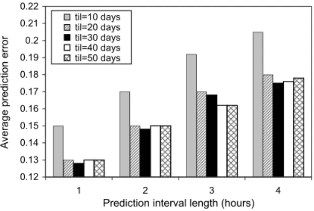
The impact of training interval length and prediction interval length
We studied the dependence of the prediction error on the training interval length (til) and the prediction interval length (pil) value for the randomly selected hosts, using the Naive Bayes Classifier proposed above. Fig. 3 shows average prediction error, depending on the pil=1, 2, 3, 4, while training days=10, 20, 30, 40, 50. While the error decreases significantly if the amount of training data increases from 10 to 20 days, further improvements are marginal. The higher pil value makes higher prediction error. This is a consequence of increased uncertainty over longer prediction periods and the “asymmetric” definition of availability in the prediction interval (a short and likely random intermittent unavailability makes the whole interval unavailable). We have therefore used 30 days as the amount of training data for the remainder of this paper, and 4 hours as the prediction interval length.
Algorithms for comparison In addition to our Naive Bayes Classifier (N-BC)
method, we also implemented five other prediction methods. Some of them have been shown to be effective in discrete sequence prediction. Under our formulated prediction model, we make them uniformly aim to predict availability of the future interval, based on the training data.
– Last-State Based Method (LS): The last recorded value in the training data
will be used as the predicted value for the future period.
– Simple Moving Average Method (SMA): The mean value of the training
data will serve as the predicted value.
– Linear Weighted Moving Average Method (WMA): The linear weighted
0.12 0.13 0.14 0.15 0.16 0.17 0.18 0.19 0.2 0.21 0.22 1 2 3 4
Prediction interval length (hours)
A v e ra g e p re d ic ti o n e rr o r til=10 days til=20 days til=30 days til=40 days til=50 days
Fig. 3. Prediction error depending on til and pil.
mean value for the future. Rather than the mean value, the weighted mean value weights the recent value more heavily than older ones.
Fwrt(e) = n ∑ i=1 iei/ n ∑ i=1 i (1)
– Exponential Moving Average Method (EMA): This predicted value (denoted S(t) at time t) is calculated based on the Equation (2), where e1 is the last
value and α is tuned empirically to optimize accuracy.
S(t) = α· e1+ (1− α) · S(t − 1) (2)
– Prior Probability Based method (PriorPr): This method uses the value with
highest prior probability as the prediction for the future mean value, regard-less of the evidence window.
The training period is used to fit the models. The test period is used to validate the prediction effect of different methods. In our evaluation, the size of training data is 30 days (the length of the 01 training string is 720). The key parameters used for evaluation are as follows: in the EMA method, the value of
α is 0.90.
In terms of evaluating prediction accuracy, we use two metrics. First, we measure the mean squared error (MSE) between the predicted values and the true values in the prediction interval. Second, we measure success rate, which is defined as the ratio of the number of accurate predictions to total number of predictions. In general, the higher the success rate, the better, and the lower the MSE.
Fig. 4(a) and 4(b) shows the cumulative distribution function (CDF) of the success rate and MSE for different prediction methods, respectively. For the success rate comparison, the curve which is more closer to the bottom-right corner is better, while for the MSE comparison, the curve which is near the top-left corner is better. Therefore, it is clear that N-BC’s prediction effect is better
0 0.2 0.4 0.6 0.8 1 0 0.2 0.4 0.6 0.8 1 Success Rate CDF N−BC PriorPr LS SMA WMA EMA
(a) CDF of success rate
0 20 40 60 80 0 0.2 0.4 0.6 0.8 1 MSE CDF N−BC PriorPr LS SMA WMA EMA (b) CDF of MSE
Fig. 4. Prediction accuracy comparison using different methods (training days = 30)
than all the other methods. From Fig. 4(a), it is observed that SMA (Simple Moving Average Method) performs poorly, while LS (Last-State Based Method) performs poorly in Fig. 4(b). The reason why Bayesian prediction outperforms other methods is its features, which capture more complex dynamics, which have not been made by LS and SMA methods.
5.2 Simulation of the Proposed MapReduce Framework
In order to integrate the network prediction approach, BRITE is used as a topolo-gy generator, which can generate wide-area network topolotopolo-gy according to user-predefined parameters [14]. We create a wide-area network composed of 1015 nodes. Among them, 14 nodes are supposed to be landmarks, and 1 node serves as the server. For other 1000 nodes, we assign each node an ID, and also assign each node a trace from the subset of SETI@home that we selected before.
In order to evaluate how well the proposed MapReduce performs over the Internet environment, we borrowed some ideas from GridSim [2], a famous Grid simulation toolkit. We build a discrete event based simulator, which loads avail-ability traces of each node, and manages an event queue. It reads a BRITE file and generates a topological network from it. Information of this network is used to simulate latency and data transfer time estimation. We define the CPU capability for each node. We also define a model of MapReduce job, and seven parameters are configured to describe a MapReduce job, including the size of input data, the size of DFS chunk, the size of intermediate file (corresponding to Map task result of each chunk), the size of final output file, the number of Mappers, the number of Reducers, and the option of fast application pattern or slow application pattern. The fast pattern means that Mapper/Reducer time is long, while the slow pattern has short Mapper/Reducer time. We also considered the following four kinds of MapReduce jobs in the simulation:
2) Model B: fast application, small intermediate file size; 3) Model C: slow application, large intermediate file size; 4) Model D: slow application, small intermediate file size.
We considered the following four scenarios when scheduling MapReduce jobs over the Internet:
1) Scenario I: without any strategies;
2) Scenario II: with availability prediction only; 3) Scenario III: with network estimation only;
4) Scenario IV: with availability prediction and network estimation together. The main model specific parameters in BRITE topology generator are as follows: node placement is random; bandwidth distribution is exponential dis-tribution (the value of M axBW is 8192, and the value of M inBW is 30). For a MapReduce job, the input data size is set to a random value between 50GB and 200GB, and DFS chunk size is 64MB, and intermediate file size for a Mapper is set to 150MB (corresponding to large) and 50MB (corresponding to small). For fast jobs, data processing speed for a Mapper or Reducer is 10MB/GHz; while the value is 1MB/GHz for slow jobs. The CPU capacity of node is a random value between 1GHz and 3GHz. We start the simulator, submit 100 MapReduce jobs, and then estimate the job completion time.
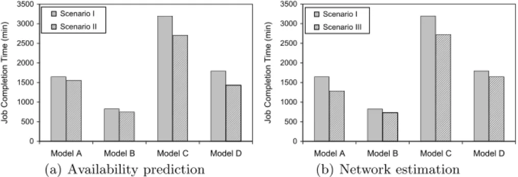
Availability prediction only First, we compared Scenario I with Scenario
II, to validate the improvement of MapReduce job completion time, when the availability prediction method is used. As we can see in Fig. 5(a), Scenarios II outperforms Scenarios I, and job completion time is decreased when using availability prediction. With the availability prediction, task failure and task re-scheduling ratio has been decreased, especially for the Model C and Model D. For the slow MapReduce jobs, Map or Reduce task have higher possibility to be failed and needed to re-scheduled. From this figure, it is also indicated that there is also only little performance difference for Model A and Model B.
0 500 1000 1500 2000 2500 3000 3500
Model A Model B Model C Model D
J o b C o m p le ti o n T im e ( m in ) Scenario I Scenario II
(a) Availability prediction
0 500 1000 1500 2000 2500 3000 3500
Model A Model B Model C Model D
J o b C o m p le ti o n T im e ( m in
) Scenario I Scenario III
(b) Network estimation
Network estimation only Because network distance has impact on data
trans-fer time, we compared Scenario I with Scenario III in this evaluation, and the result is presented by Fig. 5(b). Intermediate file size and the number of land-mark are two important factors for MapReduce job completion time. If the landmark-based network estimation is not used, the server doesn’t consider any information or attributes of nodes and all nodes are treated equally, which may cause the problem that transferring intermediate data to a far desktop PCs. For Model A and Model C, it takes more time to transfer large intermediate file, and the job completion time is decreased by 21.93% and 14.68% respectively, when the network estimation method is used in Scenario III.
We also evaluated job completion time when configuring different number of landmark, and we adopted the Model A for evaluation. The number of landmark is increased from 4 to 14, and the step size is 2. As the increase of landmark num-ber, MapReduce job completion time is also decreased from 1522min, 1411min, 1332min, 1288min, 1278min to 1262min, due to that with larger number of landmark, the network estimation can be more precise. While with too many landmarks, the algorithm of ‘binning’ is more complex. Usually, 8-12 landmarks should suffice for the current scale of the Internet [16]. Therefore, we used 10 landmarks in our previous evaluations.
Comparison of different strategies We also conducted the comparison of
different strategies, as we mentioned before, Scenario I, II, III and IV. For the MapReduce jobs, we evaluated all the four patterns. The comparison result is presented in Fig. 6, and Scenario IV outperforms all other scenarios. Scenario IV improves the MapReduce system and decreases the overall job response time, through combining two scheduling strategies: availability-aware and network-aware scheduling. Compared with Scenario I, the performance improvement of Scenario IV is 27.15% for Model A, 24.09% for Model B, 18.43% for Model C, and 23.44% for Model D, respectively.
0 400 800 1200 1600 2000 2400 2800 3200 3600 4000
Model A Model B Model C Model D
J o b C o m p le ti o n T im e ( m in ) Scenario I Scenario II Scenario III Scenario IV
6
Conclusion
MapReduce offers an ease-of-use programming paradigm for processing large data sets, making it an attractive model for distributed volunteer computing systems. In our previous work, we have designed a MapReduce framework called BitDew-MapReduce for desktop grid and volunteer computing environment, that allows nonexpert users to run data-intensive MapReduce jobs on top of volunteer resources over the Internet. However, network distance and resource availabili-ty have great impact on MapReduce applications running over the Internet. To address this, we proposed an availability and network-aware MapReduce frame-work on Internet. It outperforms current MapReduce frameframe-work on Internet, thanks to Naive Bayes Classifier-based availability prediction and landmark-based network estimation. The performance evaluation results were obtained by simulations. In the simulation, the real SETI@home availability traces was used for validation, and BRITE topology generator was used to generate a low-speed, wide-area network. Results show that the Bayesian method achieves higher accu-racy compared with other prediction methods, and intermediate results could be transferred to a more closer nodes to perform Reduce tasks. With the resource availability prediction and network distance estimation method, the MapReduce job response time could be decreased conspicuously.
Acknowledgement This work is supported by the “100 Talents Project” of
Computer Network Information Center of Chinese Academy of Sciences under grant no. 1101002001, and the Natural Science Foundation of Hunan Province under grant no. 2015JJ3071, and Scientific Research Fund of Hunan Provincial Education Department under grant no. 12C0121, 11C0689 and 11C0535.
References
1. Anderson, D.P.: Boinc: A system for public-resource computing and storage. In: GRID. pp. 4–10. IEEE (2004)
2. Buyya, R., Murshed, M.: Gridsim: A toolkit for the modeling and simulation of distributed resource management and scheduling for grid computing. Concurrency and Computation: Practice and Experience 14(13), 1175–1220 (2002)
3. Costa, F., Silva, J.N., Veiga, L., Ferreira, P.: Large-scale volunteer computing over the internet. J. Internet Services and Applications 3(3), 329–346 (2012)
4. Costa, F., Silva, L.M., Fedak, G., Kelley, I.: Optimizing data distribution in desktop grid platforms. Parallel Processing Letters 18(3), 391–410 (2008)
5. Costa, F., Veiga, L., Ferreira, P.: Internet-scale support for map-reduce processing. J. Internet Services and Applications 4(1), 1–17 (2013)
6. Dean, J., Ghemawat, S.: Mapreduce: simplified data processing on large clusters. Commun. ACM 51(1), 107–113 (2008)
7. Fedak, G., He, H., Cappello, F.: Bitdew: A data management and distribution service with multi-protocol file transfer and metadata abstraction. J. Network and Computer Applications 32(5), 961–975 (2009)
8. Jin, H., Yang, X., Sun, X.H., Raicu, I.: Adapt: Availability-aware mapreduce data placement for non-dedicated distributed computing. In: ICDCS. pp. 516–525. IEEE (2012)
9. Kondo, D., Javadi, B., Iosup, A., Epema, D.H.J.: The failure trace archive: En-abling comparative analysis of failures in diverse distributed systems. In: CCGRID. pp. 398–407. IEEE (2010)
10. Lee, K., Figueiredo, R.J.O.: Mapreduce on opportunistic resources leveraging re-source availability. In: CloudCom. pp. 435–442. IEEE (2012)
11. Lin, H., Ma, X., chun Feng, W.: Reliable mapreduce computing on opportunistic resources. Cluster Computing 15(2), 145–161 (2012)
12. Lu, L., Jin, H., Shi, X., Fedak, G.: Assessing mapreduce for internet computing: A comparison of hadoop and bitdew-mapreduce. In: GRID. pp. 76–84. IEEE Com-puter Society (2012)
13. Marozzo, F., Talia, D., Trunfio, P.: P2p-mapreduce: Parallel data processing in dynamic cloud environments. J. Comput. Syst. Sci. 78(5), 1382–1402 (2012) 14. Medina, A., Lakhina, A., Matta, I., Byers, J.W.: Brite: An approach to universal
topology generation. In: MASCOTS. IEEE Computer Society (2001)
15. Moca, M., Silaghi, G.C., Fedak, G.: Distributed results checking for mapreduce in volunteer computing. In: IPDPS Workshops. pp. 1847–1854. IEEE (2011) 16. Ratnasamy, S., Handley, M., Karp, R.M., Shenker, S.: Topologically-aware overlay
construction and server selection. In: INFOCOM (2002)
17. Song, S., Keleher, P.J., Bhattacharjee, B., Sussman, A.: Decentralized, accurate, and low-cost network bandwidth prediction. In: INFOCOM. pp. 6–10. IEEE (2011) 18. Tang, B., He, H., Fedak, G.: Parallel data processing in dynamic hybrid computing
environment using mapreduce. In: ICA3PP (2014)
19. Tang, B., Moca, M., Chevalier, S., He, H., Fedak, G.: Towards mapreduce for desktop grid computing. In: 3PGCIC. pp. 193–200. IEEE Computer Society (2010) 20. Wei, B., Fedak, G., Cappello, F.: Towards efficient data distribution on computa-tional desktop grids with bittorrent. Future Generation Comp. Syst. 23(8), 983–989 (2007)
21. Zaharia, M., Konwinski, A., Joseph, A.D., Katz, R.H., Stoica, I.: Improving mapre-duce performance in heterogeneous environments. In: OSDI. pp. 29–42. USENIX Association (2008)