Calculation of the second order mean force on a ship in oblique seas.

ON A SHIP IN OBLIQUE SEAS

by

PAUL ROSS ERB

S.B., Massachusetts Institute of Technology (1976)

SUBMITTED IN PARTIAL FULFILLMENT OF THE REQUIREMENTS FOR THE DEGREES OF

MASTER OF SCIENCE

IN NAVAL ARCHITECTURE AND MARINE ENGINEERING AND

MASTER OF SCIENCE IN MECHANICAL ENGINEERING

at the

MASSACHUSETTS INSTITUTE OF TECHNOLOGY

June, 1977

Signature of Author .

Departmentsof Ocean Engineering

,May 12, 1977

Certified by .

/ Thesis Supervisor Department of Ocean Engineering

Certified by ...

Department Reader Department of Mechanical Engineering

Accepted by . ...

Chairman, Departmentl Committee on Graduate Students

r ~ives

CALCULATION OF THE SECOND ORDER MEAN FORCE

ON A SHIP IN OBLIQUE SEAS

by

PAUL ROSS ERB

Submitted to the Department of Ocean Engineering and the Department of Mechanical Engineering on May 12, 1977 in partial fulfillment of the requirements for the Degree of

Master of Science in Naval Architecture and Marine Engineering and the Degree of Master of Science in Mechanical Engineering.

ABSTRACT

A design tool is developed for use by engineers for the calculation of the mean added resistance or drift force on an elongated body such as a ship in a seaway. Only

forces arising from wave-ship motion interaction or wave reflection are considered and developed in a form suitable for a computer program. This procedure allows computation of the mean second order force from first order quantities already known in strip theory of ship motions. Regular wave computer results generated by the MIT 5-D motions program for the Mariner cargo vessel are presented and compared with experiment, including a set of new beam seas experiments. Comparison is also made with published re-sults from two other programs. The extension of the regular wave theory to an irregular long-crested seaway and then to a short-crested seaway is outlined. Finally, six representative sea spectra are used in a brief design analysis for the Mariner at service speed.

Thesis Supervisor: Chryssostomos Chryssostomidis

ACKNOWLEDGEMENTS

The author wishes to extend his sincere appreciation for the help and guidance given to him by his advisor, Professor C. Chryssostomidis, not just on this thesis, but throughout his undergraduate and graduate years at M.I.T.

This work would have been very difficult to complete if not for the efforts of several individuals. The experi-mental work was done with the help of Ysabel Meija. Pro-fessors Owen Oakley and Martin Abkowitz generously offered advice and opinions at various stages. Fraternity brothers, Stephen K.Gourley and David B. S. Smith gave invaluable

assistance by producing many of the final graphs and figures. Barbara Belt read portions of the draft and

offered valuable suggestions. Special thanks are also

extended to Elaine Govoni, who prepared the final manu-script.

All computations were performed at the M.I.T. Information Processing Center with a grant from the National Science Foundation. In closing, the author wishes to express his gratitude to the Society of Naval

Architects and Marine Engineers for their generous

graduate scholarship and to his family for their unfailing support.

TABLE OF CONTENTS

Title Page . . . . . . . . . . . . . .

Abstract .... . . .... ...

Acknowledgements . . . . . . . . . . .

Table of Contents . . . . . . . . . .

List of Figures and Tables . . . . . .

List of Symbols . . . . . . . . . . .

CHAPTER I Introduction . . . . . .

CHAPTER II Historical Background . .

CHAPTER III Theoretical Development .

CHAPTER IV Verification of Theory .

CHAPTER V CHAPTER VI

References Appendices:

A. Comparison with Experimental Results. 64 B. Comparison with Other Theoretical

Results . . . . . . . . . . . . . . . 75

Design Analysis. . ... 93

Condlusion and Recommendations. . . . . . 110

. . . .. 114

A. Changes to M.I.T. 5-D Seakeeping Program User's Manual . . . . . . . . 117

B. Sample Output . ... 119

C. Subroutines Modified . . . . . . . . 128

D. Listing of Mariner Example Data . . . 169

. . . 12

. . . 16

. . . 24

S . .

60

LIST OF FIGURES AND TABLES

Figures

No. Title Page

1 Coordinate System . ... . 25

2 Mariner Added Resistance Components

(Terms in Eq. (86)) . . . 62

3 Added Resistance/Head Waves . . . . . . . . 66

4 Mariner Model; U=0; A=900 .. . ... . 71

5 Mariner Model; U=0; 3=1050 . . . . . . .. 72

6 Mariner Model; U=0; 3=750 . ... 73

7 Mariner - Added Resistance Head Waves

(p=1800 _{) Various Speeds . ... 77}

8 Mariner - Added Resistance

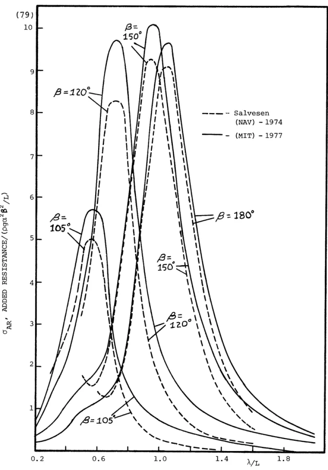
(Speed - 15 knots) Various Headings . . .. 79

9 Mariner - Added Resistance

(Speed - 15 knots) Various Headings . . . . 80

10 Mariner - Drift Force

(B=1200) Various Speeds ... 82

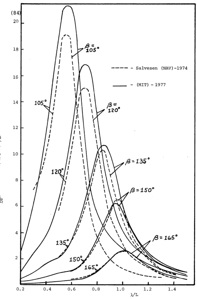
11 Mariner - Drift Force

(Speed - 15 knots) Various Headings . ... 84

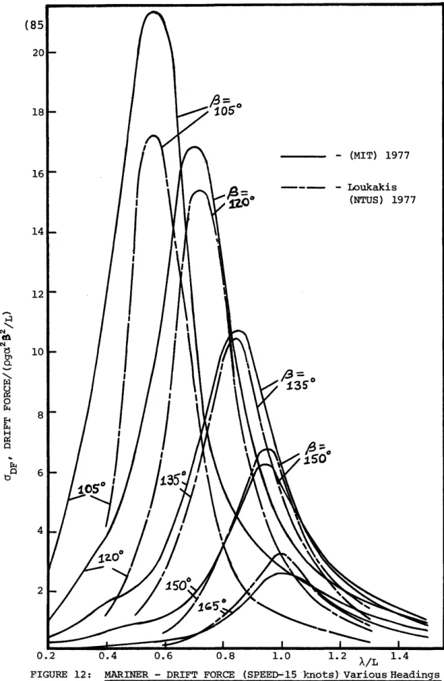
12 Mariner - Drift Force

(Speed - 15 knots) Various Headings . . . . 85

13 Mariner - Negative Added Resistance

(Speed - 15 knots) Various Headings . . . . 87

14 Mariner - Drift Force

(Speed - 15 knots) Various Headings . . . . 88

15 Sea Spectra .. ... . .. . . . . . . 98

16 Mariner Irregular Seas Results .. ... . 100

Figures No.

(Continued Title

17 Mariner Irregular Seas Results

(Mean Drift Force; Pierson-Moskowitz) . .

18 Mariner Irregular Seas Results

(Mean Added Resistance; Bretschneider) 19 Mariner Irregular Seas Results

(Mean Drift Force; Bretschneider)

Tables

Added Resistance/Drift Force in Pou:

for Various Sea States . . . . . .

. . .

0.

LIST OF SYMBOLS a(x) or ajk(X) AX_x Ajk b b(x) or bjk(x) b* (x) B Bjk CA Cjk

d

f (x)

- Sectional added mass coefficient - Sectional area

- Added mass matrix of the ship - Sectional beam

- Sectional damping coefficient

- Gerritsma and Beukelman sectional

quantity (3a)

- Ship beam

- Damping matrix of the ship - After cross-section

- Hydrostatic restoring force matrix of the ship

- Sectional draft

- Radiated energy from ship

- Energy spectrum of the sea based on full

wave amplitude

- Functional relation

- Sectional Froude-Kriloff force

- Mean second order force in long-crested

irregular seas

- Mean second order force in short-crested

irregular seas

- Complex exciting force vector

FjI - Froude-Kriloff portion of exciting force

F - Unsteady hydrodynamic force vector

- Mean value of F

C4- Magnitude of 3

'D - Component of I related to the

diffrac-tion potential

jx - Added resistance component of second

order force

0 y - Drift force component of second order

force

j·I - Component of c related to the

Froude-Kriloff excitation

C4D - Component otf 'analogous to the

dif-fraction excitation

g - Gravitational acceleration

Gj - Added mass and damping part of H.

hD(x) - Sectional quantity, integrand of53D (81)

hj(x) - Sectional diffraction force

'h1/ 3 - Significant wave height

hj(x) - Sectional quantity, integrand of*.D (78d)

H. - Total hydrodynamic force vector

i - /-1

I_{D - Integral used to develop'D expressicn}

(82)

Ijk - Moment or product of inertia

j - Subscript (1...6; surge, sway, heave,

roll, pitch, yaw)

similar 1-l -i

K - Wave number

L - Ship length (L.B.P.)

mk - Related to ship normal, nk

Mjk - Mass matrix of the ship

n_k - Ship hull normal (generalized)

Nj - Two-dimensional normal

p - Pressure in fluid

Q - Represents either A or B

S - Ship surface

SF - Free surface

So - Control surface at infinity

tjk _{- Sectional integrand of Tjk}

Tjk _{- Complex quantity giving the Ajk and Bjk}

elements

U - Forward velocity of ship

V - Volume within S, SF, So

Vza(X) - Relative sectional velocity

x - Longitudinal axis of the ship

x_b - Distance from center of gravity to

center of buoyancy

y - Transverse axis of the ship

z - Vertical axis of the ship

Zc - Coordinate of the center of gravity

a- Wave amplitude (1/2 height)

Ck - Phase angle between motion and exci-tation

- Free surface position

Sk

p* - Corrected free surface velocity

6 - Principal wind direction for

short-crested seas

X - Wave length

- Difference between heading angle ý and

wind direction 8

p - Water density

- Sectional area coefficient (Ax/bd)

•B - Full body potential amplitude

PD - Diffraction potential amplitude

4_{DC - Non-zero mean higher order potential}

ýI - Incident wave potential amplitude

ck - Motion potential amplitude

•ko - Speed independent motion potential

kU - Speed dependent motion potential

ýS - Steady state potential

ýT - Time dependent potential amplitude

- Overall velocity potential

•B - Full body potential

- Full incident wave potential

§+(W) - Sea spectrum based on half the wave amplitude

Tk - Two-dimensional (sectional potential

W _{- Encounter frequency (rad/sec)}

W_o - Incident wave frequency (rad/sec)

Wp - Spectral peak frequency (rad/sec)

I. INTRODUCTION

The forces that act on a ship in a seaway vary widely both in their nature and their relative importance. In general, they represent random processes which can only be quantified meaningfully through statistical analysis. Be-cause of this complexity, naval architects have traditionally been forced to make many design decisions by combining

judgement and experience with the results of comparatively simple, idealized analysis or experiments. One example of this process is the use of the ship-beam analogy and the quasistatic trochoidal wave profile for ship structural design. Another illustration can be found in the procedure used to determine ship power requirements. Common practice has been to obtain the results of calm water resistance and

self-propulsion model tests, then, to account for the actual operating conditions by applyinga power increase of fifteen to thirty percent. This service margin must be appropriate

if the ship is to fulfill her owner's requirements consis-tently, efficiently, and economically in the real ocean environment.

Recently, great progress has been made in the effort to include rigorously in the design process some of the factors that influence a ship at sea. The first order

strip theory of ship motions, due originally to

Korvin-Kroukovsky and Jacobs [1 31 , has been extended to the point

where motions can be calculated acceptably for a wide variety of ship types, sea states, and heading angles. This makes possible the calculation of dynamic loadings imposed on the

ship by a seaway (Salvesen, et. al [2 7 , and others).

Statis-tical methods developed for systems subject to random excitation now provide useful probabilistic statements concerning significant design events (e.g., the chance of slamming or the highest likely bending moment).

Due in part to these advances, the problem of environ-mental influence on ship power requirements and the related problem of the sideways drift of a ship in a seaway can now be much more fully addressed. The forces involved can be traced to a wide variety of sources, for example:

1. The motions of the ship interact with the ocean

waves to produce a net drift or added resistance. 2. The ocean waves reflect off the ship hull causing

a net force.

3. Wind present at sea acts on the superstructure to cause a drift force and/or an extra resistance. 4. Marine fouling causes an increase in resistance due

to surface roughness.

5. Involved interactions will also be present (e.g., the propeller may operate less efficiently due to

the ship motion, rudder motions necessary for coursekeeping might cause induced drag and side force, or the side slip of the whole vessel might similarly cause drag).

The complexity of the problem outlined still precludes complete analysis. However, it can be appreciated that even a partial solution, which reduces the significance of purely judgemental factors like the service margin, will greatly

increase the confidence and capability of the navalarchitect. This is particularly true for design decisions that break

new ground for the profession such as powering for ultra-large tankers, vessels on new trade routes, or even dynami-cally positioned drilling ships.

In order to developa useful, flexible design tool of this nature, the following report addresses the portion of the drift force/added resistance problem included in the

first two points above, namely theship motion-wave inter-action and the reflection. From this point, 'drift force' and 'added resistance' refer strictly to mean forces averaged during one wave period of encounter and caused by wave-ship

hull interaction. 'Added resistance' will be the term for

the mean force component parallel to the longitudinal, ship

axis, positive toward the stern. 'Drift force' will signify

the mean force component perpendicular to the longitudinal ship axis, positive when directed toward the same

half-plane as the wave propagation.

To place the method to be presented in a historical perspective, the paper begins with a discussion of past

analytical efforts on the problem. Then a brief description of first order strip theory of ship motions ispresented, and the method of calculation of second order mean wave

force developed by Salvesen [2 8 ] is detailed. As will be

seen, it is the mean second order wave force which is the drift force/added resistance referred to above. After an investigation of the characteristics of the final Salvesen formulation, an outline of past experimental work done on the problem is given, and an experimental effort devised to test certain areas of applicability is described. Following presentation of the experimental results, some numerical predictions for regular waves are compared with the results

S28e [162

shown by Salvesen and Loukakis [1 6 ]. The theoretical

basis for a probabalistic extension of the regular wave theory to irregular ocean conditions is described, and a brief design analysis for several sea states is given. Finally, some general conclusions and recommendations are offered. The appendices contain documentation for the computer program developed in the analysis.

II. HISTORICAL BACKGROUND

Kreitner was one of the earliest researchers (1939)

to investigate the problem of wave forces on a ship hull. He concluded that the force was caused primarily by the reflection of the incident waves from the hull. However, the real pioneer in the second order force problem was

Havelock '9 who proposed a theory in 1942 for a ship with

no forward speed in regular head seas that was allowed to pitch and heave. He found that Kreitner's reflection force was unrealistic for a pitching and heaving ship in waves of

reasonable length. Instead it became clear that the phase

difference between the ship motion and wave excitation was the primary source of added resistance. Following this

line of thought, Havelock proposed the following:

-

2-

where F I is the exciting force or moment due to the wave

(assuming that the ship does not affect the wave flow field); this force (moment) is referred to as the Froude-Kriloff

excitation force (moment). Subscript 3 refers to heave, 5 to pitch. fj is the motion amplitude, Ej is the phase

angle between the motion and the excitation, and K is the wave number (Lo/g).

Hanaoka [ 6 ] _{examined the case of a moving ship in calm}

water that was externally forced to heave and pitch. He gave an expression for the wave resistance of the ship which predicted a considerable increase over the unforced case. This increase was related to the damping in the radiated waves produced by the moving hull. The damping

could, in turn, be associated with the phase lag of Havelock, so the two theories were definitely supportive.

During the time when Hanaoka was working on his

formu-lation (1953), Haskind [ 8 employed a potential flow method

to combine the efforts of Havelock and Kreitner. He pro-posed that the net wave force was the sum of two parts, one wave reflection and the other wave-ship motion interaction. The integral equation that resulted was complicated,-in-volving Kochin H-functions (surface ingegrals dependent on frequency and form).

The next big step in the field came with Maruo's [17

potential flow solution, which was presented in 1957. He

divided the velocity potential into three parts: the

in-cident waves, the steady-state body potential, and the time-dependent (oscillatory) body motion potentials. For practical purposes, the body potential was evaluated for

each section of the ship separately in the conventional strip formulation. The end result was a solution for the added resistance consisting of a sum of six terms, one each for heave, pitch, and reflection and one each for their

inter-actions. Maruo's work was very important in that it com-bined and refined the ideas of Kreitner and Havelock, added a consideration of forward velocity and considered

interactions between the motion related and reflection related resistance that had been earlier ignored. Further

informa-tion on Maruo's theory for head seas can be found in Ref. 7.

The extension of Maruo's work to seas approaching the ship from any angle (oblique seas) was accomplished recently by

Hosoda 1 0 ], but it is extremely complex since it involves

twenty-five components for all five degrees of freedom.

Joosen[ ll] offered a new result for the case of head

seas in 1966. Joosen's equation resembled Havelock's

original work, but included heave and pitch interaction.

Newman presented an oblique seas theory in 1967 [2 0 ] which

was abstract in that it utilized pure slender body theory

and a long wave approximation. Boese [2 9 ] derived a method

for head seas similar to Havelock's in 1970. It was based

on the determination of the pressure distribution around the hull in the wave.

second order wave force problem, some conclusions regarding the nature of the drift force/added resistance can be

drawn. These general principles can be inferred from and are supported by the theoretical and experimental work that has been done on the problem.

1. The source of most of the drift force/added

resistance (except for very short waves) is the phase lag between ship motions and wave

excitations. [9, 17, 29]

A phase lag exists only in the presence of damping and, for ship motions, damping is almost exclusively by radiated waves. Furthermore, the energy loss through damping is directly related to the work necessary to maintain constant phasing. Therefore, the following can be concluded:

2. The drift force/added resistance problem can be formulated in terms of the waves radiated from

the hull [5 ]

3. The second order force is a wave energy phenomenon which must be proportional in magnitude to the

in-cident wave amplitude squared [1 7' 29]

The case for the last point above is particularly strong

in that experimental data supports it well (See, for example,

Ref. 29). This assertion is also crucial for the

importance can also be made:

4. Since the source of the second order force is the

seaway, and the associated ship motions, added

re-sistance will be independent of calm water

resis-tance. If some variation affects both, then it

will do so through two distinct mechanisms.[17, 29] 5. Being totally a surface wave phenomenon, the drift

force/added resistance can be measured in experi-ments using Froude scaling and fairly small models.

(Ref. 29).

Gerritsma and Beukelman presented a theory in 1972 [5 ]

based on the idea that the added resistance in head waves could be calculated from the radiated energy contained in the outgoing damping and reflection waves around the ship. Their result continues to be extremely useful, due to its reliability and the fact that it is much easier to combine with a strip theory ship motions computer program than many of the other methods mentioned. In their development, they postulate that the energy radiated during one wave encounter period is,

Tr

(2)

where w is the encounter frequency and b*(x) and Vza(x) are a sectional coefficient and a relative sectional velocity defined as follows:

b(X)-

b(x)

-

U[

Cl(X)

(3a)

V x + U S.5- +(3b)

27

where b(x) is the sectional damping coefficient for an

oscillating two-dimensional cylinder shaped like the section and a(x) is the sectional added mass for the same problem. U is the forward velocity of the ship, xb is measured from the center of gravity and ý* represents the velocity of the free surface. Referring to the work of Hanaoka et al.[7] it can be shown that the proportionality constant relating radiated energy and added resistance is the wave length,

X(E =XgXx). Applying this fact together with (3) in

Equa-tion (2) gives:

L

where b_{3 3} (x) and a_{3 3} (x) are now strictly interpreted as the sectional heave damping and added mass coefficients.

Through the use of energy flux consideration, Loukakis

and Sclavounos[1 6

1

Gerri-tsmas's theory to computation of drift force and added re-sistance (and yaw moment) in oblique seas. This represents one of the three newest general methods for computation of

second order mean force in oblique seas that seem well suited to inclusion in modern ship motions calculation

schemes (the current goal being to obtain good second order mean force estimations from quantities known in the first order motion calculation, thereby minimizing computer time).

The second method that seems to hold promise in this

sense is a potential flow theory due to Ankudinov It

gives the second order force in a form similar to Havelock except that the total first order exciting force appears instead of just the Froude-Kriloff portion. It would be very easy to incorporate in a motions program, but it neglects wave reflection. Furthermore, there is some

question about the validity of the final results presented

(Salvesen[28]).

J. N. Newman was the originator of the third theory which will be derived and employed in this paper. He has worked on various aspects of the second order force problem

(Ref. 18, 19, 20, 22) but the particular paper that is most relevant to this report is Ref. 21. The method

presented there can best be described as a potential flow formulation which determines a net pressure on the hull of the vessel due to higher order wave effects. Newman's equa-tion was in surface integral form, and strict validity was assumed only for a submerged body beneath waves. Salvesen (Ref. 28) extended the analysis to surface vessels and ap-plied the methods of strip theory to make numerical

solution for a given ship within the context of a first order ship motions program possible.

III. THEORETICAL DEVELOPMENT

In order to generate a formula for the prediction of the mean second order force on a ship in oblique waves, it will first be necessary to develop the general potential flow problem that applies. Consider, then, a ship moving at speed 1 oriented arbitrarily to regular sinusoidal waves, as shown in Figure 1. The oscillatory motions that result

will be assumed to be linear and harmonic. The coordinate system is illustrated in Figure 1. It is a right-handed orthogonal (x,y,z) system with the x-y plane coinciding with the plane of the undisturbed free surface, x along the

longitudinal centerline, positive in the direction of forward motion, y positive to port and z positive upward through the

**

ship center of gravity.- The waves are shown to have their

direction of propagation at an angle, 8, to the ship x-axis

(8 = 1800, head waves).

It is presumed that the ship oscillates as a rigid body in six degrees of freedom with complex motion amplitudes,

Sk, k=I..6, which refer to surge, sway, heave, roll, pitch,

and yaw, respectively, as shown in Figure 1. Disregarding

'The computer program has been generalized so the user can choose the longitudinal position of the origin arbitrarily. The choice of origin at the center of gravity is for the simplicity of this derivation only.

HEAVEt (3) YAW SWAY $f y(2) PITCH (5) IURGE X

(1)

FIGURE 1: ýCOORDINATE SYSTEM

Wave

viscosity and assuming irrotationality, potential flow theory can be applied. Thus, there is an overall velocity

potential for the problem, j (x,y,z,t). This potential must

satisfy Laplace's equation and the following exact boundary conditions:

On the ship surface (;(x,y,z)=0):

Equation (5) expresses the condition that there must be zero flow velocity normal to the hull at the hull position.

On the free surface (C=r(x,y,t) the following condition must apply:

' L-l(6)

-which expresses a pressure and gravitational force equili-brium at the boundary. Also, a radiation condition must be applied at B = -o guaranteeing that the motion will be

zero (Vr+0).

The first step toward a solution is to separate the velocity potential into its time independent part due to the steady forward motion of the ship and its time dependent part associated with the incident waves and the harmonic

motions,

[-Ux

,(

+,

y)])

where w is the frequency of encounter, related to the in-cident wave frequency, wo, by.

C

_Uos

₍₈₎

It should be understood that only the real part is to be

taken in expressions involving eiWt that appear in this

derivation.

At this point it is necessary to linearize the problem

by assuming that ,s, the steady perturbation associated with

wavemaking in calm water, is small and so are its derivatives. The potential 'T and its derivatives must also be assumed

small. In this way, higher order terms and cross products

of the potential components can be neglected. Decomposing the complex amplitude of the time dependent potential gives,

where CPI is the incident wave potential, ýD is the

diffrac-tion potential, and 4k is the potential contribution from

been transformed into the solution and superposition of several simpler potentials. ýI is the well-known potential for an infinite free surface of plane progressive gravity

waves. #b and the ýk's must be solved, since the first

deals with the wave reflecting properties of the motionless ship and the rest, of course, represent the properties of the motion.

An application of a Taylor series expansion about the mean ship position in connection with the above simplifica-tions will show that the boundary condisimplifica-tions can now be linearized as follows:

(-

Y

(-U(

U

+

-

0

••e

,ull'

(10)

which represents the time independent portion of the body boundary condition applied at the mean hull position

which represents the time independent part. of the free surface

boundary condition applied at the undistrubed free surface.

=

-F

0

O

the

Lhull'

(12)

time dependent part of the body boundary condition on the mean hull location.

Oh 'S = C

which gives the free-surface condition on 4I and D." above equations, n is the outward normal to the hull.

The oscillatory motion potentials must satisfy:

an

_{iLWnk +Tmk}

_oh

_the

_•hul'

(13)

In the

(14)

and

(15)

In these equations, nk is a generalized normal defined by,

(n.r,,r)

₀

a

(nnM,n )= r x n

where n is the ship hull normal and r is a position vector. Also, mk is defined as follows,

M 0

or

4

=i

2

k

-(16)

the body :motion potentials can be achieved by separating the potentials into two parts,

Rk0/Pk

where ý 0 will be assumed speed-independent. Substituting (18) into (14) gives two hull conditions,

n

k

LWrf

Since 4 U and 4 must satisfy all the same conditions and

k k

the Laplace equation, it follows from the relations (17) and (19) that:

O

4or

k=l.

;

s

Thus, the oscillatory motion potential components can be given from (18) in a form which includes speed only as a

simple factor. (This 'speed-independence' is an involved

assumption which will be clarified later.)

o

3=0k

for

with the body boundary condition from (19) being

aLu

and the free surface condition becoming from (15)

8)±X k (23)

This completes the synthesis of the relevant conditions

governing this problem. To summarize, the general potential is separated into several terms as per Equations (7) and (9). These linearized potentials must satisfy Laplace's equation, the linearized boundary conditions ohnthe calm water surface.

(11), (13) and (23), and the body boundary conditions (10), (12), and (22) at the hull position as well as the radiation conditions at infinity.

Having formulated the potential flow problem for a ship moving on an arbitrary heading in regular waves, the equations of motion of the vessel will now be developed. In this way specific quantities that must be extracted from the potential flow solution can be identified.

of freedom. Under the assumption of linear harmonic motions already stated, the governing equations can be written in matirx form in the frequency domain,

[-w

2

_(MN

_+icA

₊

_.

_e+C3f

_F,

where Mjk is the generalized mass matrix of the ship (25), Ajk and Bjk are the added-mass and damping coefficients (26), the Cjk 's are the hydrostatic restoring coefficients, and the Fj's are the complex exciting forces and moments. Note that the ship is idealized as a coupled spring-mass-dashpot system with harmonic forcing functions. Assuming that the ship possesses lateral symmetry, then the matrices above can be given as follows:

o

M

o

-MC

Co

o

o

M

o

0o

o

-

0o

I

-1Iq

0O

0o -L

1

o

where the center of gravity is located at (0,0,'&c), M is the

ship mass, and the I 's are mass moments of inertia, when

j=k and products of inertia for jAk.

I or

-Q,,

o

Q,,

0

Q,,

₀

C

O0

Q0o

Q44

o QL o Q44o OQ(

where Q stands for A or B.

These terms (26) are hydrodynamic in nature and must be developed from the potential flow problem outlined. For the hydrostatic coefficients the only nonzero terms are

C33, C_{4 4} , C5 5, and C3 5. All these are quantities well

known to: the naval architect from hydrostatics.

An examination of the matrices in Equations (25), (26), and the C-matrix will reveal that for the laterally symmetric ship there are two sets of three equations, one for surge, heave, and pitch, and another for sway, roll, and yaw. These two sets are decoupled. Furthermore, under the assumption that the hull form is slender , it has been shown that the forces associated with surge are small, and

(26)

this mode can be disregarded leaving five degrees of freedom. To solve these equations, it will be necessary to

develop the added mass and damping matrix elements and the five exciting forces from the potential flow solution

already outlined. These are all obtainable from the pressure in the fluid on the hull. By Bernoulli's equation,

a=t jIV ) (27)

If this pressure is expanded in a Taylor series about the mean hull position and linearized consistently, it follows that the unsteady pressure is

Lut _L\wt

p

-U

;,) 0,

e

W-

y-

X, e

(28)

(see above). Thus, the hydrodynamic force and moment

acting on the ship will be given by

J A (LW -U -!) , -- (29)

where 0 is the hull surface at its mean position. The use of Equation (9) will allow the division of (29) into two parts, the exciting force and moment due to the wave

(including the diffracting effects of the hull):

Y

-J

v,(LLO-Ui-

+ ) is

(30)

and the force and moment due to the body motions (which physically represent both the added mass and damping).

r) (liw-u (31)

(32)

j:Tk

where

Equation (24) shows that the real part of (33) will be the added mass while the imaginary part will be the damping.

Therefore,

(34)

The evaluation of Equation (33) is not currently possible because the motion potentials involved are three-dimensional in nature and associated with an arbitrary hull shape. Strip theory allows the solution of the problem through a simple lengthwise integration of two-dimensional potentials associ-ated with each section. This is developed using a variant of Stokes Theorem derived in Ref. 27.

P=

U

U

r

~

ads

-U

na

Ocd

S0

Applying this to (33), and assuming that the ship has zero after cross-section (CA)** yields

-fW

k

00tS

+UPI

S~4k

** In the original MIT motions program, this after section

term was included in the calculation. For consistency with the second order force subroutine to follow, either all these terms must be removed from the motions calculation or a "zero" after section must be included in the input.

Using (36), the Tjk's can be written for any desired jk

combination by substituting from (21). Next, conventional

strip theory approximations can be applied by assuming that the ship hull is long and slender. This allows the following transformation of the surface integral of (36) for the

speed-independent potentials

i

-kw:~

-t

dX

(37)

L LL

As a consequence of the slender-hull assumption, it can be

seen that, along the hull, a/ax<<a/ay or 3/aS and nl<<n₂ or

n₃. The last of these allows substitution of a

two-dimensional normal, Nj, (noting that now n5 =-xN3 and

n₆ = xN₂).

In view of the above assumptions, it is possible to quantify the limitations inherent in making the motion

potentials 'speed independent' (See (21)). The free surface

condition (15) gives, upon reduction, that w>>U2/2x for the speed-independence to be workable. This is equivalent to a wave-length on the order of the ship beam. Fortunately, this theoretical restriction on strip theory does not

preclude very reasonable answers for fairly long waves, since the hydrostatic terms grow in importance for the

smaller frequencies.

The above observations can now be used to infer that the speed-independent, three-dimensional motion potentials,

4 o, can be replaced as follows with sectional potentials

Sor

kzz,3,

-(38a)

6•

_(38b)

(38c)

where the YK's are the potentials for the two-dimensional problems of an infinite cylinder with the shape of the section oscillating in sway, heave, or roll. The problem of a cylinder oscillating in any of these modes is a classic one in hydrodynamics, and several techniques exist for

mapping the solution to an arbitrary section shape. These

methods include the Frank close-fit source-distribution

Tsai-Porter close-fit mapping method, the Demanche bulb-form, and the Lewis form. The last two are used by the M.I.T.

5-D program.

In summary, the sectional potentials can be computed by known numerical methods, then combined with Equation (37)

to give

SLO

fC

Jk

LwbJA

where ajk and bjk are the sectional added mass and damping

inferred from (34). This makes possible the computation

of all the speed-independent Tk 's which can be used in jk

(36) in conjunction with (21) to give the full Tjk 's. The real and imaginary parts of the Tjk's then correspond (34) to the desired damping and added mass. The process is complicated in an algebraic sense, but further details,

including results, are available in Reference 27. The final

answers are given in terms of the sectional added mass and damping for the two-dimensional problem, for example,

A•C

53

- X

+

(40a)

or

(40b)

)= I CL24 CtX

The B_{4 4} damping term developed in this way does not

give realistic answers when used in Equation (24). This is

due to the fact that ship rolling is governed by viscous effects. The resulting non-linearity can be handled by defining a quasi-linear damping augmentation based on roll velocity and using an iterative scheme (See Ref. [27]).

The development of the exciting force and moment from (30) is also crucial to the understanding of the

second-order force theory to be derived. Salvesen, et. al [ 2 7 ] show

that the forces and moments can be expressed in terms of the sectional potentials discussed above. This method due to Haskin circumvents the solution of the diffraction

potential, ýD, a very important simplification.

To proceed, the exciting force (30) is separated into two parts,

-- E i+ F.D (41)

where

and

F

n,(LO

c

D

CtS

The potential for the incident waves is well known from classic linear gravity wave theory:

Se-p

[-

K

(xcos-ysi)+

(where C K=Gve LmpIitU-dLe, K=W wave number)

This quantity can be substituted into (42), giving,

FPL

n

_ti

C'

(45)

where Wo is written as a consequence of (8). Equation (45)

is the Froude-Kriloff exciting force which is easily com-puted without knowledge of the sectional potentials.

Continuing with Equation (43), the diffraction part of the exciting force, application of the special version of Stokes theorem used earlier (35) gives, for a ship with zero after cross-section,

F-

iw

Z

U

r

₍₄₆₎

Use of the hull boundary condition (19) yields:

fSf

Uj

-

)

cl-

A theorem of vector calculus known as 'Green's Second

Identity' can be used with two functions (*andP f )

satis-fying the same Laplace equation, free-surface condition, radiation condition, and bottom condition to yield the following identity

n

Applying this to (47) gives the result

Now the use of the hull boundary condition (12) leads to

ff

(

T

I

been extracted from the problem. The normal derivative of the incident wave potential (44) becomes, after use of strip theory assumptions:

a

_n

_n

).=

₍

_Ln,sin,8

₊

_n

_,)K

_4,

Using (51) and the motion potential relations (20) in Equation (50) and invoking the standard strip theory assumptions to transform the surface integral gives,

F;

r

-

-

x co•8

_e

_{vL ( Ln-nsAn/6)4t}

L

"UO[-

[ (n

L

08WsO)

5

_co

_ax

Making use of the two-dimensional sectional normal, and the concept of a sectional force, allows the following simplifications: From (45) :

F

_I3=

pT{

f.

(X)

CX

FcX

L

t

-x

=

F

K

x FZ)

Ax

LXcos/

S9e

P0

iL

k (x)

x

) k(%x) tx

K'

(x) x

FD

_{x +}

U

(54c)

;(x)

-

e

X COS/2

3-N o,•)

C'X

••.t d

-ý

(-A)

j

+

e

The strip theory formulation of the linearized ship motions problem has now been completed. Once the sectional,

two-dimensional potentials for sway, heave, and roll are determined by one of the methods mentioned (See Ref. [27]), then these can be used in (39) to produce the various

sectional damping and added mass coefficients. Equation (40) and other similar relationships detailed in Ref. [27] can then be applied to find the added mass and damping

matrices for the whole ship. This means that the left side of (24) is known. The exciting force is then determined from (41), (53), and (54) since the sectional potentials are known. After this (24) is easily solved for the complex motion amplitudes,fk. These complex quantities contain both the real motion amplitudes and the phasing. It should be reemphasized that these motions are, by assumption, linear and harmonic in the frequency of encounter.

In a nonlinear analysis of the problem, higher order terms in the incident wave potential would tend to interact with the other potentials, producing periodic higher order forces with non-zero means. Of course, these forces tend to be small in comparison with the simple harmonic first order excitations. They are, in fact, negligible in the pitch, roll, and heave modes because of the strong hydrostatic restoring forces that are acting. However, they can act to produce large displacements over time in the horizontal

modes. It can be seen, then, that in order to force the ship to perform the assumed motion at constant speed, U,

and constant heading angle, B, in the 'real' ocean, an extra time varying force will have to be applied both longitudinally and transversely (also a moment will be

necessary). In the absence of these the ship will drift

and its speed will vary from that expected in calm water. A method by Newman, already mentioned in Section II, makes possible the calculation of the mean of the second order force which produces the speed loss and drift. As will be shown, this can be done using only quantities known

from the first order analysis.

The unsteady hydrodynamic force on a body in an inviscid

medium with a free surface is given by Equation (29). This

can be expressed in a more general form as follows:

5

FS

(55)

where $ is the wetted surface of the body. Applying

Gauss' theorem and utlizing the fact that p= 0 on the free surface,

Scis ₍₅₆₎

where S is a control surface in the far field and V is the

volume enclosed between S, Sc , and the free surface.

Ber-noulli's equation gives the pressure in terms of the total velocity potential:

F

=

+v

v

4

_{-1 171}

_{s (57)}

The transport theorem [2 3 ] shows that

aVIv

tdv

-

Cs

where SFis the free surface. The truth of (58) depends on

+ +÷ -+ -*

the fact that V-n=0 on S, and V.n=- on S and SF (where V

is the surface velocity). Using (58) in (57) yields

_V(59)

Again, Gauss' theorem can be employed to change the first volume integral to a surface integral,

at~

When this is included in

with the result:

(1'

_i

11CLS

ICI~

;40

C)

_fC-t

ncs

+

cis

I p

7 V

, V ,

1

7-v\

Once more invoking Gauss

2-•

1 v

v

l

theorem,

n

V7cids

(62) in (61) gives as a final result,

(60)

45P·d

D

F

fen

Y IJ1Ic

Is

v-

(63)

The expression (63) provides the force on a body in a fluid with a free surface exactly (within the limits of the

theory of potential flow). Using a first order potential

in (63), would yield (after linearization) the oscillatory

hydrodynamic force components (30) and (31). The simplest

higher order potential that could be used in the problem would be of the form

O

)

c) 11

..t

(a)

t

(

(64)

(64)

where the numbers in paraentheses indicate the order of the terms and the 'D.C.' is responsible for the non-zero mean

of the oscillatory potential. Putting (64) in (63) 'shows

that there will be no net contribution from the first integral because the DC-potential has no time derivative. The second integral will give a steady state contribution

which can be developed by writing % = I + @B, substituting

in (63), and performing the vector calculus,

,=

a+SS

!)C

(65)

Newman applied a 'weak scatterer' assumption at this

point (gB<<«I). This is easily justified for a body

sub-merged beneath the surface. Salvesen reasoned that this might also be true for a slender body like a ship, an assumption that will be more accurate for head than beam

seas. The result is

F

=:Bn

F

J

Isa

4

(66)

Beiwt iwt

Writing gB = s Be and I I = Ie e , taking the mean value

of (66), and using Green's theorem to change the integration surface from the far-field to the body, gives the following:

where ( )* refers to the complex conjugate and

5

Since only the horizontal component of 3 is of interest, ,go,* can be written,

s

)A

_')

₍₆₈₎

Substitution of (68) in (67) allows the magnitude of (67) to be given as,

___b'

n

a n

cis

In the ship coordinate system, the beam and lengthwise components of this mean force will be,

TX =

ITCcos/'T'

=

75L78

which follows because o'is in the direction of wave propa-gation. It should be noted that (69) is a form of the Kochin function, first developed in connection with this problem by Haskind.

force contribution has been reexpressed in terms of the full body potential, substitution of the first order body

poten-tial of strip theory will not give an approximation of the net force contributed by the higher order DC terms in the

full potential (64). The extra mean force necessary to

sustain the prescribed body motion in waves is given by

substituting

x

fjl

+ 0D in ('s).

=K f

SS~p%3'c=I2

a)

4

3

a

n

(71)

This can be rewritten for computational purposes as

-+ D (72a)

where

O X

(72c)

and after application of the body boundary condition (12)

03

T.jKsD

The next problem is to express Equations (72) in strip theory terms. Examining (72b) first, a substitution of the boundary condition (14) gives

+ ULwricts

(73)

Applying the variant of Stokes theorem (35) and substituting

for oo from (8):

Comparing this with (45) reveals that:

a

f(75)

This can easily be shown by trigonometric identity to be

the same as the formula developed by Havelock (1).

Continuing now to (72c), it follows from the strip

theory assumption, nl<<n 2 or n3, and (44) that

<Bl V(76)

Including (76) in (72c) and replacing

Pj

n.5

YB3(77a)

D

₍₍₀

Z3,3Z

(77b)

The next step is to replace the unknown 3-D potentials with the sectional potentials according to (38) and transform the surface integral,

CTD-=

_{j{ =x)}

_2,3,L

SK

,)

d-A

D LCU A

A

where a sectional quantity h(x) has been defined as

j

J'f

(-N

+

iA

/sAz)

fAt

:Zj 3j 4

L

A.

>poc

W

_C

_{e - X51'/}

3)

LIL

The similarity between (78) and (54) can be seen; however, the two are not algebraically related and must be computed separately. For simplicity, let:

5

Id

^ D

5(·

L

iU A~~d

_D

_{_-II}

Finally, consider the third contributor (72d). Substituting

(76) and rewriting the expression:

a(x) Lx (80a)

S2SD

+

0)1

(80b)

Cx

Including the expression for @ :

YxOs/ =W,(-n

r

.

Ln

(81)

In order to simplify computation, it is consistent with the

strip theory assumptions already made to replace e with

e +Kdand e -iKysin with e ,iK(+b)sin where d = sectional

draft, a E sectional area coefficient (•x/bd), and

b Esectional beam. The first of these is conventional in

strip theory and the second should be legitimate if X>>»b. All this gives:

-x-

Lx06

e_

=e

e

0..

...

OD (-n3

+

_Z

_nzSen3

The integral in (82) can be rewritten by substituting for the hull normal from (22) and using Green's second identity

I

=

-

w

_w3

3.

sLn

)

Lf.J

3 .l- (83)

Using the now familiar hull condition (12), writing out the wave potential (44) and applying the same assumptions about

e-KZ and eiKy sin outlined above in route to (82) gives:

OTC e -. ŽMi' 4T(C _{0 1}

ýe

o

x

where the symmetric section assumption has been used to neglect two cross products involving the potentials and

hull normals. Examination of (84) will reveal that when the

two dimensional normals and sectional potentials are

intro-duced (39) will be directly applicable. This will allow the

reexpression of (84) in terms of the sectional added mass and damping already known.

Where (85) represents just the real part of (84) because

the imaginary part is not needed in (72a). (The reader is

reminded, "...only the real part is to be taken in expres-sions involving eiwt that appear in this derivation.")

In summary, the mean second order 'DC' force on a ship in regular waves is available from the real part of the following expression,

L

where the motions are available from the first order computation already outlined, (F )* is also available

A

from that process, F P can be developed from (79) using strictly quantities known from strip theory, andWJD comes

from (80) in combination with (85). Then the added

resistance and drift force can be given by simply applying

(70). The M.I.T. 5-D motions program has been modified

to properly extract and recombine these quantities (See Appendices for details).

IV. VERIFICATION OF THEORY

In Chapter III it was shown how the added resistance and drift force could be computed for any ship using

Equations (86) and (70). This capability was incorporated

in the M.I.T. 5-D motions program in the form of two

sub-routines (ADDRES and RESIST). The first of these is

pri-marily an output organizer; the second does the actual

calculation outlined earlier. As mentioned before, all the input necessary is directly available from the first-order motions calculation except the sectional quantity given by

(78d). This quantity is generated from the sectional

po-tentials within subroutine INTRPL. A user's manual for the program, briefly describing these routines, is presented in the appendices, together with input and output samples.

In order to maximize the possibilities for comparison with existing second-order force results, the Mariner-type fast cargo vessel was used in all the examples that follow. The Mariner was designed about 1950 at the Bethlehem Steel

yard, in Quincy, MA[2 5 ]. She has a

length-between-perpen-diculars of 528 feet, a beam of 76 feet, and a service speed of 20 knots. For this study, a full load draft of 29.75 feet was chosen giving a displacement of 21,000 tons. The pitch radius of gyration was set at about 25% of the L.B.P.

Further details on the ship can be obtained from Appendix D. which gives a copy of the input used for this study in the M.I.T. 5-D program.

As a first step in a consideration of the theory,

Equation (86) will be examined in detail for one particular

oblique regular seas case (8 = 1 5 00, U=15 knots). From the

form of the equation, it is clear that the second-order force prediction is generated as the sum of eleven

compo-nents: Froude-Kriloff and Diffraction terms for each of the

five modes of motion and the wave reflection term. These components are all plotted separately in Figure 2. The

non-dimensionalized added resistance component (defined by

GAR = Added Resistance/pga2 B2/L, where Bis the ship beam, L

is the L.B.P., and ,a is the wave amplitude) is given as

a function of wave-length to ship length ratio. For this

case, the Froude-Kriloff pitch term (5 I , Eq. (75), j =5)

makes a large contribution as does the Froude-Kriloff heave

term ('31, Eq. (75), j =3). The wave reflection term (

in Eq. (80)) also makes a contribution, particularly for very short waves, where it is totally dominant. The heave

and pitch 'wave diffraction' terms (13D , 5D, Eq. (77),

j = 3,5) act to reduce the added resistance considerably, while all the terms involving roll, sway, and yaw are prac-tically insignificant. These relative magnitudes persist

I L-N

0-l

in general in all near-head sea conditions, but in near

beam seas, the pitch terms,* 5I and " ₅D, play a much less

important role while the sway, yaw, and reflection terms,

(*₂D, 3 2I, 6D, ,61, and 3D) increase their relative

magni-tudes. _{In following waves, the contributions of the various}

components are heavily dependent on encounter frequency and the associated accuracy of the strip theory, a question which will be discussed later at greater length.

It can be seen that all the significant motion-related second-order force components peak at one place (generally near the heave or pitch resonance, respectively) producing a sharp peak in the total force (markedZ). This sharp peak is present for all heading angles, although its loca-tion varies, depending primarily on the localoca-tion of the heave and pitch peaks in bow and beam waves. One final observation that can be made is that, for near head seas, the original formula of Havelock((2), marked F-k) can be applied with some success. Since all the force components peak in the same area, and Havelock's formula contains two of the most significant positive terms, it will predict the peak location for the second-order force. Several investigators have found the magnitude of its predictions

to be within a factor of two in most cases [ 5' 2 8 ] . This

force (See (75) and (45)) can be computed easily without knowledge of the sectional potentials. In fact, the cal-culations can be done by hand if a first order motions

printout giving sectional Froude-Kriloff force is available. Having generated a working second-order force computa-tional scheme based on (86), the next step is to ascertain its validity. This will be done by comparison with experi-mental results and analytical predictions generated by other methods.

A. Compa.rison With Experimental Results

Experimental efforts on the second-order. force problem are historically very complex and not too repeatable. The main reason for most of the difficulties can be easily

identified. The periodic forces involved are extremely small,making measuremnt very difficult, especially in the presence of friction in the mechanical equipment, vibration

in the towing carriage, and electronic noise. Most of the towing tank work that has been done has been directed

toward finding the added resistance in regular head seas. There are two methods for carrying out these measurements: constant velocity (where the model is free only to heave and pitch) and constant thrust (where a self-propelled model is attached to a movable sub-carriage and allowed to