Wavelet Shrinkage of LINAC III and Protons. Synchrotron Booster Transformers by the Haar Transform

Publisher’s version / Version de l'éditeur: Technical Report Number AB-Note-2003-033, 2003

READ THESE TERMS AND CONDITIONS CAREFULLY BEFORE USING THIS WEBSITE.

https://nrc-publications.canada.ca/eng/copyright

Vous avez des questions? Nous pouvons vous aider. Pour communiquer directement avec un auteur, consultez la

première page de la revue dans laquelle son article a été publié afin de trouver ses coordonnées. Si vous n’arrivez pas à les repérer, communiquez avec nous à PublicationsArchive-ArchivesPublications@nrc-cnrc.gc.ca.

Questions? Contact the NRC Publications Archive team at

PublicationsArchive-ArchivesPublications@nrc-cnrc.gc.ca. If you wish to email the authors directly, please see the first page of the publication for their contact information.

This publication could be one of several versions: author’s original, accepted manuscript or the publisher’s version. / La version de cette publication peut être l’une des suivantes : la version prépublication de l’auteur, la version acceptée du manuscrit ou la version de l’éditeur.

Access and use of this website and the material on it are subject to the Terms and Conditions set forth at

Wavelet Shrinkage of LINAC III and Protons. Synchrotron Booster Transformers by the Haar Transform

Nonglaton, J.-M.; Lenardon, F.; Lemire, Daniel

https://publications-cnrc.canada.ca/fra/droits

L’accès à ce site Web et l’utilisation de son contenu sont assujettis aux conditions présentées dans le site

LISEZ CES CONDITIONS ATTENTIVEMENT AVANT D’UTILISER CE SITE WEB.

NRC Publications Record / Notice d'Archives des publications de CNRC:

https://nrc-publications.canada.ca/eng/view/object/?id=ce909417-ffff-4e51-af8a-7fce299fa6e4 https://publications-cnrc.canada.ca/fra/voir/objet/?id=ce909417-ffff-4e51-af8a-7fce299fa6e4

Institute for

Information Technology

Institut de technologie de l’information

Wavelet Shrinkage of LINAC III and Protons.

Synchrotron Booster Transformers by the Haar

Transform *

Nonglaton, J.-M., Lenardon, F., Lemire, D. April 2003

* published in Published by CERN, Geneva, Switzerland. April 2003. Technical Report Number AB-Note-2003-033. NRC 45816.

Copyright 2003 by

National Research Council of Canada

Permission is granted to quote short excerpts and to reproduce figures and tables from this report, provided that the source of such material is fully acknowledged.

CERN-AB-2003-033 BDI NRC 45816

Wavelet Shrinkage of LINAC III and Protons

Synchrotron Booster Transformers by the Haar

Transform

D. Lemire; F. Lenardon; J.M. Nonglaton.

Quel or ondé en tresses s’allongeant

Frapoit ce jour sa gorge nouvelette, Et sus son col, ainsi qu’une ondelette

Flotte aux zephyrs, au vent alloit nageant [10] Les amours, de Pierre de Ronsard.

Abstract

We have used wavelet shrinkage to reduce by 14% the noise level in the signal of the transformers used in some heavy ions accelerators. The loss of information is minimal compared to other techniques and our approach is non parametric. We provide some source code

Wavelet Shrinkage of LINAC III and Protons Synchrotron Booster

Transformers by the Haar Transform

D. Lemire*, F. Lenardon, J.M. Nonglaton.

Quel or ondé en tresses s’allongeant Frapoit ce jour sa gorge nouvelette, Et sus son col, ainsi qu’une ondelette

Flotte aux zephyrs, au vent alloit nageant [10] Les amours, de Pierre de Ronsard.

Abstract

We have used wavelet shrinkage to reduce by 14% the noise level in the signal of the transformers used in some heavy ions accelerators. The loss of information is minimal compared to other techniques and our approach is non parametric. We provide some source code.

1) Introduction

Linear accelerators are crucial to high-energy physics research and measuring the

behaviour of these accelerators is of the highest importance. The linear accelerator of heavy ions LINAC III allows the production and acceleration of pure isotope 208 _{. The}

accelerated head ions are injected into a circular accelerator the Proton Synchrotron

Booster (PSB) and then into the Proton Synchrotron (PS) accelerator [1]. The transformers of the LINAC III and PSB (see Fig.1a) measure a mixture of low frequencies (ions

production) and high frequencies (abrupt modification due for example to injection or ejection).

+ 53

Pb

Figure 1a. Block diagram of the instrument.

The maximum input voltage for the ADC (1.8 V ) determines the maximum output voltage of the amplifier V . The signal (see Fig. 1b) is digitalised with a regular sampling time of 400 ns has a long duration (

0

s µ 560

≈ ) relative to perturbations (with a duration ≤ ms) 1 caused by magnetic perturbations, bad grounding etc. so that the base line is non linear [5] [8] [9]. The noise amplified by the gain affects the precision of the measure. This paper attempts to answer the following question: how to reduce systematically the bandwidth by filtering and thus loosing potentially valuable information. Several solutions exist:

1) we could change the sensor for a better one; 2) we could use less noisy electronics.

The solution that we adopted is called the wavelet de-noising by thresholding; which is a type non-parametric de-noising method. The basic process is as follows:

1) we calculate the Wavelet Discrete Transform (DWT); 2) we identify and cut the noise in the wavelet domain;

3) we calculate the Inverse Discrete Wavelet transform (IDWT).

To reduce the noise we could also use the Fourier transform but in that case there could be a major disadvantage: the Fourier transform is global and provides a description of the overall regularity of the signal. It is not well adapted for finding the location and the spatial distribution of singularities physically induced by the injection or ejection (in presence of a singularity the transform contains a great number of impacted coefficients.) Thus in the high frequencies, it becomes impossible to distinguish between the signal and the noise. We could use a Windowed Fourier Transform (WFT), but one must then determine the window size and we are seeking a non-parametric approach.

The wavelet coefficients coming from the signal are typically larger than the coefficients coming from the noise because the corresponding energy is spread over fewer coefficients: the wavelet transform is a time-frequency analysis, in presence of a singularity, the number of impacted coefficients is reduced. The key idea behind wavelet de-noising is to remove the coefficients with small amplitude and to calculate the inverse wavelet transform. As shown in Fig. 1b, the de-noised signal has very little remaining noise while no de-noising artefacts are visible.

Figure 1b. Transformer ITH.MTR41.

The text is structured as follow. In section two, we will explain the decomposition of a function on a basis. We will discuss the Haar wavelet [6] for two reasons:

1) in our software to reduce the noise of the signal we use the Haar transform; 2) studying the Haar transform in detail will provide a good foundation for understanding the more sophisticated wavelets transform.

In section three, we will explain the multiresolution analysis. In a wavelet transform, the signal is decomposed by a succession of low-pass and high-pass filters. In section four, we will give the DWT, the IDWT and a wavelet de-noising written in ANSI C. In section five we will discuss an application and we will measure the effect of the noise reduction. Notation

Translation and dyadic dilation of a function f(t) is noted with two indices ) 2 ( 2 1 ) ( , k t f t f _j j k j = − .

The scalar product is noted

x| y x(n)y(n). n

∑

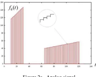
2) An orthogonal basis

A discrete signal is acquired by an Analog Digital Converter (ADC) on a regular sampling time t . The signal can be represented by the vector _n x(n) or by the sequence

→ ),...} 2 ( ), 1 ( ), 0 ( ), 1 ( {..., )} ( {x n = x − x x x with t_n = n n∈ Z.

In turn a vector can be converted to an analog signal with a Digital Analog Converter (DAC) (see Fig. 2a).

) (

0 t

f

Figure 2a. Analog signal.

The signal in Fig.2a can be represented by a sum of translated first-order cardinal B-spline functions φ(t) also called “box function” (see Fig. 2b) defined by

) (t

φ = 1 for 0≤ t<1

0 otherwise.

For example the signal f₀(t) (see Fig. 2a) can be written as k N k N k k N k

k

r

k

m

k

l

t

f

(

)

[

∑

(

)

∑

(

)]

φ

∑

(

)

φ

=

+

=

The ‘box functions” are an orthonormal basis (Haar basis). Indeed we have

. (2.1) k m m k dt m t k t

φ

φ

φ

δ

φ

∫

where δ_pk is the usual Kronecker delta symbol.

δ

k

=

m

2 ( t_j −k

φ the scale is proportional to 2−j.

Remark that the equality (2.1) remains valid if we change the scale k m m j k j

φ

δ

φ

>=

<

|

To change the scale wich we analyse a signal, we need to study the relation existing between the function φ(t) and its dilation.

2.1) The dilation equation

For the “box function” the dilation equation is ) 1 2 ( ) 2 ( ) (t =

φ

φ

φ

=<φ φ , we can written the equation (2.1.1) as ) 2 ( ) ( 2 ) ( 1 0 k t k h t k − =

∑

Let V the Hilbert subspace spanned by _m )} 2

( t_m −k φ

2.2) The Haar wavelet

Some signals created by a DAC (see Fig. 2c) can better represented by a sum of functions with a zero mean value called wavelet.

Figure 2c. Analog signal.

The Haar wavelet is defined by the function w(t)(see Fig. 2.2a) with w(t)=1 for 2 1 0≤ t < andw(t)=−1 for 1 2 1 < ≤ t .

Figure 2.2a. Haar wavelet. We have a relation between φ( t2 ), )φ(2t−1 and the new function w(t)

) 1 2 ( ) 2 ( ) (t = t − t− w φ φ . (2.2.1)

If we set ( )| (2 ) (0) 2 1 g t t w >= =< φ and ( )| (2 1) (1) 2 1 g t t w − >= =<

− φ , we can written the

equation (2.2.1) as ) 2 ( ) ( 2 ) ( 1 0 k t k g t w k − =

∑

The Haar wavelets also are an orthonormal basis. Indeed we have

>

=<

=

−

−

∫

∫

w

t

k

w

t

m

dt

w

w

dt

w

w

(

)

(

)

|

δ

k

=

m

The equality (2.2.2) remains valid if we change the scale k m m j k j

w

w

>=

δ

<

|

Let W the Hilbert subspace spanned by _m )} 2

( t k w

m −

{ with k∈Z.

Moreover there is a significant relation between the scale function φ(t) and the wavelet ) (t w

0

|

)

(

)

(

=

∫

=<

>=

∫

φ

t

w

t

dt

φ

w

dt

φ

w

0

|

,

>=

<

φ

w

The signal d₀(t) created by a DAC (see Fig. 2c) can be written with the Haar wavelet as

k N k k N k N k w k s w k q k p t d _0, 123 0 0 , 0 31 11 121 65 0 0 0( ) [

∑

∑

∑

3) The multiresolution analysis

In this section, we are going to show how we can represent a signal as a series of coarser and coarser approximation. Recall that the most basic level, a sampled signal{ is an approximation of the analog input signal (see Fig. 3a).

)} ( 0 n f ) (t f

Figure 3.a. Discrete signal.

The concept of approximation is rigorously defined with what that one calls the resolution. Intuitively, the higher the resolution, the better the approximation.

Definition 1. “For a finite length signal, the resolution is the minimum number of samples required to represent it”. [15]

Example: for N =128=27 the resolution is: 2 . 7

Given the vector { , the process by wich we keep only half the components,

, is called down- sampling by a factor two. Obviously, down-sampling reduces the resolution and creates a coarser approximation. Using this idea, we can apply a succession of digital filters to a signal while keeping the storage usage constant. For example, given the vector { , we can apply both a low-pass filter and a high-pass filter.

)} ( 0 n f )} )} 2 ( {f₁ n ( 0 n f

1) Apply a low-pass filter and down-sample the result by a factor of two. The result noted {f₁(2n)}can be seen as an approximation to {f₀(n)}.

2) Apply a high-pass filter and down-sample the result once again. The resulting vector is often described as containing the details of the signal and we note it {d₁(2n)}.In turn the filtered and down-sample approximation {f₁(2n)}can be decomposed with a low-pass and a digital high-pass filter and so on (see Fig. 3.b). This process will progressively reduce the resolution and create coarser and coarser approximations. We call this iterative process a wavelet transform (WT).

Figure 3.b. Wavelet transform.

3.1) The digital low-pass filter

We study the simplest low-pass digital filter: the moving average

) 1 ( 2 1 ) ( 2 1 ) ( _{0 0} 1 n = f n + f n+ f .

It can represent by a Toeplitz matrix [13]

                                =                 ) ( . . ) 1 ( ) 0 ( ) 1 ( ) 0 ( . . . . ) 1 ( ) 0 ( ) 1 ( ) 0 ( ) ( . . ) 1 ( ) 0 ( 0 0 0 1 1 1 N f f f h h h h h h N f f f .

The coefficients of the filter are

2 1 ) 1 ( ) 0 ( = h = h . For f₀(n) =e−in2πx we have x in x in x i x n i x in e x H e e e e n f₁ 2π ( 1)2π (1 2π ) 2π ( ) 2π 2 1 2 1 2 1 ) ( = − + − + = + − − = −

Where the frequency responseH(x) is

x i e x x H( ) =cos(

π

3.1.1) The down-sampling

We shall have only the even-numbered component of the output vector{ . The odd-numbered components are removed

)} ( 1 n f ),...} 4 ( ), 2 ( ), 0 ( ), 2 ( {..., )} 2 ( ){ 2 ( ) ( 1 1 1 1 1 1 m f n f f f f f = ↓ = − .

The symbol indicates down-sampling or decimation. We multiply the surviving components { by

↓

f₁(2n)} 2 to keep the l₂norm constant.

                = ↓ = ) 1 ( ) 0 ( . . . . ) 1 ( ) 0 ( ) 1 ( ) 0 ( ) 2 ( c c c c c c C L .

The coefficients of the filter are

2 ) 1 ( 2 ) 0 ( 2 1 ) 1 ( ) 0 ( c h h c = = = = .

This new vector{ can be in turn filtered and down-sampled (we call this

vector{ ). It is possible to continue this process until the number of points is one. We have represented this process for two-step at the Fig. 3c (for similar figures see [2]).

)} ( 1 m f )} ( 2 l f

The vectors{ ,{ , { contain the coefficients of respective

approximations in the Hilbert subspaces V . These subspaces satisfy the following relation )} ( 0 n f f₁(m)} f₂(l)},... ,... , , _{1 2} 0 V V 0 1 2 3 4 ...⊂V ⊂V ⊂V ⊂V ⊂V . (3.1.1)

3.2) The high-pass filter

We study the simplest high-pass digital filter: the moving difference. This filter is the mirror of the low-pass

) 1 ( 2 1 ) ( 2 1 ) ( _{0 0} 1 n = f n − f n+ d .

It can represent by a Toeplitz matrix.

                                =                 ) ( . . ) 1 ( ) 0 ( ) 1 ( ) 0 ( . . . . ) 1 ( ) 0 ( ) 1 ( ) 0 ( ) ( . . ) 1 ( ) 0 ( 0 0 0 1 1 1 N f f f g g g g g g N d d d .

The coefficients of the filter are

2 1 ) 0 ( = g and 2 1 ) 1 ( =− g . For f₀(n) =e−in2πx we have x in x in x i x n i x in e x G e e e e n d₁ 2π ( 1)2π (1 2π ) 2π ( ) 2π 2 1 2 1 2 1 ) ( = − − − + = − − − = −

and so the frequency responseG(x) is

x i e x i x G( )= sin(

π

3.2.1) The down-sampling

We keep only half output vector{ ; the odd-numbered components are removed and we multiply the surviving vector{ by

)} ( 1 n d )} 2 ( 1 n d 2 ),...} 4 ( ), 2 ( ), 0 ( ), 2 ( {..., )} ( ){ 2 ( ) ( 1 1 1 1 1 1 m d n d d d d d = ↓ = − .

                = ↓ = ) 1 ( ) 0 ( . . . . ) 1 ( ) 0 ( ) 1 ( ) 0 ( ) 2 ( d d d d d d D B

The coefficients of the filter are (0) 2 2 1 ) 0 ( g d = = and (1) 2 2 1 ) 1 ( g d =− = .

The vector { contains the coefficients corresponding to the Hilbert subspace W . It encodes the difference between the input vector {

)} ( 1 m d ₁ 0 0(n)} V

f ∈ and the vector {f₁(m)}∈V₁ (see Fig. 3d).

Figure 3d. Down-sampling (high-pass filter).

where the same signal is represented by coefficients at different scales. Typically, multiresolution is achieved by using a filter bank (set of filters).

Remark:

We have the relation

0 1 2 3 4 ...⊂V ⊂V ⊂V ⊂V ⊂V . (3.1) “There exist many ladders of spaces satisfying (3.1) that have nothing to do with “multiresolution”; the multiresolution aspect is a consequence of the additional requirement” [3] 0 )} 2 ( { )} ( {f n ∈V_j ⇔ f jn ∈V .

A multiresolution can be useful in itself. However, because we required orthogonality and perpendicularity of our basis function, we also have an inverse transform making it possible achieve perfect reconstitution of the signal.

3.2) The synthesis bank

The matrix representation for this operation is

                                =                 ) ( . . ) 1 ( ) 0 ( . 1 0 . . 0 0 1 . . . . . . . . . . . 1 0 0 . . 0 1 ) ( . . ) 1 ( ) 0 ( 0 0 0 0 0 0 N f f f N f f f .

We have the matrix annotation [f₀]=[I].[f₀] where [I] is the unit matrix.

Using the vector {d₁(m)}∈W₁ and the vector {f₁(m)}∈V₁, one can reconstitute the vector . Between the Hilbert subspaces V ,W and the Hilbert space V , we have the relation 0 0( )} {f n ∈V _{1 1 0} 1 1 0 V W V = ⊕ . For all j , we have

j j

j V W

We have represented the process of the exact reconstitution for two steps (see Fig. 3.2a).

Figure 3.2a. Exact reconstitution.

The analysis filter bank can be represented by the rectangular matrices L=(↓2)C

                = ↓ = ) 1 ( ) 0 ( . . . . ) 1 ( ) 0 ( ) 1 ( ) 0 ( ) 2 ( c c c c c c C L

and B=(↓2)D                 = ↓ = ) 1 ( ) 0 ( . . . . ) 1 ( ) 0 ( ) 1 ( ) 0 ( ) 2 ( d d d d d d D B .

We can write the low-pass matrix Land the high-pass matrixB in a same square matrix

] [ ) 2 ( ) 2 ( A D C B L =       ↓ ↓ =       .

The perfect reconstitution is possible because there is a corresponding inverse square matrix[A]−1called synthesis bank

[

]

[

]

The vectors { and { have half the component of { . To multiply by two the number of components, we insert a zero between each component of { and

. We call this process the up-sampling. It is represent by the symbol ↑ . To filter this operation we use the same filters that for the analysis. “The synthesis bank also has two steps, the up sampling and the filtering”. [13]

)} ( 1 m d f₁(m)} f₀(n)} )} ( 1 n d )} ( {f₁ n

Explicitly, the synthesis bank is given by the low-pass filter

                          = ↑ = ) 1 ( ) 0 ( . . ) 1 ( ) 0 ( ) 1 ( ) 0 ( ) 2 ( c c c c c c C LT

and the high-pass filter                           = ↑ = ) 1 ( ) 0 ( . . ) 1 ( ) 0 ( ) 1 ( ) 0 ( ) 2 ( d d d d d d D BT .

4) The denoising and the algorithms in ANSI C

The solution that we adopted is called the wavelet de-noising by thresholding. Recall that the process is as follows:

1) we give the algorithm for DWT;

2) we give the algorithm to identify and cut the noise in the wavelet domain; 3) we give the algorithm for the IDWT.

4.1) The DWT

To simplify the implementation, instead of using the square matrix [ from section 3.2

,

we use the equivalent matrix

] A                           = ) 1 ( ) 0 ( ) 1 ( ) 0 ( . . . . ) 1 ( ) 0 ( ) 1 ( ) 0 ( ) 1 ( ) 0 ( ) 1 ( ) 0 ( ] [ ~ d d c c d d c c d d c c A .

In language ANSI C we have /* coefficients for the scale */

const float Da1_scle[2] = { 0.7071067811865, 0.7071067811865 }; /* coefficients for the wavelet */

/* Haar */ /* ===== */

void fast_daubech1 ( int half, int PO_MEM_WAVEL, int PO_MEM_SCALE, int LS_MEMO_DWT) {

int kapa;

for (kapa = 0; kapa < half; kapa++){ signa [LS_MEMO_DWT + kapa] =

signa [ (2 * kapa) + PO_MEM_SCALE ] * Da1_scle[0] + signa [ (2 * kapa) + PO_MEM_SCALE + 1] * Da1_scle[1] ; signa [PO_MEM_WAVEL + kapa] =

signa [ (2 * kapa) + PO_MEM_SCALE ] * Da1_wavl [0] + signa [ (2 * kapa) + PO_MEM_SCALE + 1] * Da1_wavl [1] ; } /* end for (kapa = 0; kapa < half; kapa++) */

}/* end fast_daubech1 */ Remark:

The variable “half “is number of coefficients for the vectors { and . j j k W d ( )}∈ j j k V f ( )}∈ {

The variable “PO_MEM_SCALE »is the position in the memory, for the vector .

1 1( )}

{f_j− k ∈V_j−

The variable « LS_MEMO_DWT »is, in the memory, the position for the filtered (with the low-pass filter) and down-sampled vector {f_j(k)}∈V_j.

The variable « PO_MEM_WAVEL »is, in the memory, the position for the filtered (with the high-pass filter) and down-sampled vector {d_j(k)}∈W_j.

4.2) The IDWT

Again, to simplify the implementation, we use the equivalent matrix                           = − ) 1 ( ) 1 ( ) 0 ( ) 0 ( . . . . ) 1 ( ) 1 ( ) 0 ( ) 0 ( ) 1 ( ) 1 ( ) 0 ( ) 0 ( ] [ 1 ~ d c d c d c d c d c d c A .

In language ANSI C we have /* Invert Haar */

/* ========= */

void inv_daubech1 ( int half, int NXT_SCALE_IDWT, int PO_MEM_SCALE, int PO_MEM_WAVEL) {

int kapa;

for (kapa = 0; kapa < half; kapa++){

signa [NXT_SCALE_IDWT + ( 2 * kapa )] +=

signa [PO_MEM_SCALE + kapa] * Da1_scle[0] + signa [PO_MEM_WAVEL + kapa] * Da1_wavl [0]; signa [NXT_SCALE_IDWT + 1 + ( 2 * kapa )] +=

signa [PO_MEM_SCALE + kapa] * Da1_scle[1] + signa [PO_MEM_WAVEL + kapa] * Da1_wavl [1]; } /* end for (kapa = 0; kapa < half; kapa++)*/

} /* end inv_daubech1 */ Remark:

The variable “half ” is the number of coefficients for the vectors { and . j j k W d ( )}∈ j j k V f ( )}∈ {

The variable “NXT_SCALE_IDWT» is the position in the memory, the for the vector .

1 1( )}

{f_j− k ∈V_j−

The variable « PO_MEM_SCALE» is, in the memory, the position for the filtered (with the low-pass filter) and up sampled vector {f_j(k)}∈V_j.

The variable « PO_MEM_WAVEL » is, in the memory, the position for the filtered (with the high-pass filter) and up sampled vector {d_j(n)}∈W_j.

4.3) The denoising

While the energy of the noise will often spread itself over all wavelet coefficients,

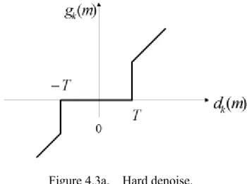
especially if the noise is white, the energy of the noise-free signal will usually only use few coefficients. To de-noise the signal, it is often sufficient to remove the coefficients with small amplitude and calculate the IDWT. We have chosen the hard thresholding approach [4] (see Fig. 4.3a). The hard tresholding is implemented with

T m g if T m g if m d T m g k k k k _< >    = = | ) ( | | ) ( | 0 ) ( ) ( ) ( ρ .

The de-noised vector is{g_k(m)} and {d_k(m)}the input vector.

Figure 4.3a. Hard denoise.

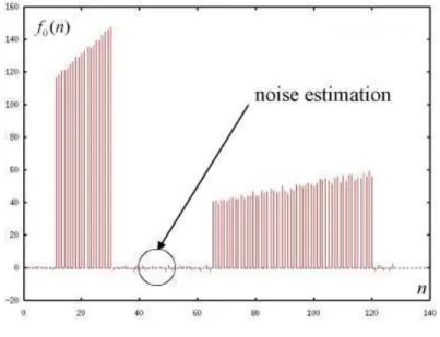
The threshold estimated by the formula T =Cσ 2.log_eN [4] , with σ = the noise standart deviation estimated by the formula

) ( 1 1 0

∑

∑

N = total number of samples = 20

C = constant. We have choice C, by a empirical method C =2,

is computed, always at the same time, using a short window in the original signal where we have the noise only (see Fig. 4.3b).

Figure 4.3b. Noise estimation.

In language ANSI C we have /* Hard denoise*/

void Hard_denoise ( int half, int PO_DEN_WAVEL, float TRESHOLD_VAL){ int kapa;

for ( kapa = 0; kapa < half; kapa++) {

if _ABS (signa [ PO_DEN_WAVEL + kapa] ) <= TRESHOLD_VAL) { signa [ PO_DEN_WAVEL + kapa] = 0.0;

} /* end if */

} /* end for ( kapa = 0; kapa < half; kapa++) */

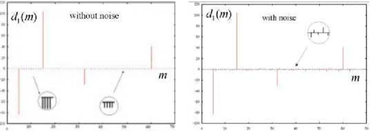
Respectively, we have represented at the figures Fig. 4.3c, Fig. 4.3d, Fig. 4.3e the vector { when the input signal is noise-free, when we add a noise and when we subtract the noise.

1 1(m)} W

d ∈

Figure 4.3c. {d₁(m)}Without noise. Figure 4.3c. {d₁(m)}With noise.

Remark:

With a classical filtering (Bessel, Butterworth, Tchebitchef low-pass, high pass or band-pass etc.), we reduce all the frequencies before or after the cut-off frequencie(s). It is not the case for wavelet shrinkage.

In Fig. 4.3f, we show the input vector {f₀(n)} when we add a noise.

Figure 4.3f. Input vector with noise.

In Fig. 4.3g, we have represent the input vector { when we apply the hard denoising for the vector{ .

)} ( 0 n f )} ( 1 m d

In Fig. 4.3h, we show the input vector {f₀(n)} when we apply the hard de-noising for the vectors{d₁(m)} and {d₂(l)}.

Figure 4.3h. With de-noising for {d₁(m)} and {d₂(l)}.

In Fig. 4.3i, we show the input vector {f₀(n)} when we apply the hard de-noising for the vectors{d₁(m)},{d₂(l)}and {d₃(k)}.

5) Application

We have installed our software as a single file called “filt.c” in the DSC DLN3TRA1 (LINAC III) and in the DSC DPSBBDI (PSB injection). This file filter 2048 bytes created by a Struck ADC 755 and send the filtered data (1800 bytes) and row data (1800 bytes) to a sampler.

The characteristics of the DSC are VME Power PC 603E

CPU CES RIO 8062 (32 bits). Frequency clock: 200 MHz.

32 Mbytes RAM with no cache L2.

We don’t use optimisation (DEBUG = - g). All the process use 5 ms but with full optimisation (DEBUG = - 02). It possible to reduce the execution time by two. Remark:

A DSC is the generic name (Device Stop Controller) used for VME-based front-end computers. These computers embed a local CPU (single unit VME) running the real-time OS Lynxos. This is used to drive various kind of equipment (e.g. field bus like GPIB, MIL1553, CAN, or data acquisition cards.

In Fig. 5a, we show the raw data and the filter data for the transformer ITH.MTR41.

In Fig. 5b, we show the details for the calibration of ITH.MTR41.

Figure 5b. Calibration of ITH.MTR41

In Fig. 5c, we show the raw data and the filter data for the transformer ITH.MTR15

We have measured the characteristics of the noise for the data filtered and no filtered for a typical transformer used to measure the beam injection in the PSB: the transformer

BI.TRA10 (see respectively TAB 1 and TAB2):

Column1 Column1

Mean 0.62 E+09 ions Mean 0.72 E+09 ions

Standard Error 14.80 Standard Error 17.21

Median 0.67 E+09 ions Median 0.56 E+09 ions

Standard Deviation 1.40 E+09 ions Standard Deviation 1.72 E+09 ions

Kurtosis 0.87 Kurtosis 0.09

Skewness 0.17 Skewness 0.03

Minimum -3.1 E+09 ions Minimum -3.7 E+09 ions

Maximum 4.5 E+09 ions Maximum 4.9 E+09 ions

Count 100 Count 100

With de-noising. Without de-noising.

TAB 1. TAB2.

With the wavelet de-noising we have reduce the standard deviation by≈ . While we compensated for some errors sources, other remains such as imperfect base line correction and also imperfect calibration. Thus, it might be that the only solution remaining to

improve further the signal would be to upgrade the sensor.

% 14

6) Conclusion:

The wavelet shrinkage is not really a solution for all noise–related problems. We have show that it can make a significant difference and we hope to promote further its use in the CERN engineering community. The best de-noising technique will always depend on the characteristics of the signal. In wavelet de-noising, one needs to choose the best wavelet basis and this choice warrants further research.

Acknowledgment

We would like to thanks Monsieur Pierre de Ronsard (French poet 1524-1585). Who was the first person ever to “see” a wavelet and who allowed us to imagine women’s smiles in the fold of the roses.

References :

[1] N.Angert (GSI), M.P Bougarel (GANIL), E. Brouzet, R. Cappi , D. Dekkers, J. Evans, G. Gelato, H. Haerot, C.E. Hill, G. Hutter (GSI), J. Knot, H. Kulger, A. Lombardi (INFN, Legnaro), H. Lustig, E. Malwitz (GSI), F. Nitsh, G. Parisi (INFN, Legnaro), A. Pissent (INFN, Legnaro), U. Raich, U. Ratzinger (GSI), L. Riccati (INFN, Torino), A. Schempp (IAP, Frankfurt), K. Schindl, H. Schönauer, P. Têtu, H.H.

CERN Report 93-01, Geneva, 1993.

[2] B. Bourrel, Calcul récursif de frame inverse sur la transformée en ondelettes dyadique,technical report, Ecole des mines de Paris, 2000.

Available at http://cas.ensmp.fr/~chaplais/FTP/Preprints/FrameInverse-e.pdf.

[3] I. Daubechies, Ten lectures on wavelets, CBMS-NSF Regional conference series in applied mathematics, SIAM 1992.

[4] D. Donoho and I. Johnstone, Ideal spacial adaptation via wavelet shrinkage , Biometrika, 81(3), 425-455, 1994.

[5] G. Gelato, The measurement of the charge injected into the PSB, BD note, 95-06. [6] Haar, Zur Theorie der orthogonalen Funktionen-system, Math. Ann, 69, pp 331-371,

1910.

[7] D. Lemire, G.Deslauriers, and S.Dubuc, Exemples simples de débruitage de

signaux courts par ondelettes, Séminaire de mathématiques appliquées,Université de Montréal, Montréal , Canada, 1997.

[8] F.Lenardon, J-D Schnell, S. Tirard, Les transformateurs rapides pour les ions plomb, PS/BD/Note 2000-06.

[9] F.Nanni, A beam transformer with a very wide range of sensitivity, PS/BD/Note 98-02. [10] S. Dubuc and G. Deslauriers, Spline functions and the theory of wavelets,

CRM Proceedings & lectures notes, Vol 18, AMS, 1999.

[11] S. Mallat, A wavelet tour of signal processing, Academic press, 1998.

[12] L. Råde and B. Westergren, Mathematics handbook for Science and Engineering, Springer, 1999.

[13] Gilbert Strang and Truong Nguyen, Wavelets and filter banks, Wellesley-Cambridge Press, 1997.

[14] Robert. M. Young , An introduction to Non Harmonic Fourier series, Academic press,2000.