Calibration of Dynamic Traffic Assignment
Models with Point-to-Point Traffic Surveillance
The MIT Faculty has made this article openly available. Please share
how this access benefits you. Your story matters.
Citation
Vaze, Vikrant, Constantinos Antoniou, Yang Wen, and Moshe
Ben-Akiva. “Calibration of Dynamic Traffic Assignment Models with
Point-to-Point Traffic Surveillance.” Transportation Research
Record: Journal of the Transportation Research Board 2090, no. 1
(July 30, 2009): 1–9.
As Published
http://dx.doi.org/10.3141/2090-01
Publisher
Transportation Research Board of the National Academies
Version
Final published version
Citable link
http://hdl.handle.net/1721.1/89062
Terms of Use
Article is made available in accordance with the publisher's
policy and may be subject to US copyright law. Please refer to the
publisher's site for terms of use.
tors. Coifman and Krishnamurthy used dual loop detectors to re-identify vehicles at downstream locations by matching their lengths to estimate path travel times (4). Wilson used a vehicle reidentifica-tion algorithm to create individual vehicle trajectories that use a series of loop detectors with sufficiently small spacing (5).
Mahanti focused on calibration of both demand and selected sup-ply parameters for the MITSIMLab microscopic simulator by formu-lating the overall optimization problem in a generalized least-squares (GLS) framework (6). The approach divides the parameter set into two groups, origin–destination (O-D) flows and the remaining param-eters, and an iterative solution method is implemented; the O-D flows are estimated by using the classical GLS estimator, and the parameters are estimated by using Box complex iterations (7 ). Balakrishna formulated the offline calibration framework as a large-scale optimization problem in which the final objective is to match simulated and observed quantities (8). Gupta demonstrated the cal-ibration of the mesoscopic dynamic traffic assignment (DTA) model DynaMIT by using separate methodologies to calibrate the demand and supply parameters sequentially (9).
Kunde presented the calibration of supply models within a meso-scopic DTA system (10). A three-stage approach to supply calibra-tion is outlined, in increasing order of complexity (single segment, subnetwork, entire network). The results in the networkwide calibra-tion show that the simultaneous perturbacalibra-tion stochastic approxima-tion (SPSA) algorithm provides results comparable to those of the Box complex algorithm by using a much lower number of function evaluations, thus requiring much less run time.
Ashok introduced the notion of direct measurements for the incor-poration of probe vehicle information for the solution of the O-D esti-mation and prediction problem (11). Van der Zijpp combined volume counts with trajectory information obtained from automated license-plate surveys for the estimation of O-D flows (12). Mishalani et al. evaluated the role of various types of surveillance data in the real-time estimation of dynamic O-D flows at the intersection level (13).
Oh and Ritchie developed a methodology for the design of advanced traffic surveillance systems based on microscopic traffic simulation (14). They demonstrated the proposed methodology through the development of an inductive-signature-based anonymous vehicle tracking system for the O-D flow estimation problem.
Dixon and Rilett proposed a method for using sample link choice proportions and sample O-D matrix information derived from AVI data sampled from a portion of vehicles to estimate population O-D matrices with the AVI data collection points acting as the origins and the destinations (15).
Kwon and Varaiya developed a statistical O-D estimation model by using partially observed vehicle trajectories obtained with vehicle reidentification or AVI techniques such as electronic tags (16).
Calibration of Dynamic Traffic
Assignment Models with
Point-to-Point Traffic Surveillance
Vikrant Vaze, Constantinos Antoniou, Yang Wen, and Moshe Ben-Akiva
1 Transportation Research Record: Journal of the Transportation Research Board, No. 2090, Transportation Research Board of the National Academies, Washington, D.C., 2009, pp. 1–9.
DOI: 10.3141/2090-01
Accurate calibration of demand and supply simulators within a dynamic traffic assignment system is critical for consistent travel information and efficient traffic management. Emerging traffic surveillance devices such as automatic vehicle identification (AVI) technology provide a rich source of disaggregated traffic data. A methodology for the joint calibra-tion of demand and supply model parameters using travel time measure-ments obtained from these emerging traffic-sensing technologies is presented. The calibration problem has been formulated as a stochastic optimization framework. Two different algorithms are used for solving the calibration problem: a gradient approximation–based path search method and a random search metaheuristic. The methodology is first tested by using a small synthetic study network to illustrate its effective-ness and obtain insight into its operation. The methodology is further applied to a real traffic network in Lower Westchester County, New York, to demonstrate its scalability. The estimation results are tested by using a calibrated microscopic traffic simulator. The results are com-pared with the base case of calibration by the use of only the conventional point sensor data. The results indicate that use of AVI data significantly improves calibration accuracy.
Previous and ongoing research shows the effectiveness of individual vehicle detection and identification techniques for improved traveler information and traffic management. Ruhe et al. demonstrated the usability of airborne traffic imagery for individual vehicle detection and detailed forecasts of traffic speed, density, travel times, and queue lengths (1). Hickman and Mirchandani reviewed major developments in the field of airborne imagery for traffic flow measurement and its applications to estimation of individual vehicle trajectories (2). Bar-Gera used cell-phone-based probe vehicles to compare speed and travel time measurements with those obtained from loop detectors (3). The analysis suggests that vehicle identification data based on such emerging technologies appear to be suitable for advanced traveler information system (ATIS) applications.
Recent efforts have been made to generate individual vehicle paths by using conventional detection techniques such as loop
detec-V. Vaze, Y. Wen, and M. Ben-Akiva, Massachusetts Institute of Technology, Room 1-181, 77 Massachusetts Avenue, Cambridge, MA 02139. C. Antoniou, Laboratory of Transportation Engineering, Department of Rural and Surveying Engineering, National Technical University of Athens, 9 Iroon Polytechniou Street, Zografou 15780, Athens, Greece. Corresponding author: C. Antoniou, antoniou@ central.ntua.gr.
Antoniou et al. presented a methodology for the incorporation of AVI information into the O-D estimation and prediction frame-work (17 ), which was generalized into a flexible formulation that can incorporate a large range of additional surveillance informa-tion (18). Zhou and Mahmassani used a nonlinear ordinary-least-squares estimation model to combine AVI counts, link counts, and historical demand information and solved the O-D estimation as an optimization problem (19).
Balakrishna et al. developed an offline DTA model calibration methodology for simultaneous demand and supply parameter esti-mation that is easily extendable to incorporate other types of traffic sensor data (20). Two algorithms are used for optimization: SPSA and SNOBFIT. It is concluded that the two algorithms result in com-parable parameter estimates, although SPSA does so at a fraction of the computational requirements.
This paper formulates the DTA model calibration problem as an optimization problem that allows the use of multiple types of surveil-lance information as measurements. Particular emphasis is given to emerging surveillance technologies, such as those providing point-to-point travel time measurements. Candidate solution approaches are surveyed, and the most promising are selected and applied to a series of case studies.
PROBLEM FORMULATION
The general calibration problem involves estimation of O-D flows as well as various model parameters by using a variety of data from sensor measurements and a priori values of O-D flows and model parameters. The calibration problem can be described as an opti-mization problem with the objective of minimizing the goodness-of-fit measure comparing the observed and fitted measurement values. An alternative formulation is as a state–space model, where the state vector comprises the model inputs and parameters that need to be estimated (17, 18, 21). In this paper, the problem is formulated as an optimization problem.
The following notation is used to formulate the DTA calibration problem in the optimization framework:
t= time intervals; t ∈{1, 2, . . . , T}; x= O-D flows; x = {xt}, ∀t ∈{1, 2, . . . , T};
β = model parameters; β = {βt}, ∀t ∈{1, 2, . . . , T}; Mo= observed sensor measurements; Mo = {Mo
t}, ∀t ∈{1, 2, . . . , T};
xa= a priori O-D flows; xa= {xa
t}, ∀t ∈{1, 2, . . . , T};
βa= a priori model parameter values; βa = {βa
t},∀t ∈{1, 2, . . . , T};
G= road network characteristics; G = {Gt}, ∀t ∈{1, 2, . . . , T}; Ms= simulated sensor measurements; Ms = {Ms
t},∀t ∈{1, 2, . . . , T}; and
z= function representing goodness of fit between observed or a priori values and measured or true values.
With this notation, the general calibration problem can be expressed as minimization of the goodness-of-fit measure z subject to constraints as follows:
subject to the constraints Ms= f(x, β, G), l
x< x < ux, and lβ< β < uβ,
where lxand lβ are appropriate lower bounds and uxand uβare
upper bounds. minimize x s o a a z M x M x ,β ( , , ,β , ,β ) ( )1
2 Transportation Research Record 2090
The model parameters may include the trip choice model param-eters of the route, mode, departure time, and destination choice mod-els on the demand-side as well as the supply-side parameters. The supply-side parameters to be calibrated depend on the type of supply simulator. In the case of a microscopic supply simulator such as MITSIMLab (22, 23), they would include the parameters in micro-scopic driver behavioral models such as acceleration–deceleration, lane-changing, gap acceptance, and merging models. In the case of a mesoscopic supply simulator such as the one in DynaMIT (24), the supply parameters include the parameters of the speed–density curves of each segment in the network as well as segment capacities.
The general objective function can be split into three parts. The goodness of fit is often calculated separately for each of the three entities, that is, a priori model parameters, a priori O-D flows, and observed sensor measurements, and the overall goodness-of-fit mea-sure can be expressed as an additive function of individual fit values as follows:
The functions z1, z2, and z3represent the goodness of fit and are often
described by a sum of squared deviations for sensor measurements, O-D flows, and model parameters, respectively.
SOLUTION ALGORITHMS
Most algorithms that solve nonlinear optimization problems, such as Newton’s method (25), the steepest descent method (26, pp. 428–436), and the conjugate gradient method (27 ), make use of a gradient vec-tor to indicate the direction of cost reduction. These algorithms usu-ally assume a closed-form analytical objective function, the ability to calculate the gradient vector, and a deterministic setting, which are often unreasonable for practical problems. For example, for the problem at hand, the objective function depends on the output of a large-scale, stochastic, noisy simulator that does not have an analytical expression. Computing the gradient is therefore cumber-some. Each function evaluation is computationally expensive, as it involves a run of the simulator. Therefore, numerical derivatives become an impractical operation (from a computational point of view) for problems with realistic dimensions (hundreds or thousands of parameters to calibrate).
Various stochastic optimization techniques try to overcome these limitations. Stochastic approximation algorithms trace a sequence of points in the search space that ultimately converges to the point of zero gradient. The evolution vector θi+1at the beginning of the i+ 1th iteration of the algorithm is given by
where gˆ(θi) is the gradient approximation at the ith iteration and aiis the sequence of step-size parameters, also known as gain sequence.
The finite difference stochastic approximation (FDSA) approach calculates the gradient vector by perturbing each component of the parameter vector separately and hence—with n denoting the number of parameters to be calibrated—requires 2n+ 1 functional evaluations in each iteration. SPSA calculates the gradient vec-tor by simultaneous perturbation of all the components of the parameter vector, requiring only three function evaluations per iteration (28, 29). It can be shown that the overall convergence rate of SPSA approaches n times that of FDSA (30). Spall has
θi+1= −θi a giˆ( )θi ( )3 minimize x o s a a z M M z x x z ,β 1
(
,)
+ 2(
,)
+ 3(
β β,)
( )2extensively discussed the conditions for convergence of SPSA algorithm (28, 30–32).
In pattern search methods, such as the Hooke and Jeeves method (33) and Nelder and Mead’s downhill simplex (34), a pattern of function evaluations at various points in the response surface is used to obtain an improved solution at each iteration. Box proposed an extended version of the Nelder–Mead downhill simplex algorithm, which potentially can increase the speed and accuracy of the search and guards against the possibilities of numerical instabilities (7 ). Balakrishna provided a detailed exposition of the numerical problems associated with the Nelder–Mead approach (8). Mahanti provided a detailed description of the implementation details of the Box complex algorithm for the calibration of DTA models (6).
Path search methods start at an initial point in the search space and keep moving to improve the objective function value based on the gradient. Response surface methodology (RSM) (35) and sto-chastic approximation are two important families of path search methods. RSM involves local polynomial approximation of the sur-face at each iteration. SNOBFIT is an extension of the RSM, which begins with a population of several points in the search space, and the points are chosen on the basis of the lower and upper bounds on decision variable values (36).
Random search methods maintain a large set of points at each iter-ation and randomly select updated parameter vectors to improve toward optimality. Metaheuristics such as genetic algorithms (GAs) and simulated annealing fall into this category. GA techniques have been successfully implemented for calibration of microscopic traffic simulation tools (37– 40). GAs use techniques inspired by evolution-ary biology, such as inheritance, mutation, selection, and crossover. A population of abstract representations (called chromosomes) of candidate solutions evolves toward better solutions. The evolution usually starts from a population of randomly generated individuals. In each generation, the fitness of every individual in the population is evaluated, multiple individuals are probabilistically selected from the current population on the basis of their fitness (selection), are recombined (crossover), and are possibly mutated (mutation) to form a new population. The algorithm terminates when either a maxi-mum number of generations has been produced or a satisfactory fitness level has been reached for the population. The simplest form of GA involves three types of operator: selection, crossover, and mutation (41). Popular and well-studied selection methods are roulette-wheel selection and tournament selection. One-point crossover, two-point crossover, and cut-and-splice crossover are the common crossover techniques. The mutation operator allows ran-dom flipping of some bits in a chromosome. GA techniques were used to calibrate driver behavior parameters in the microscopic models CORSIM and TRANSIMS (42). Rathi et al. used GA to determine the best location for variable message signs in traffic net-works for optimal response to incidents (43). However, scalability can be an issue for expensive function evaluations (44). The choice of GA operators and the corresponding parameters is critical for the success of GA applications. As problem dimension increases (45), the required population size increases exponentially.
Simulated annealing mimics the natural process of cooling of met-als (46, 47 ). It can reach a global optimum because of high-energy initial movements that increase the probability of reaching a better solution. The method is effective for combinatorial optimization with discrete variables. The performance of simulated annealing with continuous variables is not encouraging (48).
Among the path search methods, SPSA is a notable candidate, as it reaches convergence with much lower computational effort.
Furthermore, it is highly successful in solving large-scale DTA (8) and microscopic traffic simulator (49) calibration problems and has been shown to outperform SNOBFIT (8). Poor convergence to the global optimum and difficulties in handling stochasticity reduce the attractiveness of pattern-search methods for application to the DTA calibration problem. Among the random search methods, GA has been successfully applied to microscopic model calibration in the context of transportation, whereas simulated annealing has been shown to have slower convergence. Therefore, SPSA and GA have been chosen as candidate algorithms for the case studies presented in this paper.
SETUP OF CASE STUDIES Objectives
The main objectives for the case studies are as follows:
• Demonstrate the feasibility and effectiveness of the proposed
DTA calibration approach involving utilization of AVI data;
• Evaluate the relative effectiveness of the simultaneous demand–
supply calibration compared with demand-only calibration; and
• Compare the numerical accuracy and computational
perfor-mance of the considered algorithms (i.e., SPSA and genetic algo-rithms) in a synthetic case study and demonstrate the scalability of the most suitable algorithm in a large-scale case study (involving a complex network with multiple vehicle classes and different link use restrictions for different classes).
DTA Model and Other Software
The DTA model used for the case studies is DynaMIT (24), a simulation-based, real-time system designed to generate consistent, anticipatory route guidance for transportation networks. Anticipa-tory information (based on predicted network states) has been shown to be effective in eliminating driver overreaction (50, 51). DynaMIT combines real-time surveillance data with historical data to esti-mate current network state, predict future traffic conditions, and gen-erate consistent and unbiased information. DynaMIT uses an algorithm to obtain consistent estimates of current and future states (52, 53).
For the purposes of the case studies presented in this paper, the AVI capabilities of DynaMIT were used to replicate a transponder-based system, such as the TRANSMIT (transponder-transponder-based electronic toll collection) system that operates in New York and New Jersey (54). However, since the TRANSMIT network in the study area was not fully operational, the operation of the system was simulated within a microscopic traffic simulator, MITSIMLab (22, 23). AVI market penetration was assumed to be 30%. The sensor measure-ments were obtained as the average of 10 MITSIMLab runs. For val-idation of the calibrated DynaMIT parameters, a single additional run of MITSIMLab was performed, and the sensor data were provided as input to the real-time estimation procedure within DynaMIT.
Study Networks
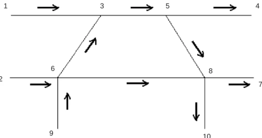
Two networks were used for the case studies presented in this paper. A synthetic network is used to gain insight into the performance of the two algorithms (Figure 1). The network consists of 10 nodes and
10 links, and traffic is loaded through six O-D pairs. The model is calibrated for a period of four 15-min intervals, a total of 1 h.
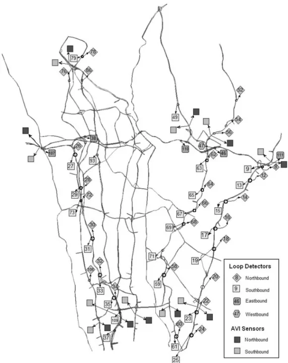
The second study network covers Lower Westchester County, just to the north of New York City (Figure 2) and includes the most-important highway corridors that connect Upstate New York and Connecticut to New York City. Since there are entry restrictions on the parkways in this region (no heavy commercial vehicles, such as trucks or trailers, may enter these facilities), the proportion of commer-cial vehicles in all O-D flows for each time interval is approximated on the basis of the average proportion of commercial vehicle observed during that time interval at three toll plazas in the area. The propor-tion of commercial vehicles in the traffic varies considerably with time. AVI sensors are located at 10 locations (shown in Figure 2), covering both southbound and northbound traffic. For each direc-tion of traffic, there are five upstream and five downstream sensors, allowing for 5 × 5 = 25 sensor (and thus travel time) pairs. There-fore, for both directions, 50 travel time observations per period are available. AVI sensors are not located on the border of the network and therefore do not provide any direct O-D measurements. Instead, they provide travel time measurements for the subpaths defined between any two sensors.
The study network consists of 1,767 links (split into 2,564 seg-ments) and 825 nodes. Traffic is loaded onto the network through 482 O-D pairs. The beginning of the morning peak (from 6:00 to 8:00 a.m.) was chosen as the simulation period. This period was divided into eight 15-min intervals. Aggregated sensor data are available for each of these 15-min intervals, and dynamic O-D flows are estimated for each interval. The number of demand parameters to be calibrated is therefore equal to 482 O-D pairs times eight intervals, that is, 3,856 parameters. For supply parameters, capacities are cali-brated for 2,564 segments. The segments were collected into 10 groups on the basis of similar traffic dynamics properties, and a single speed–density relationship was calibrated for each group. Within each speed–density relationship are five parameters to be calibrated, and thus there are 50 more parameters. Therefore, 3,856 O-D flows plus 2,564 segment capacities plus 50 speed–density parameters equals 6,470 parameters for joint demand-supply calibration.
Experimental Design
The following dimensions are considered in developing the experi-mental design for the case studies presented in this paper:
4 Transportation Research Record 2090
• Network
– Simple, synthetic network – Complex, large-scale network
• Scope of calibration
– Base case (using a priori available parameters and inputs; supply parameters come from a previous calibration for the spe-cific network, and demand parameters are perturbed randomly)
– Demand-only calibration, starting from the O-D flows used in the base case (using the a priori supply parameters from a pre-vious calibration of the same network)
– Joint demand and supply calibration, starting from the param-eter values used in the base case
• Surveillance data
– Link counts only
– Link counts and travel time (obtained from the AVI as the time difference between two successive detections of an AVI-equipped vehicle from different AVI sensors)
• Optimization algorithm
– SPSA – GA
Implementation Details
SPSA and GA are used. For each of these algorithms, several parameters are chosen on a case-by-case basis. To avoid ambiguity, the main implementation details are presented here. In the case of the SPSA algorithm, the jth component of gradient of objective function at the ith iteration is calculated as follows:
The next estimate of the parameter vector is then calculated as follows:
The feasible region for optimization is defined by the lower and upper bounds on each of the parameter values. A simple implemen-tation of the projection operator Πcis used such that whenever any component of the parameter vector is higher than the upper bound or lower than the lower bound, the projection operator sets it to the upper-bound and lower-bound values, respectively.
θi+1=Πc
[
θi−a Yi(
θi)
]
( )5 ˆ ˆ ˆ ˆ ( g f c f c c ij i i i i i i i j ij θ θ θ(
)
=(
+ iΔ)
−i(
− iΔ)
Δ 2 44) 1 3 2 6 8 7 9 10 5 4Appropriate values of the parameters of interest, a, c, alpha, and gamma, are critical for achieving convergence. Alpha and gamma are critical parameters since they determine the gain sequence. The recommended values for alpha and gamma are around 0.602 and 0.101 per the theoretical convergence conditions provided by Spall (29). By using a line-search approach, the values chosen were c= 1.9 and a= 20. Regarding the probability distribution of the compo-nents of the perturbation vector, the suggestion of a± 1 Bernoulli distribution is adopted.
Application of GAs involves more complex implementation deci-sions. Selection operator, crossover operators, and mutation opera-tor, as well as best parameter values, must be chosen. Parameter values are application specific, and therefore they were selected by
following a line-search procedure using the synthetic network (used in the first case study presented in the remainder of this paper). The number of particles (chromosomes) to be used is also an important decision. These decisions can considerably affect the computational performance and convergence rate of GAs. Therefore, various oper-ators were explored before the most suitable were chosen for the final calibration effort:
• For the selection step, roulette wheel selection was found to be
the best operator. In the roulette wheel selection operator, the prob-ability of selecting each chromosome is proportional to its fitness value. In this case, the fitness value is computed as the inverse of the objective function value at that point.
• The single-point crossover operator was chosen because of its
simplicity. It was deemed unnecessary to use complicated crossover operators such as two-point crossover. Some operators, such as cut-and-splice, cannot be used, since they change the dimension of the decision vector.
• The crossover parameter value was obtained through a line
search, and 0.7 was found to be the most suitable. This value is within the range of those indicated in the literature.
• The choice of mutation operator is a critical decision since
there is no direct equivalent of bit mutation in case of continuous variables. A novel approach was used for mutation: if a variable is to be mutated, its value is drawn from a uniform random distribu-tion with mean equal to the current value and the range from 0 to current value multiplied by 2.
• Based on a line-search procedure on the synthetic data set, the
value of the mutation parameter is 0.002, which again is within the range of values encountered in the literature.
• Finally, 100 particles (i.e., chromosomes) were used.
Most of these values are close to the empirically proved values suggested by de Jong (55). De Jong recommended use of 50 to 100 particles, a crossover rate of 0.6, and a mutation rate of 0.001 per bit. The population of 100 may appear quite low considering that the model in the case study in the large-scale network includes more than 6,000 parameters per interval. This choice is based on two considerations: obtaining a practical trade-off between compu-tational effort and calibration accuracy, and having comparable computational effort for the two algorithms, SPSA and GA, so that their performance can be compared in a more meaningful way.
Measures of Goodness of Fit
Five different statistics have been used to calculate the goodness of fit of the results (56, 57 ):
• Normalized root-mean-square error,
• Root-mean-square percent error,
• Root-mean-square error,
• Normalized mean error,
MEN= −
(
)
= =∑
∑
Y Y Y n s n o n N n o n N 1 1 RMSE= ⎡⎣ − ⎤⎦ =∑
1 2 1 N Yn Y s n o n N RMSPE= ⎡ − ⎣ ⎢ ⎤⎦⎥ =∑
1 2 1 N Y Y Y n s n o n o n N RMSN= −(
)
= =∑
∑
N Y Y Y n s n o n N n o n N 2 1 16 Transportation Research Record 2090
• Mean percent error,
Multiple statistics are used because they can capture different aspects of the obtained results. The normalized root-mean-square error and root-mean-square percent error quantify the overall error of the calibration. These measures penalize large errors at a higher rate than small errors. The root-mean-square error is a measure of the deviation of a simulated variable from its actual path. The normal-ized mean error measures the mean normalnormal-ized difference between simulated and observed values. The mean percent error statistic indicates the existence of systematic under- or overestimation in the simulated measurements. Percent error measures are often pre-ferred to their absolute error counterparts because they provide information on the magnitude of the errors relative to the average measurement.
RESULTS OF CASE STUDIES Synthetic Network
Two separate experiments were performed. First, only the demand was calibrated while supply was held constant. In the second experiment, demand and supply were calibrated simultaneously. Tables 1 and 2 summarize the results of the case study with the synthetic network. The demand-only calibration (which represents the state of the art in this field until a few years ago) provides consid-erable improvements and satisfactory results. The addition of AVI data leads to a further improvement. When both demand and sup-ply parameters are calibrated jointly, the accuracy of the calibration improves further.
A potential pitfall with calibration is overfitting the parameters to the specific data set. Validation (using a different set of data to ensure that the calibrated parameters are not overfit) provides a practical approach to check that overfitting has not occurred. A comparison of the two solution approaches indicates that SPSA outperforms GA. Therefore, SPSA with both link counts and AVI data is used for the validation, which suggests that the calibration has not led to overfitting of parameters to the particular data set.
Large-Scale Network
Table 3 presents the calibration and validation results for the Lower Westchester County network. On the basis of the findings of the syn-thetic network case study, the SPSA solution approach was selected for the case study. The calibration improves the fit of the model through estimation of the model parameters. The fit is better when both demand and supply parameters are calibrated. Similarly, use of both link counts and AVI information improves calibration results. The validation suggests that the calibrated parameters have not been overfit to the calibration data.
CONCLUSION
In this study, the problem of DTA model calibration using multiple data sources was formulated as a simulation-based optimization problem, which was solved by using two candidate algorithms,
MPE= ⎡ − ⎣ ⎢ ⎤⎦⎥ =
∑
1 1 N Y Y Y n s n o n o n NTABLE 1 Demand-Only Calibration Results for Synthetic Network
Starting
SPSA GA
Values Link Counts Counts + AVI Link Counts Counts + AVI
RMSN counts 32.49% 8.98% 10.35% 8.49% 9.15% RMSN TT 11.29% 9.52% 4.51% 10.04% 4.60% RMSPE counts 48.68% 15.77% 17.86% 15.51% 16.48% RMSPE TT 7.82% 6.59% 3.84% 6.98% 3.89% RMSE counts 144.32 39.88 45.98 37.69 40.62 RMSE TT 1.09 0.92 0.43 0.97 0.44 MEN counts 25.97% 3.85% 1.47% 1.63% 0.32% MEN TT 5.49% 2.86% 1.51% 1.33% 1.69% MPE counts 37.30% 7.79% 5.34% 5.51% 1.38% MPE TT 3.51% 1.96% 1.31% 1.10% 1.39%
NOTE: TT = travel times.
TABLE 3 Calibration and Validation Results for Lower Westchester County Network Using SPSA
Joint Demand–Supply Joint Demand–
Demand-Only Calibration Calibration Supply Validation
Starting Values Link Counts Counts + AVI Link Counts Counts + AVI Counts + AVI
RMSN counts 25.19% 20.09% 18.24% 20.69% 17.94% 17.63% RMSN TT 29.04% 22.23% 21.24% 19.46% 18.92% 18.55% RMSPE counts 28.54% 26.84% 30.32% 26.78% 28.92% 27.60% RMSPE TT 30.46% 22.43% 22.29% 23.89% 20.98% 21.06% RMSE counts 151.68 120.94 109.83 124.56 108.04 106.27 RMSE TT 219.17 167.79 160.30 151.07 147.10 148.67 MEN counts −12.15% −9.05% −6.61% −8.50% −3.87% −3.98% MEN TT 3.28% −7.59% −5.54% −9.00% −6.06% −9.88% MPE counts −7.43% −3.06% −0.37% −3.90% 0.16% −0.39% MPE TT 5.82% −2.74% −1.23% −3.49% −4.84% −5.15%
TABLE 2 Calibration and Validation Results for Synthetic Network
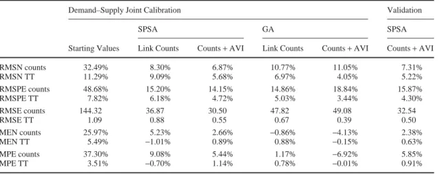
Demand–Supply Joint Calibration Validation
SPSA GA SPSA
Starting Values Link Counts Counts + AVI Link Counts Counts + AVI Counts + AVI
RMSN counts 32.49% 8.30% 6.87% 10.77% 11.05% 7.31% RMSN TT 11.29% 9.09% 5.68% 6.97% 4.05% 5.22% RMSPE counts 48.68% 15.20% 14.15% 14.86% 18.84% 15.87% RMSPE TT 7.82% 6.18% 4.72% 5.03% 3.44% 4.30% RMSE counts 144.32 36.87 30.50 47.82 49.08 32.54 RMSE TT 1.09 0.88 0.55 0.67 0.39 0.50 MEN counts 25.97% 5.23% 2.66% −0.86% −4.13% 2.38% MEN TT 5.49% −1.01% 0.89% 0.88% −0.15% 0.63% MPE counts 37.30% 9.08% 5.44% 1.17% −6.92% 5.85% MPE TT 3.51% −0.70% 1.14% 0.78% −0.01% 0.91%
applied to two different networks. Following are the main findings and conclusions:
• Simultaneous demand–supply calibration was found to be
superior to demand-only calibration, as it substantially increased calibration accuracy.
• A comparison of calibration results using combined loop
detec-tor and AVI data and calibration results using only loop detecdetec-tor data indicated that AVI data are useful for improving calibration accuracy in all the experiments. In this case study, the AVI data came from a very small number of sensors. Only 20 AVI sensors were assumed to provide data in the network, resulting in 50 travel time observations per interval, and the number of unknowns is 6,470.
• For the small network, SPSA was found to be the most
effec-tive algorithm, followed closely by GA. However, the GA’s perfor-mance required additional computational effort because of a greater number of required function evaluations.
• The empirical results from the validation tests were found to be
consistent with the calibration results and thus validated the feasibility and accuracy of the methods used for calibration in this research.
• The SPSA algorithm was found to be scalable. A large set of
parameters (6,470 parameters) was practically calibrated by using SPSA.
Directions for future research are as follows:
• Exploration of the effectiveness of a combination of travel
times and other types of AVI information, such as subpath flows and split fractions;
• Sensitivity analysis of market penetration and other key
parameters (e.g., number of AVI sensors);
• Effect of sensor location in calibration accuracy, as well as use
of additional information from probe or floating-car data; and
• Developing insight into the magnitude of various parameters of
solution algorithms.
REFERENCES
1. Ruhe, M., R. Kuehne, I. Ernst, S. Zuev, and E. Hipp. Airborne Systems and Data Fusion for Traffic Surveillance and Forecast for Soccer World Cup. Presented at 86th Annual Meeting of the Transportation Research Board, Washington, D.C., 2007.
2. Hickman, M., and P. Mirchandani. Airborne Traffic Flow Data and Traffic Management. Presented at Symposium on the Fundamental Diagram: 75 Years, Woods Hole, Mass., 2008.
3. Bar-Gera, H. Evaluation of a Cellular Phone-Based System for Measure-ments of Traffic Speeds and Travel Times. Transportation Research
Part C, Vol. 15, 2007, pp. 380–391.
4. Coifman, B., and S. Krishnamurthy. Vehicle Reidentification and Travel Time Measurement Across Freeway Junctions Using the Existing Detector Infrastructure. Transportation Research Part C, Vol. 15, 2007, pp. 135–153.
5. Wilson, R. E. From Inductance Loops to Vehicle Trajectories. Presented at Symposium on the Fundamental Diagram: 75 Years, Woods Hole, Mass., 2008.
6. Mahanti, B. P. Aggregate Calibration of Microscopic Traffic Simulation
Models. MS thesis. Massachusetts Institute of Technology, Cambridge,
2004.
7. Box, M. J. A New Method of Constrained Optimization and a Comparison with Other Methods. Computer Journal, Vol. 8, No. 1, 1965, pp. 42–52. 8. Balakrishna, R. Off-Line Calibration for Dynamic Traffic Assignment
Models. PhD thesis. Massachusetts Institute of Technology, Cambridge,
2006.
9. Gupta, A. Observability of Origin–Destination Matrices for Dynamic
Traffic Assignment. MS thesis. Massachusetts Institute of Technology,
Cambridge, 2005.
8 Transportation Research Record 2090
10. Kunde, K. K. Calibration of Mesoscopic Traffic Simulation Models for
Dynamic Traffic Assignment. MS thesis. Massachusetts Institute of
Technology, Cambridge, 2002.
11. Ashok, K. Estimation and Prediction of Time-Dependent
Origin-Destination Flows. PhD dissertation. Massachusetts Institute of
Tech-nology, Cambridge, 1996.
12. Van der Zijpp, N. J. Dynamic Origin–Destination Matrix Estimation from Traffic Counts and Automated Vehicle Identification Data. In
Trans-portation Research Record 1607, TRB, National Research Council,
Washington, D.C., 1997, pp. 87–94.
13. Mishalani, R. G., B. Coifman, and D. Gopalakrishna. Evaluating Real-Time Origin–Destination Flow Estimation Using Remote-Sensing-Based Surveillance Data. Presented at 82nd Annual Meeting of the Transportation Research Board, Washington, D.C., 2003.
14. Oh, C., and S. G. Ritchie. Development of Methodology to Design Advanced Traffic Surveillance Systems for Traffic Information Based on Origin–Destination. In Transportation Research Record: Journal
of the Transportation Research Board, No. 1935, Transportation
Research Board of the National Academies, Washington, D.C., 2005, pp. 37–46.
15. Dixon, M. P., and L. R. Rilett. Real-Time Origin–Destination Estima-tion Using Automatic Vehicle IdentificaEstima-tion Data. Presented at 79th Annual Meeting of the Transportation Research Board, Washington, D.C., 2000.
16. Kwon, J., and P. Varaiya. Real-Time Estimation of Origin–Destination Matrices with Partial Trajectories from Electronic Toll Collection Tag Data. In Transportation Research Record: Journal of the
Transporta-tion Research Board, No. 1923, TransportaTransporta-tion Research Board of the
National Academies, Washington, D.C., 2005, pp. 119–126.
17. Antoniou, C., M. Ben-Akiva, and H. N. Koutsopoulos. Incorporating Automated Vehicle Identification Data into Origin–Destination Estima-tion. In Transportation Research Record: Journal of the
Transporta-tion Research Board, No. 1882, TransportaTransporta-tion Research Board of the
National Academies, Washington, D.C, 2004, pp. 37–44.
18. Antoniou, C., M. Ben-Akiva, and H. N. Koutsopoulos. Dynamic Traf-fic Demand Prediction Using Conventional and Emerging Data Sources.
IEEE Proceedings Intelligent Transport Systems, Vol. 153, No. 1,
March 2006, pp. 97–104.
19. Zhou, X., and H. S. Mahmassani. Dynamic Origin Destination Demand Estimation Using Automatic Vehicle Identification Data. IEEE
Trans-actions on Intelligent Transportation Systems, Vol. 7, No. 1, 2006,
pp. 105–114.
20. Balakrishna, R., M. E. Ben-Akiva, and H. N. Koutsopoulos. Offline Calibration of Dynamic Traffic Assignment: Simultaneous Demand-and-Supply Estimation. In Transportation Research Record: Journal
of the Transportation Research Board, No. 2003, Transportation
Research Board of the National Academies, Washington, D.C., 2007, pp. 50–58.
21. Antoniou, C., M. Ben-Akiva, and H. N. Koutsopoulos. Nonlinear Kalman Filtering Algorithms for On-Line Calibration of Dynamic Traf-fic Assignment Models. IEEE Transactions on Intelligent Transportation
Systems, Vol. 8, No. 4, Dec. 2007, pp. 661–670.
22. Yang, Q., and H. N. Koutsopoulos. A Microscopic Traffic Simulator for Evaluation of Dynamic Traffic Assignment Systems. Transportation
Research C, Vol. 4, No. 3, 1996, pp. 113–129.
23. Yang, Q., H. N. Koutsopoulos, and M. E. Ben-Akiva. Simulation Labo-ratory for Evaluating Dynamic Traffic Management Systems. In
Trans-portation Research Record: Journal of the TransTrans-portation Research Board, No. 1710, TRB, National Research Council, Washington, D.C.,
2000, pp. 122–130.
24. Ben-Akiva, M. E., M. Bierlaire, D. Burton, H. N. Koutsopoulos, and R. Mishalani. Network State Estimation and Prediction for Real-Time Trans-portation Management Applications. Networks and Spatial Economics, Vol. 1, No. 3/4, 2001, pp. 293–318.
25. Ypma, T. J. Historical Development of the Newton-Raphson Method.
SIAM Review, Vol. 37, No. 4, 1995, pp. 531–551.
26. Arfken, G. The Method of Steepest Descents. In Mathematical Methods
for Physicists, 3rd ed. Academic Press, Orlando, Fla., 1985.
27. Hestenes, M. R., and E. Stiefel. Methods of Conjugate Gradients for Solving Linear Systems. J. Research Nat. Bur. Standards, Vol. 49, 1952, pp. 409–436.
28. Spall, J. C. An Overview of the Simultaneous Perturbation Method for Efficient Optimization. Johns Hopkins APL Technical Digest, Vol. 19, No. 4, 1998, pp. 482–492.
29. Spall, J. C. Implementation of the Simultaneous Perturbation Algorithm for Stochastic Optimization. IEEE Transactions on Aerospace and
Electronic Systems, Vol. 34, No. 3, 1998, pp. 817–823.
30. Spall, J. C. Stochastic Optimization, Stochastic Approximation and Simulated Annealing. In Wiley Encyclopedia of Electrical and
Elec-tronics Engineering (J. G. Webster, ed.), Wiley-Interscience, 1999,
pp. 529–542.
31. Spall, J. C. A Stochastic Approximation Algorithm for Large-Dimensional Systems in the Kiefer-Wolfowitz Setting. Proc., IEEE Conference on
Decision and Control, 1988, pp. 1544–1548.
32. Spall, J. C. Multivariate Stochastic Approximation Using a Simultaneous Perturbation Gradient Approximation. IEEE Transactions on Automatic
Control, Vol. 37, No. 3, 1992, pp. 332–341.
33. Kolda, T. G., R. M. Lewis, and V. Torczon. Optimization by Direct Search: New Perspectives on Some Classical and Modern Methods. SIAM
Review, Vol. 45, No. 3, 2003, pp. 385–482.
34. Nelder, J. A., and R. Mead. A Simplex Method for Function Minimization.
Computer Journal, Vol. 7, No. 4, 1965, pp. 308–313.
35. Kleijnen, J. P. C. Statistical Tools for Simulation Practitioners. Marcel Dekker, New York, 1987.
36. Huyer, W., and A. Neumaier. SNOBFIT: Stable Noisy Optimization by Branch and Fit. ACM Transactions on Mathematical Software, Vol. 35, No. 2, 2008.
37. Abdulhai, B., J. B. Sheu, and W. Recker. Simulation of ITS on the
Irvine FOT Area Using the PARAMICS 1.5 Scalable Microscopic Traffic Simulator. Phase I: Model Calibration and Validation. Report
UCBITS-PRR-99-12. PATH, Berkeley, Calif., 1999.
38. Lee, D.-H., X. Yang, and P. Chandrasekar. Parameter Calibration for PARAMICS Using Genetic Algorithm. Presented at 80th Annual Meeting of the Transportation Research Board, Washington, D.C., 2001. 39. Kim, K.-O. Optimization Methodology for the Calibration of
Trans-portation Network Micro-Simulation Models. PhD thesis. Texas A&M
University, 2002.
40. Kim, K.-O., and L. R. Rilett. Simplex-Based Calibration of Traffic Microsimulation Models with Intelligent Transportation Systems Data. In Transportation Research Record: Journal of the Transportation
Research Board, No. 1855, Transportation Research Board of the
National Academies, Washington, D.C., 2003, pp. 80–89.
41. Mitchell, M. An Introduction to Genetic Algorithms. MIT Press, Cam-bridge, Mass., 1998.
42. Kim, K.-O., and L. R. Rilett. Genetic Algorithm-Based Approach to Traffic Microsimulation Calibration Using ITS Data. Presented at 83rd Annual Meeting of the Transportation Research Board, Washington, D.C., 2004.
43. Rathi, V., C. Antoniou, M. Ben-Akiva, and Y. Wen. Optimal Variable Message Sign Location Identification Using Genetic Algorithms. Proc.,
10th ASCE Advanced Applications of Telematics in Transport Conference,
Athens, Greece, 2008.
44. Henderson, J. M., and L. Fu. Applications of Genetic Algorithms in Transportation Engineering. Presented at 83rd Annual Meeting of the Transportation Research Board, Washington, D.C., 2004.
45. Thierens, D. Scalability Problems of Simple Genetic Algorithms. Journal
of Evolutionary Computation, Vol. 7, No. 4, 1999, pp. 331–352.
46. Metropolis, N., A. W. Rosenbluth, M. N. Rosenbluth, A. H. Teller, and E. Teller. Equation of State Calculations by Fast Computing Machines.
Journal of Chemical Physics, Vol. 21, 1953, pp. 1087–1092.
47. Corana, A., M. Marchesi, C. Martini, and S. Ridella. Minimizing Multi-modal Functions of Continuous Variables with the Simulated Annealing Algorithm. ACM Transactions on Mathematical Software, Vol. 13, 1987, pp. 262–280.
48. Goffe, W. L., G. D. Ferrier, and J. Rogers. Global Optimization of Sta-tistical Functions with Simulated Annealing. Journal of Econometrics, Vol. 60, No. 1-2, 1994.
49. Balakrishna, R., C. Antoniou, M. E. Ben-Akiva, H. N. Koutsopoulos, and Y. Wen. Calibration of Microscopic Traffic Simulation Models: Methods and Application. In Transportation Research Record: Journal
of the Transportation Research Board, No. 1999, Transportation
Research Board of the National Academies, Washington, D.C., 2007, pp. 198–207.
50. Ben-Akiva, M., and I. Kaysi. Dynamic Driver Behavior Modeling for Advanced Driver Information Systems. Presented at 6th International Conference on Travel Behavior, Quebec, Canada, 1991.
51. Balakrishna, R., H. N. Koutsopoulos, M. E. Ben-Akiva, B. M. Fernando Ruiz, and M. Mehta. Simulation-Based Evaluation of Advanced Traveler Information Systems. In Transportation Research Record: Journal of
the Transportation Research Board, No. 1910, Transportation Research
Board of the National Academies, Washington, D.C., 2005, pp. 90–98. 52. Ben-Akiva, M. E., M. Bierlaire, J. Bottom, H. N. Koutsopoulos, and
R. Mishalani. Development of a Route Guidance Generation System for Real-Time Application. Proc., 8th IFAC Symposium on Transportation
Systems, Chania, Greece, 1997.
53. Bottom, J. A. Consistent Anticipatory Route Guidance. PhD thesis. Massachusetts Institute of Technology, Cambridge, 2000.
54. Mouskos, K. C., E. Niver, L. Pignataro, S. Lee, N. Antoniou, and L. Papadopoulos. TRANSMIT System Evaluation: Final Report. New Jersey Institute of Technology, Newark, 1998.
55. de Jong, K. A. An Analysis of the Behavior of a Class of Genetic Adaptive
Systems. PhD thesis. University of Michigan, Ann Arbor, 1975.
56. Pindyck, R. S., and D. L. Rubinfeld. Econometric Models and Economic
Forecasts, 4th ed. Irwin McGraw-Hill, Boston, Mass., 1997.
57. Toledo, T., and H. N. Koutsopoulos. Statistical Validation of Traffic Simulation Models. In Transportation Research Record: Journal of the
Transportation Research Board, No. 1876, Transportation Research
Board of the National Academies, Washington, D.C., 2004, pp. 142–150.
The Transportation Network Modeling Committee sponsored publication of this paper.