Planar Convex Hulls

https://doi.org/10.4224/8914427

READ THESE TERMS AND CONDITIONS CAREFULLY BEFORE USING THIS WEBSITE.

https://nrc-publications.canada.ca/eng/copyright

Vous avez des questions? Nous pouvons vous aider. Pour communiquer directement avec un auteur, consultez la première page de la revue dans laquelle son article a été publié afin de trouver ses coordonnées. Si vous n’arrivez pas à les repérer, communiquez avec nous à PublicationsArchive-ArchivesPublications@nrc-cnrc.gc.ca.

Questions? Contact the NRC Publications Archive team at

PublicationsArchive-ArchivesPublications@nrc-cnrc.gc.ca. If you wish to email the authors directly, please see the first page of the publication for their contact information.

NRC Publications Archive

Archives des publications du CNRC

For the publisher’s version, please access the DOI link below./ Pour consulter la version de l’éditeur, utilisez le lien DOI ci-dessous.

Access and use of this website and the material on it are subject to the Terms and Conditions set forth at

Planar Convex Hulls

Barton, Alan

https://publications-cnrc.canada.ca/fra/droits

L’accès à ce site Web et l’utilisation de son contenu sont assujettis aux conditions présentées dans le site LISEZ CES CONDITIONS ATTENTIVEMENT AVANT D’UTILISER CE SITE WEB.

NRC Publications Record / Notice d'Archives des publications de CNRC:

https://nrc-publications.canada.ca/eng/view/object/?id=585287e7-3c51-4269-a304-ce2c15aaf1c3

https://publications-cnrc.canada.ca/fra/voir/objet/?id=585287e7-3c51-4269-a304-ce2c15aaf1c3

National Research Council Canada Institute for Information Technology Conseil national de recherches Canada Institut de technologie de l'information

Planar Convex Hulls *

Barton, A.

November 2005

* published at NRC/ERB-1128. 4 Pages. November 2005. NRC 48290.

Copyright 2005 by

National Research Council of Canada

Permission is granted to quote short excerpts and to reproduce figures and tables from this report, provided that the source of such material is fully acknowledged.

National Research Council Canada Institute for Information Technology Conseil national de recherches Canada Institut de technologie de l'information

Pla na r Conve x H ulls

Barton, A.

November 2005

Copyright 2005 by

National Research Council of Canada

Permission is granted to quote short excerpts and to reproduce figures and tables from this report, provided that the source of such material is fully acknowledged.

ERB-1128

Planar Convex Hulls

Alan J. Barton

Integrated Reasoning Group Institute for Information Technology National Research Council Canada

Ottawa, Canada, K1A 0R6

alan.barton@nrc-cnrc.gc.ca

ABSTRACT

An attempt is made to understand some of the planar convex hull algorithms leading up to and including Chan’s 1995 planar convex hull algorithm. The algorithms include: i) Graham’s 1972 algorithm , ii) Jarvis’ 1973 algorithm, and iii) Chan’s 1995 algorithm.

Keywords

planar convex hull, design and analysis of algorithms, output-sensitive

1.

INTRODUCTION

We should not rely on careful examinations, we should avoid the need for it. – J.W. Tukey, 19771

Planar (2-dimensional) convex hulls may be used as a rep-resentation of the shape of a data set in application ar-eas of Pattern Recognition. For example, one application of using higher dimensional convex hulls is reported in [8]. There are other possible conceptualizations of the meaning for shape. One possibility is a generalization of the convex hull called an α-shape [7]. Higher dimensional convex hulls, input spaces other than R2, and other shape representations will not be discussed further.

The objectives are:

1. to find an efficient algorithm for constructing convex hulls, where the measure of efficiency is asymptotic worst-case running time as a function of both n (input size) and m (output size) [2], and

∗Report for the course COMP5730 entitled Design and Analysis of Algorithms at Carleton University

†Master of Computer Science (in progress)

1_{John W. Tukey was referring to the fact that plotted data}

(e.g. a scatter plot) should be clearly presented to a reader when attempting to argue for a particular perspective[6].

2. to report hull vertices in a counter clockwise ordering (not required, but convenient).

The following assumptions are made:

1. Each point, p, lies in an n = 2-dimensional space. 2. ∃ metric (d =Euclidian distance) defined over the space 3. When d = 2, no 3 points lie along the same line. If they do, perturbation methods could be used [2], but may introduce other problems. For example, points on the hull after perturbation, may end up enlarging the hull, thereby changing the shape of the hull (See Fig.1. The following definitions are here for clarity: X is a metric space [5] with metric d if X is a set and for x, y ∈ X, d : X → [0, ∞) the following axioms hold:

1. d(x, y) = 0 iff x = y

2. d(x, y) = d(y, x) for each x, y ∈ X

3. d(x, z) ≤ d(x, y) + d(y, z) for each x, y, z ∈ X

For example, d may be considered to be the Euclidean dis-tance: ↼ x−↼ y 2= q (x1− y1)2+ (x2− y2)2

which is an example from the family of metrics called the Lmnorm [5], where m ∈ (0..∞] Lm( ↼ x,↼ y) = ↼ x−↼ y m = ((x1− y1) m + (x2− y2) m + · · · · · · + (xn− yn) m )1/m

In order to calculate the angle θ between 3 points, polar coordinates, which are defined based on Cartesian coordi-nates, could be used. The coordinate space transformations [9] are: x = r· cos θ y = r· sin θ r = p x2_{+ y}2 θ = tan−1_(y/x)

7 8 9 10 11 12 13 14 15 0 5 10 15 20 25 30 35 40 45 variable 2 variable 1 L10 L9 L8 L7 L6 L5 L4 L3 L2 L1 Upper Hull Lower Hull Data Points

Figure 1: Example of a convex hull surrounding points in general position. This example shows the points after perturbation, and demonstrates the problem of points being pushed outside of the con-vex hull that would have enveloped the original data. For example, investigate line 8 (L8).

The convex hull of a set S of points (CH(S)) is the small-est convex polygon C for which each point in S is either on the boundary of C or in its interior[2]. When considering general sets, the convex hull could potentially be considered as a specific instance of a definition from Topology. Namely, the frontier of a set S, denoted ̥(S), is the set of all fron-tier points of S[5]. The definition of convex hull implies that it (the CH(S)) is not continuously smooth throughout the polygon, but only piece-wise smooth along its faces. In ad-dition, the convex hull could be equivalently defined as the set of all convex combinations of S, i.e.

CH(S) = ( n X i=1 αixi: n X i=1 αi= 1, α1, α2,· · · , αn≥ 0 )

with the vertices of CH(S) being called the extreme points of S yielding the fact that CH(S) ≡ CH(extreme points) because points are in general position (i.e. no 3 are collinear), see Fig-1.

2.

GRAHAM 1972

Graham’s algorithm [3] is (asymptotically) optimal, since Ω(n log n) lower bound can be obtained by a reduction from sorting [2]. The algorithm is:

Graham(point set S ⊆ R2₎

1 Point P ← InteriorPt(S ) 2 S(1)← To-Polar(S, P ) 3 S(2)← Sort-θ-Incr(S(1)₎

4 S(3)← DelClosePts(S(2)) 5 CH(S) ← Scan-Del(S(3))

For details of the algorithm, refer to [3]. The interesting points are: i) the O(n) search for an explicit interior point. See Fig.2, which could be performed in other ways, such as selecting the minimum and maximum points in each

di-3 element subsets

P

x

y

z

i

i+1

i+2

S

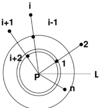
Figure 2: Step 1 of Graham’s algorithm. Midpoints of collinear points are deleted in an attempt to con-struct a point P that is within the interior of 3 non-collinear points ∈ S. 1 L P n 2 i-1 i i+1 i+2

Figure 3: Step 4 of Graham’s algorithm. Remove those points that lie on the same radial arm that are not maximally distant.

mension, and then constructing a centroid for those two ex-treme points. If they are the same, then all of the points are collinear, and the convex hull collapses to a line. ii) the po-lar transformations are straightforward and take O(n) iii) the θ sort will take nlog n

log 2 using the sorting routine

refer-enced in the paper. This can easily be seen to be O(n log n) iv) the deletion of close points, see Fig.3 requires O(n), and v) scanning and deleting points has two cases, as explicated in Fig.4. The total running time of Graham’s algorithm is: T(n) = O(n log n).

3.

JARVIS 1973

The general idea of the algorithm, is to first select a point outside of the input set S, and then construct one hull boundary segment at a time, in a counter clockwise man-ner. Fig.5 demonstrates how the angle θ, with respect to a horizontal line, could be calculated from an initial point pout

outside the bounding box of S. The minimum angle would be selected, and that endpoint would become the first point of the convex hull. In which case, the second step performs similarly to the first, but with the origin of the compar-isons emanating from the first convex hull point Fig.6. The procedure is repeated, from each of the points, with the

P

i

i+1

i+2

Case 1:

Case 2:

P

i

i+1

i+2

Figure 4: Two cases to consider in Graham’s algo-rithm. Either i) θ > π, in which case point i may be deleted, or ii) θ ≤ π, in which case point i becomes part of the hull and the next group of 3 points are considered by sliding forward by 1.

additional optimization that interior points of the hull un-der current construction no longer need to be consiun-dered Fig.7. The author [4] mentions an additional optimization in that the angle (θ) calculations may be substituted by sign tests (based on being located in one of the four quadrants). Jarvis’ algorithm [4] has a running time of T (n) = O(nm).

Jarvis_{(point set S ⊆ R}2₎ 1 Point pout← Outside(S )

2 Point pcurr ← pout

3 for each point pi∈ S

4 do 5 if pcurr6= pout 6 then 7 DelCheck(S) 8 θi← Angle(pcurr, pi) 9 pcurr← MinAngle() 10 CH(S) ← S

4.

CHAN 1995

Chan [1] uses the concept of running algorithm Chan() for a small value of H. If this fails, (poor randomly par-titions sets) then the algorithm is stopped and restarted with a larger H value to a maximum of H = n, the num-ber of points (since H can be when all of the points are on the convex hull). This algorithmic technique is called doubling. The Chan(P, m, H) basically attempts to find a convex hull of length H or less, if one exists, by artifi-cially constructing some partitions of size at most m. These partitions are each run through a convex hull algorithm (say Graham’s scan) and convex hulls are created contain-ing those partition points Fig.9. The convex polygons are then used informally as a set of large points in a Graham

0 2 4 6 8 10 12 14 16 18 0 5 10 15 20 25 30 variable 2 variable 1 Data Points

Figure 5: Jarvis’ algorithm need to compare a point with all of the rest.

0 2 4 6 8 10 12 14 16 18 0 5 10 15 20 25 30 variable 2 variable 1 Data Points

Figure 6: Jarvis’ algorithm picks the minimum θ (angle). 0 2 4 6 8 10 12 14 16 18 0 5 10 15 20 25 30 variable 2 variable 1 Data Points

Figure 7: The second step in Jarvis’ algorithm re-quires n − 1 evaluations. 0 2 4 6 8 10 12 14 16 18 0 5 10 15 20 25 30 variable 2 variable 1 Data Points Deletion Region

Figure 8: The i-th step in Jarvis’ algorithm is able to delete those points inside the growing hull boundary.

0 2 4 6 8 10 12 14 16 18 0 5 10 15 20 25 30 variable 2 variable 1 Data Points Partition 1’s ConvexHull Partition 2’s ConvexHull Partition 3’s ConvexHull

Figure 9: Example of 3 convex hulls each con-structed by, for example, Graham’s algorithm, sur-rounding the points in each of the 3 partitions of S as constructed by Chan’s algorithm.

Scan type manner. If no convex hull is found, then in-complete is returned and the doubling technique is used to search further. There are ceil(n

m) possibly overlapping

con-vex polygons, where each has at most m vertices. It takes O(m log m) for Graham’s scan. The preprocessing time is O(n

m(m log m)) = O(n log m) with h wrapping steps each

costing O(n

mlog m). Therefore, the total time is O(n log m+

h(n

mlog m)) = O(n(1 + h

m) log m) according to [1].

Chan(P, m, H)

1 partition P into subsets P1,· · · , Pceil(n

m)each of size at most m

2 for i = 1, · · · , ceil(n

m) Do

compute CH(Pi) by Graham’s scan

3 p0← (0, −∞)

4 p1← the rightmost point of P

5 fork = 1, · · · , H Do 6 fori = 1, · · · , ceil(n

m) Do

7 compute the point qi∈ Pithat maximizes

8 ∠pk

−1pkqi(qi6= pk) by binSearch(pi)

9 pk+1← point q ∈ {q1,· · · , qceil₍n m)} maximizing ∠pk₋₁pkq

10 if pk₊₁= p₁ Then return the list < p₁,· · · , pk>

11 return incomplete

ChanWrapper(P ) 1 for t = 1, 2 · · · ) Do

2 L← Chan(P, m, H), where m = H = min(22t , n) 3 if L 6= incomplete then return L

5.

CONCLUSIONS

Three planar convex hull algorithms have been explicated, along with their order of complexity in terms of their number of basic operations. Diagramatic descriptions of the correct-ness of each algorithm have also been presented. Within the time constraints imposed, a c-degree of depth of understand-ing has occurred, for some slightly large constant c.

Pk

Point On Hull

Pk-1

Pk+1

Figure 10: Find a point maximizing θ for a polygon, and choose the one maximizing θ over all polygons.

6.

ACKNOWLEDGMENTS

The author would like to thank Prof. Maheshwari for teach-ing the course. NRC-IIT-IR group for supportteach-ing my atten-dance at this course, in particular, the following people from NRC: Julio J. Vald´es, Bob Orchard and Fazel Famili. CISTI for supplying research materials. Professor Morin’s CH2() program. Implementors of the unix banner command.

7.

REFERENCES

[1] T. Chan. Optimal output-sensitive convex hull algorithms in two and three dimensions. In Discrete and Computational Geometry, volume 16, pages 361–368, 1996.

[2] T. M.-Y. Chan. Output-sensitive Construction of Convex Hulls. PhD thesis, University of British Columbia, October 1995.

[3] R. Graham. An efficient algorith[sic] for determining the convex hull of a finite planar set. Information Processing Letters, 1:132–133, 1972.

[4] R. Jarvis. On the identification of the convex hull of a finite set of points in the plane. Information Processing Letters, 2:18–21, 1973.

[5] L. C. Kinsey. Topology of Surfaces. Number ISBN 0-387-94102-9. Springer-Verlag, New York, 1993. [6] J. W. Tukey. Exploratory Data Analysis. 1977. [7] http://biogeometry.cs.duke.edu/software/

alphashapes/index.html. Alpha shapes introduction. October 31 2005.

[8] J. J. Vald´es and A. J. Barton. Relevant attribute discovery in high dimensional data based on rough sets applications to leukemia gene expressions. In Lecture Notes in Computer Sciences / Lecture Notes in Artificial Intelligence, Regina, Saskatchewan, September 1 2005.

[9] E. W. Weisstein. Polar coordinates. From MathWorld – A Wolfram Web Resource. http:

//mathworld.wolfram.com/PolarCoordinates.html, October 31 2005.