Publisher’s version / Version de l'éditeur:
Vous avez des questions? Nous pouvons vous aider. Pour communiquer directement avec un auteur, consultez la
première page de la revue dans laquelle son article a été publié afin de trouver ses coordonnées. Si vous n’arrivez
Questions? Contact the NRC Publications Archive team at
[email protected]. If you wish to email the authors directly, please see the first page of the publication for their contact information.
https://publications-cnrc.canada.ca/fra/droits
L’accès à ce site Web et l’utilisation de son contenu sont assujettis aux conditions présentées dans le site
LISEZ CES CONDITIONS ATTENTIVEMENT AVANT D’UTILISER CE SITE WEB.
Research Report (National Research Council of Canada. Institute for Research in Construction), 2005-03-01
READ THESE TERMS AND CONDITIONS CAREFULLY BEFORE USING THIS WEBSITE. https://nrc-publications.canada.ca/eng/copyright
NRC Publications Archive Record / Notice des Archives des publications du CNRC :
https://nrc-publications.canada.ca/eng/view/object/?id=651d4579-53fb-44a9-88f6-afd87935ce29 https://publications-cnrc.canada.ca/fra/voir/objet/?id=651d4579-53fb-44a9-88f6-afd87935ce29
Archives des publications du CNRC
For the publisher’s version, please access the DOI link below./ Pour consulter la version de l’éditeur, utilisez le lien DOI ci-dessous.
https://doi.org/10.4224/20374276
Access and use of this website and the material on it are subject to the Terms and Conditions set forth at
Material Emission Data - Small Environmental Chamber Tests. Phase 1, Materials Re-Analysis. Phase II, New Materials Tests: Final Report 3.1
Material Emission Data - Small
Environmental Chamber Tests.
Phase 1, Materials Re-Analysis.
Phase II, New Materials Tests :
Final Report 3.1
Magee, R.J.; Yang, W.; Won, D.Y.; Lusztyk, E.
IRC-RR-321
Material Emission Data -
Small Environmental Chamber Tests
Phase I Materials Re-Analysis
Phase II New Materials Tests
R. Magee, W. Yang, D. Won, E. Lusztyk
Final Report 3.1
CMEIAQ-II: Consortium for Material Emissions and IAQ Modelling II
Consortium for Material Emissions and Indoor Air Quality Modelling II (CMEIAQ-II)
In 2000, the Institute for Research in Construction, National Research Council Canada (IRC/NRC) launched the second phase of the Material Emissions and Indoor Air Quality Modelling project (CMEIAQ-II). The second phase of this project is the direct result of the support and suggestions from the first phase’s consortium members for continued work on this research topic. In the second phase, the research is directed towards two principal objectives. The first is to develop the knowledge and tools needed to estimate
concentrations of volatile organic compounds (VOCs) generated by the emissions from building materials and furnishings in order to gain a better understanding of the effects of those products on indoor air quality (IAQ). The second is to provide the scientific bases needed to enhance indoor air quality guidelines for office and residential buildings. An important addition to the project in this phase was the Health and End Users Advisory Committee, which was tasked to provide much needed input from the health sector and advice to help tailor the project outputs to better meet the needs of end-users.
Phase II Tasks
The specific tasks of the phase II research were:
• To assemble a target VOC list on which to focus our efforts for the analysis of
the emission test results. The list includes chemicals which are known to be emitted from various materials, and, especially, chemicals known to have health effects;
• To determine the ranges of variation of the emissions from selected materials,
which may result from material variability or environmental influences;
• To expand the database to include a total of 69 materials, and to re-analyze the
existing data to cover as many VOCs on the new target list as possible;
• To refine the Material Emission DataBase and Indoor Air Quality (MEDB-IAQ)
simulation program to make it more user-friendly;
• To develop and validate empirical and mass-transfer based source models; and
• To develop a best practice guide for managing VOCs/IAQ in office buildings.
Significance of the Project
A recent report by a multidisciplinary group of European scientists (EUROVEN) based on existing and limited literature, recommends that outdoor air supply rates need to be
increased to 30 L/s per person from the current ASHRAE recommendation of 10 L/s per person to improve indoor air quality for health, comfort, and productivity concerns. On the other hand, a previous NRC experimental study indicates that increasing the ventilation rate to speed up the removal of air-borne VOCs, even when energy use is not a concern, is not effective. The most efficient strategy to maintain indoor air quality is to remove the contaminants at the source (source control) and then to rely on ventilation (dilution) to remove the air-borne VOCs.
This research contributes to improve indoor air quality by developing knowledge and tools for effectively applying source control to reduce ventilation needs (and hence, save energy).
The work provides the relative contribution by a given product to up to 90 VOC concentrations (some of which are known to have adverse health effects), allowing
intelligent, informed choices of building materials and indoor consumer products. Product manufacturers will benefit by learning how their products can be improved with respect to VOC emissions, and where their products stand relative to others in simulations of their actual use. The information collected in Phase II will also make it easier for investigators to diagnose possible IAQ problems in buildings, and explore trade-offs between increased ventilation and source control.
The consortium for Phase II (which has a Steering Committee, a Technical Advisory Committee, and a Health & End Users Advisory Committee) was established to set the research priorities and help fund the project. Members of the consortium include: Public Works & Government Services Canada, Natural Resources Canada, Canada Mortgage and Housing Corporation, Health Canada and the National Research Council. In addition, the following organizations have made significant in-kind contributions to the consortium project through close research collaboration with the IRC/NRC project team: Canadian Composite Panel Association, Carleton University, Chemical Manufactures Association (Rohm & Haas), Dalhousie University, Gypsum Board Association, Saskatchewan Research Council, Syracuse University, University of Calgary, University of Miami, U.S. Environmental Protection Agency (EPA), U.S. National Institute of Standards and
Technology (NIST), and Virginia Polytechnic Institute & State University. The CMEIAQ-II final research reports include:
Report 1.1 Target VOC list
Report 1.2 Methodology for Analysis of VOCs in Emission Testing of Building
Materials
Report 2.1 Specimen Variability: A Case Study
Report 2.2 Effects of Environmental Factors on VOC Emissions from a Wet
Material
Report 2.3 Effects of Material Temperature on VOC Emissions from a Dry
Building Material
Report 3.1 Material Emission Data: Small Environmental Chamber Tests
Report 3.2 MEDB-IAQ Version 4.1 Beta
Report 4.1 Model Development for VOC Emissions from Wet Building
Materials
Report 4.2 Validation of a Mass-transfer Model for VOC Emissions from Wet
Building Materials
Report 4.3 Validation of Empirical Models with Long-term Emission Testing
Data
Report 5.1 Indoor Air Quality Guidelines and Standards
Report 5.2 Managing VOCs and Indoor Air Quality in Office Buildings: An
Reports 1.1 and 1.2 provide the information on the Target VOC list and the analysis method for the VOCs on the list. Reports 2.1 and 2.2 present research outcomes on both inherent and environmental factors inducing variability in material emissions. Report 2.3 discusses VOC emissions as a function of surface temperatures, which can be applied to emissions from a radiant floor heating system. Report 3.1 provides material emission testing data and the resulting coefficients for empirical emission models for the expansion of MEDB-IAQ simulation software. Report 3.2 is a user manual for the revised MEDB-IAQ. Reports 4.1 and 4.2 deal with the development of a mass-transfer based model for wet building
materials and the validation of the model with experimental data. Report 4.3 compares empirical models based on short-term emission testing data with those based on long-term data. Report 5.1 contains summaries of existing guidelines and standards associated with indoor air quality. Report 5.2 is a manual for property managers and building operators for their duties in managing VOCs in office buildings.
Table of Contents:
List of Figures: ... vi
List of Tables: ... vi
1. Introduction ... 1
2. Methodology of Emission Testing and Data Analysis ... 1
2.1 Re-analysis of Phase I tests ... 1
2.2 Phase II Tests ... 2
2.2.1 Selection of Candidate Building Materials ... 2
2.2.2 Experimental Procedures ... 2
2.2.2.1 Specimen descriptions, handling, and preparation ... 2
2.2.2.1.1 Laminate Flooring and Laminate Flooring Assembly (Lam1, 2, 3) . 2 2.2.2.1.2 Linoleum and Linoleum Assembly (Lin1, 2) ... 4
2.2.2.1.3 Hardwood Flooring (HWF1) ... 5
2.2.2.1.4 Medium Density Fiberboard (MDF1, 2, 2b) ... 5
2.2.2.1.5 Kitchen Countertop (CT1, 2) ... 6
2.2.2.1.6 Carpet and Carpet Assembly (Crp7, 7a) ... 6
2.2.2.1.7 Vinyl-Faced Gypsum Panel (VWB1) ... 7
2.2.2.1.8 Oriented Strand Board (Variability and Long-Term Emissions Tests OSB4; OSB5a,b,c,d; OSB6a,b; OSB7a,b) ... 7
2.2.2.1.9 Oil-Based Wood Stain (WS6a and WS6b) ... 7
2.2.2.2 Chamber Testing ... 7
2.2.2.3 Chemical Sampling and Analysis ... 8
2.2.2.3.1 GC/MS ... 8
2.2.2.3.2 HPLC ... 8
2.3 Methodology of Empirical Modelling ... 10
2.3.1 Method to Estimate Emission Factors ... 10
2.3.2 Empirical Modelling Procedures and Criteria ... 12
2.3.2.1 Regression Process... 12
2.3.2.2 Quality Improvement Process ... 13
2.3.2.3 Model Selection Process ... 14
3. Results and Discussion of Emission Testing and Empirical Modelling ... 17
3.1 VOC Emissions: Re-Analysis of Phase I Data ... 17
3.2 VOC Emissions: Phase II New Materials ... 19
3.2.1 Laminate Flooring and Laminate Flooring Assembly ... 21
3.2.2 Linoleum and Linoleum Assembly ... 23
3.2.3 Hardwood Flooring ... 24
3.2.4 Medium Density Fiberboard ... 25
3.2.6 Carpet and Carpet Assembly ... 27
3.2.7 Vinyl-Faced Gypsum Panel ... 28
3.3 Empirical Modelling ... 29
4. References ... 31
Appendix 1 – Measured Concentrations of Target VOCs in Chamber Air for Materials
Tested in CMEIAQ-I A1-1
Appendix 2 – Coefficients of Empirical Models of Target VOCs in Chamber Air for
Materials Tested in CMEIAQ-I A2-1
List of Figures:
Figure 1: An example case with improved R2 by recalculating the deviated data points . 13
Figure 2: An example case with improved R2 by removing the deviated data point... 13
Figure 3: An example case with improved R2 by removing the first low EF value ... 14
Figure 4: An example case with improved R2 by removing the first highest EF value .... 14
Figure 5: An example case where a Peak Model was selected for its substantially better R2 value ... 15
Figure 6: A example case where a Peak model was selected for its better performance in long-term predictions ... 15
Figure 7: Example cases where the models on the right-hand side were selected for their better long-term prediction performance ... 16
Figure 8: VOCs present in 24h samples from Phase I tests. ... 18
Figure 9: VOCs present in 24h samples from Phase II tests ... 20
Figure 10: VOC profile for Laminate flooring tests. ... 21
Figure 11: Formaldehyde emission from Tests Lam1, 2, and 3. ... 22
Figure 12: VOC profile for Linoleum flooring tests. ... 23
Figure 13: VOC profile for Prefinished Hardwood Oak flooring test. ... 24
Figure 14: VOC profile for Medium Density Fibreboard test. ... 25
Figure 15: VOC profile for Countertop tests. ... 26
Figure 16: VOC profile for Carpet tests. ... 27
Figure 17: VOC profile for Vinyl-faced Gypsum Panel test. ... 28
List of Tables: Table 1: Test materials – Phases I and II. ... 3
Table 2: Target VOC List. ... 9
Table 3: Carbonyl compounds analyzed by HPLC... 10
Table 4: Percentage (%) of models with R2 greater than 0.7 for materials tested in Phase I of CMEIAQ ... 29
Table 5: Percentage (%) of models with R2 greater than 0.7 for materials tested in Phase II of CMEIAQ ... 29
Table 6: Percentage (%) of models with R2 greater than 0.7 for each group of target VOCs: ... 31
1. Introduction
One of the objectives of the Phase II Consortium on Material Emissions and Indoor Air Quality was to expand the database of building materials emissions generated in Phase I. This was accomplished in two ways.
In Phase I, while identification of emitted VOCs from the 24-hour sample was extensive, detailed investigation of the emissions profiles of individual VOCs was limited to 3-5 VOCs per material. The development of a target list of 90 VOCs in Phase II, with the input and approval of the Health and End-User Advisory Committee, provided the basis for re-examination of the Phase I results (refer to Phase II Report 1.1 for a complete explanation of the target list and its development). This re-examination was possible for 43 of the original 48 Phase I tests (several of the earliest tests having been analyzed exclusively by GC/FID or by an earlier model of GC/MS from which the data format did not permit re-analysis). The results of the 90 target compound re-analysis of these 43 Phase I tests is reported here.
Secondly, with input from the Phase II Technical Advisory Committee, a new series of building material emissions tests were conducted. The TAC expressed its desire to expand our knowledge related to the emissions characteristics of material assemblies. In response, the new tests included single material emission investigations of seven new building materials (linoleum flooring, laminate flooring, carpet, pre-finished hardwood flooring, vinyl-faced gypsum panel, medium density fibreboard, and a countertop
material); plus four tests with assemblies of these materials (linoleum/adhesive/plywood; laminate/underlay; laminate/underlay/OSB; and carpet/adhesive/concrete). “Headspace” analyses of VOCs were also conducted for the underlay material, the two adhesives, the plywood, and the concrete substrate for the carpet assembly. Separate tests were
conducted with the countertop material in which all surfaces and only the upper laminate surface were exposed in the emissions chamber. The results of the emission trials for these new materials, and their assemblies, compared against the 90-compound target list, are presented here.
2. Methodology of Emission Testing and Data Analysis
The procedures reported here relate to a) the re-analysis of the Phase I emissions tests and b) the experimental protocols associated with the procurement, handling, testing and analysis of the new Phase II materials and assemblies of materials. Where appropriate, reference is made to earlier, detailed reports of these methods.
2.1 Re-analysis of Phase I tests
Of the 48 original Phase I tests, only 5 could not be re-analysed for emissions of the 90 VOCs listed in the target list. These tests were: PB4,5,6 (particleboard) and WS2,9 (woodstain). The GC/MS data from remaining 43 tests were re-examined according to the methodology outlined in Phase II Report 1.2. Tables of the concentration of all 90 target VOCs vs. time for each test were generated. Empirical modelling of the data was
subsequently conducted (power law model for dry materials, segmented VB plus power law model for the wet materials). The model coefficients and their correlation will be reported. The Material Emissions Database and Indoor Air Quality simulation program (MEDBIAQ) will be updated with these new coefficients.
2.2 Phase II Tests
2.2.1 Selection of Candidate Building Materials
With input from CMEIAQ-II’s TAC, a list of candidate building materials and assemblies was determined. In total, approximately 30 materials of interest were identified. The TAC members were then asked to vote on their preferences. A final list of materials was circulated for approval by the TAC members. The building materials selected for Phase II are listed in Table 1, together with those tested in Phase I.
Reflecting the interests of the Consortium members, Phase II material selection struck a balance between commercial and residential products, and material assembly testing was emphasized.
2.2.2 Experimental Procedures
The general test procedures and analytical methodology employed in this study have been previously described in CMEIAQ-I Final Reports 1.2 (Sampling and Analysis of VOCs) and 1.2 (Test Method – VOC Emissions from Dry Building Materials). CMEIAQ-II Final Report 1.2 (VOC Analysis – Building Materials) describes the refinements
developed in the analytical methodology that were applied to the Phase II tests and the re-analysis of the Phase I data. Where comparisons between emissions from single products with that from assemblies of materials were to be made, tests were conducted
simultaneously using specimens taken as close to one another from the original product sample in an effort to eliminate any effect due to the age of the specimens, and, as much as possible, any specimen inhomogeneity.
2.2.2.1 Specimen descriptions, handling, and preparation
2.2.2.1.1 Laminate Flooring and Laminate Flooring Assembly (Lam1, 2, 3)
Laminate flooring is an increasingly popular flooring material that is produced by a diverse spectrum of manufacturers/brands (one web-site alone lists 38 separate manufacturers, many with multiple product lines of this material). Several building material suppliers in the Ottawa region were canvassed to note local availability. The selected material was chosen in part due to its claim to be a “Green” “wood-free” material (manufactured from agricultural residues). The product was a glueless “snap” variety, reflecting the trend away from glued laminate flooring. An intact sealed box (plastic wrapped) of the flooring was purchased together with a bundle of the foam underlayment recommended by the retailer as being typically installed with this material (this also sealed in a plastic bag). The laminate and underlay were immediately returned to the lab, cut and transferred to clean specimen bags per the test protocol. The laminate
Table 1: Test materials – Phases I and II.
Category Phase I (48 tests) Phase II (21 tests)
Solid and Engineered Wood Materials
Plywoods (3) G1S Fir, 19.1mm
Spruce Sheathing, 12.7 & 15.9mm
Medium Density Fibreboard
15.9 mm
Oriented Strand Boards (3) 11.1mm O-2
12.7mm R-1
15.9mm O-2 Oriented Strand Boards 14.5mm, T&G Subfloor (9)
o Specimen Variability Tests (9), including
o 2-Long-Term Tests
Solid Woods (3)
Oak (strip flooring, unfinished) Pine
Maple
Particleboards (3)
15.9mm industrial (3 separate mills)
Installation Materials
Caulking/Sealants (3) Silicon
Polyurethane
Thermoplastic (see below for Adhesives tested with
Linoleum and Carpet Assemblies)
Adhesives (3) Form Board Construction “VOC-Free” Flooring Materials Vinyl Floors (3)
Tile (1 Residential; 1 Commercial) Sheet (Residential)
Hardwood Floor (Oak, Pre-Finished)
Linoleum Floor Tile, 2.5mm
Assembly: Linoleum / Adhesive /
Plywood Underpads (3)
Polyurethane Foam Urethane Foam Chip Polyethylene Foam
Laminate Floor (wood-free, 6mm, glueless)
Assembly: Laminate / Underlay Assembly: Laminate / Underlay / OSB
Carpets (6) Residential (3)
o Nylon/Latex (3 different manufs) Commercial (3) o Olefin o Polypropylene o Nylon Carpet Nylon/Latex (Commercial)
Assembly: Carpet / Adhesive / Concrete
Interior Wall Panels Gypsum Panels (3) Standard Fire-Code Water Resistant
Vinyl-Faced Gypsum Wall Panel
Ceilings
Acoustical Ceiling Tiles (3) Perlite (commercial)
Vinyl-coated fiberglass (commercial) Cellulose (residential)
Table 1 (continued): Test materials – Phases I and II.
Category Phase I (48 tests) Phase II (21 tests)
Interior Finishes Paints (3) Latex Primer Latex Interior Alkyd Interior Floor Waxes (3) Paste, oil-based (2) Liquid, water-based Woodstains, oil-based (3) Polyurethanes, oil-based (3) 1 clear, 2 semi-gloss Interior Furnishings Countertop (Melamine/particleboard core): 2 tests of same material:
upper laminated surface only
all surfaces exposed (incl. Melamine iron-on end trim)
was cut such that two pieces would be connected, forming a longitudinal joint exposed in the sample holder. Three separate tests laminate flooring tests were conducted. The first, “Lam1” tested an assembly of the laminate and foam mounted in the specimen holder (upper surface of laminate floor as sole exposed surface). A fresh box of the laminate was purchased from the retailer (same production batch) for use for the remaining 2 tests, which were conducted simultaneously in separate chambers. A piece of OSB was also purchased at this time (subject to the same collection and handling procedures as used for OSB specimens 4 through 7). “Lam2” tested the laminate alone, while “Lam3” tested an assembly of laminate + underlay + OSB. In all cases, only the upper surface of the laminate floor was exposed through the use of specimen holders. A piece of the foam underlay was “headspace” evaluated via conditioning in a clean sampling bag flushed
with ultra zero grade air and left for 24 hours at 23oC. The OSB used for this test was a
fresh specimen of the same product that had been previously tested (OSB4 through 7). Its emission characteristics have been described in detail in Phase II Report 2.1.
2.2.2.1.2 Linoleum and Linoleum Assembly (Lin1, 2)
Linoleum flooring was one of the building materials recommended for evaluation by the CMHC member of the technical advisory committee. On further consultation with that member, the product line tested was selected as being representative of residential installations. A box of 2.5mm thick tiles was ordered through a local flooring company, as was the recommended adhesive for its installation. The adhesive (manufactured by the same company as the linoleum tile) was rated as having “low solvent content”. An alternative adhesive was also available, marketed as a “Green” product and “Solvent-free, extremely low emission”, but the adhesive recommended by the supplier as that which was typically used was selected. Two tests were conducted: “Lin1” tested the emission from the upper surface of the tile alone, while “Lin2” tested an assembly of linoleum tile glued onto plywood underlay (1/4” thick, purchased from local retailer). The trowel recommended by the adhesive manufacturer for this application was purchased and
employed for preparation of the material assembly. The tile was pressed onto the
plywood/adhesive using a clean metal tube to simulate the recommended rolling pressure for the product. After weighing of the assembly (to determine mass of adhesive applied) the test specimen was immediately placed in the holder and then into the test chamber. The time lag from application of the adhesive, to sealing of the holder-mounted specimen within the chamber was 9 minutes. A portion of the adhesive was also placed in a clean petri dish and sealed in a clean sample bag, flushed 3 times with ultra zero quality
compressed air, and then left in a temperature controlled room (23 oC +/- 0.5 oC) for 24
hours. A sample of the plywood underlay was similarly treated. Headspace air samples were collected from these samples after 24 hours and analyzed by GC/MS to identify VOCs emitted by these assembly components.
2.2.2.1.3 Hardwood Flooring (HWF1)
Hardwood flooring is re-gaining favour as a residential finishing material. Pre-finished flooring strips appear to dominate this market. Un-finished oak flooring strips were tested in Phase I as part of the series of wood products. As an extension to this effort, pre-finished oak was selected this time to better evaluate the impact of the finish coating. The 3-1/4 x 3/4" strips were purchased from a local retail outlet in an unopened, plastic wrapped box. Grade was “Select and Better”. The Satin – Aluminum oxide finish was claimed by the manufacturer to be an “above average varnish thickness". Two pieces of the flooring were cut such that on assembly (press fit), a longitudinal joint remained exposed in the sample holder. The power blackout that hit eastern North America in Aug. 2003 brought a sudden termination to test “HWF1”. Although the backup power system developed for the test chamber air supply/control system successfully maintained chamber operation during this event, the test was terminated when the chamber
temperature began to rise due to the lose of the laboratory’s air conditioning. Analysis of the air samples from the shortened test indicated that sufficient samples had been
collected to characterize the extremely low emissions from this product, and the decision was made, therefore, not to repeat the test.
2.2.2.1.4 Medium Density Fiberboard (MDF1, 2, 2b)
Medium density fibreboard, or “MDF”, is being employed in a widening range of applications in construction. Originally used as a trim material or cabinet backing, it is moving into structural applications as formulation/processing advancements enable production of increasingly thicker panels made from this class of material. As a compromise to the range of available MDF products, 5/8” thick shelving panels were purchased from a local retailer. The initial test of this material, “MDF1” was
compromised when a failure of the air conditioning system for the environmental
chamber occurred about 54 hours into the test, resulting in test temperatures of 27 oC
lasting approximately 25 hours. The specimen remained in the chamber during this period, and sampling was continued for an additional 5 days following temperature restoration, but the test was repeated (as “MDF2”) with a freshly obtained specimen. To further examine the impact of specimen conditioning on VOC emissions, specimen “MDF2” was transferred after 11 days to a second chamber and re-commenced as test “MDF2b”. The results of these temperature impact and conditioning evaluations will be reported separately.
2.2.2.1.5 Kitchen Countertop (CT1, 2)
As with laminate flooring, a wide range of countertop materials is available (typically for the residential market, although not exclusively). For standard residential
construction/renovation, a laminate surface over a particleboard core is the dominant product. Several retail outlets were canvassed to identify common countertops products. The unit that was selected was purchased in a five-foot length together with the end trim application kit supplied by the manufacturer. The data of production of the countertop was stamped on the bottom surface. Two sections of the countertop were cut from the center of the specimen to fit the standard specimen holders. End trim was applied to one edge only of each cut specimen, to approximate the portion that would be covered in a typical installation. The two specimens were tested simultaneously in separate chambers. The first specimen, CT1, was mounted normally in its specimen holder such that only the top laminated surface was exposed to the chamber air. The second specimen, CT2, while also placed in a holder for consistency, was mounted low in the holder, such that the holder’s top plate did not form a seal with the laminate surface. Additionally, small inert shims were placed under the specimen, so that the bottom surface was also freely
exposed. As a result of this mounting procedure, all surfaces (top laminate, edge with laminate trim, and 3 edges and bottom surface of exposed particleboard) were exposed to the chamber.
2.2.2.1.6 Carpet and Carpet Assembly (Crp7, 7a)
In an attempt to obtain a commercial carpet specimen that would be typical of current renovation practices, the Properties and Facilities Management Group of Public Works and Government Services Canada (PWGSC) was contacted for assistance. Their prompt and timely help in supplying both a carpet specimen and a container of the adhesive used in its application at an active renovation in a Federal building in the National Capital Region is gratefully acknowledged. Special thanks doe DG Sue Hum-Hartley and to Wilf Leblanc, Head of Special Projects Group for their help.
The carpet supplied was a nylon fabric with a latex backing that had recently been delivered to the renovation site. The “non rigid” adhesive was also delivered directly from the renovation site. Two tests were conducted simultaneously. The first, Crp7 (extension of the six carpet samples tested in Phase I), was a carpet only test. The second, Crp7a, was an assembly of this carpet, glued to a concrete substrate with the supplied adhesive. The concrete was cut to fit the specimen holder from one of several slabs prepared for use in earlier investigations of glue-down carpet emissions that had been stored in the basement of building M24. The slab was removed from the centre of the stack and cut using a water-flushed masonry saw in the lab. The slab was conditioned for several days at 50% RH (1 ACH) in one of our chambers prior to testing. A
“headspace” sample from the chamber was collected to characterize any emissions coming from the concrete itself. The adhesive was applied to the concrete using the trowel recommended by the instructions printed on the adhesive container. The time lag between application of the adhesive to the concrete and the sealing of the carpet/
2.2.2.1.7 Vinyl-Faced Gypsum Panel (VWB1)
The procurement protocol that was used for the carpet specimen was also applied with the specimen of vinyl-faced gypsum panel. Pre-finished panels are commonly used in commercial construction. As with the carpet test, collection of a representative specimen was sought through attainment of the material from an active renovation site. This was accomplished through PWGSCs timely help, and their assistance is gratefully
acknowledged.
2.2.2.1.8 Oriented Strand Board (Variability and Long-Term Emissions Tests OSB4; OSB5a,b,c,d; OSB6a,b; OSB7a,b)
To meet the Phase 2 objectives of determining a) the impact of specimen variability on VOC emissions, and b) the reliability of using short-term test data to predict long-term emissions behavior, a series of new tests were conducted with OSB specimens (9 tests in all), all with a single type (grade, thickness, and application) of OSB produced at the same mill and purchased at the same retail outlet. A detailed description of the test methodology and results of the variability trials is given in Report 2.1, while the long-term emissions test results are the subject of Report 4.3. The experimental conditions, raw data and modeled emission coefficients for these 9 tests are reported here.
2.2.2.1.9 Oil-Based Wood Stain (WS6a and WS6b)
In Phase 1, results were given for the emissions from 3 separate wood stains applied to a maple substrate. An additional test, not reported in Phase 1, was also conducted with one of the stains applied to an oak substrate. The impact of substrate on emissions from the stain was thus investigated. Results for the two tests of this stain (on oak and maple) are reported here as tests WS6a and WS6b, respectively.
2.2.2.2 Chamber Testing
The emissions testing protocol employed was in accordance with guidelines specified by ASTM D5116 (1997) and has been previously described (CMEIAQ Phase I Report 1.2).
In summary, the rectangular 0.05 m3 environmental test chambers were constructed from
stainless steel (SS) with inner dimensions of 0.50 m (W) by 0.25 m (H) by 0.40 m (D). All inner surfaces were electro-polished. Clean air, generated by an Aadco molecular sieve filtration system with methane reactor and conditioned to 50% relative humidity by a mass flow controller-based system connected to impingers filled with HPLC-grade water, entered the chamber through an inlet manifold. Exhaust air exited through a manifold on the opposite side of the chamber. Sampling ports on the exhaust air line were used for sample collection. Temperature and humidity probes mounted in both the inlet and exhaust air streams continuously monitored chamber conditions and were the basis for environmental control. A pressure sensor connected to the chamber
continuously monitored the differential pressure. The chambers were placed in a temperature-controlled environment and were operated at 23 ± 0.5°C temperature, 50 ± 2% relative humidity and 1 air change per hour (0.833 L/min). Air mixing in the
chambers was confirmed using a tracer gas technique. The air leakage rate at a chamber pressure of 10 Pa was less than 3%. The average surface velocity over the sample specimen was < 0.05 m/s.
2.2.2.3 Chemical Sampling and Analysis
A detailed description of the VOC sampling and analysis procedures can be found in CMEIAQ-II Report 1.2. A brief summary is given below.
2.2.2.3.1 GC/MS
Supelco Carbotrap 300 tubes were used for air sampling. These three-bed tubes were designed to maximize the collection of VOCs in a wide range of volatility. The volume of the sample, depending on the concentration of the VOCs, was from 10 mL to 15 L with a sampling rate not higher than 200 mL/min. VOC analysis was performed using a Perkin-Elmer ATD400 thermodesorber connected with Gas Chromatography/Mass Spectrometry Agilent MSD 5973. For detailed discussion of calibration and analysis procedures, refer to CMEIAQ-II Report 1.2.
The 90 VOCs included in the Target List are shown in Table 2. Refer to CMEIAQ-II Report 1.1 for a detailed explanation of the derivation of this list.
2.2.2.3.2 HPLC
HPLC analysis of carbonyl compounds in the chamber exhaust air was performed in accordance with ASTM D5197 and EPA TO-11. Exhaust air from the test chamber was pumped through a SPE cartridge (Waters Sep-Pak XpoSure Aldehyde) coated with DNPH (2, 4-dinitrophenylhydrazine). The cartridge was washed with acetonitrile, and the eluate analyzed by isocratic reverse phase HPLC with UV detection at 360nm (Varian Model 9012 Solvent Delivery System/ 9050 Variable Wavelength UV-VIS Detector /
Prostar 410 Autosampler; two Supelcosil LC-18 columns (25cm x 4.6mm, 5μm) in series
at 300C). A gradient of acetonitrile in water from 60% to 100% were used for separation
of the carbonyl compounds. System calibration was performed using a six-point
calibration from a commercial DNPH derivative mixture (TO-11/IP-6A Aldehyde/Ketone reference standard from Supelco, Inc). The carbonyl compounds analyzed with HPLC are shown in Table 3.
Table 2: Target VOC List.
# /90
VOC
Class CAS # VOC
# /90
VOC
Class CAS # VOC
1 A ld e h y d e s 75-07-0 Acetaldehyde 54 A ro m a ti c H y d ro c a rb o n s 95-93-2 1,2,4,5-Tetramethylbenzene 2 107-02-8 Acrolein 55 611-14-3 2-Ethyltoluene 3 100-52-7 Benzaldehyde 56 620-14-4 3-Ethyltoluene 4 123-72-8 Butanal 57 622-96-8 4-Ethyltoluene 5 112-31-2 Decanal 58 4994-16-5 4-Phenylcyclohexene 6 50-00-0 Formaldehyde 59 71-43-2 Benzene 7 98-01-1 Furfural 60 526-73-8 1,2,3-Trimethylbenzene 8 111-71-7 Heptanal 61 95-63-6 1,2,4-Trimethylbenzene 9 66-25-1 Hexanal 62 95-47-6 1,2-Dimethylbenzene 10 124-19-6 Nonanal 63 108-67-8 1,3,5-Trimethylbenzene 11 124-13-0 Octanal 64 108-38-3 1,3-Dimethylbenzene 12 110-62-3 Pentanal 65 106-42-3 1,4-Dimethylbenzene 13 K et o n es
78-93-3 Methyl ethyl ketone 66 98-82-8 Isopropylbenzene
14 67-64-1 Acetone 67 103-65-1 Propylbenzene
15 98-86-2 Acetophenone 68 100-41-4 Ethylbenzene
16 108-94-1 Cyclohexanone 69 91-20-3 Naphthalene
17 108-10-1 Methyl isobutyl ketone 70 99-87-6 Isopropyltoluene 18 A lc o h o ls , Gl y c o ls , G ly c o E th e rs 107-21-1 1,2-Ethanediol 71 100-42-5 Styrene 19 4254-15-3 1,2-Propanediol 72 108-88-3 Toluene 20 71-36-3 1-Butanol 73 C ycl o A lk an es 110-82-7 Cyclohexane 21 107-98-2 1-Methoxy-2-propanol 74 1678-93-9 Butylcyclohexane 22 71-23-8 1-Propanol 75 1678-91-7 Ethylcyclohexane 23 111-76-2 2-Butoxyethanol 76 1678-92-8 Propylcyclohexane 24 112-34-5 2-Butoxyethoxyethanol 77 493-02-7 Decahydronaphthalene 25 110-80-5 2-Ethoxyethanol 78 T er p en es 80-56-8 alpha-Pinene 26 104-76-7 2-Ethyl-1-hexanol 79 99-86-5 alpha-Terpinene 27 109-86-4 2-Methoxyethanol 80 127-91-3 beta-Pinene 28 75-65-0 2-Methyl-2-propanol 81 99-85-4 gamma-Terpinene 29 67-63-0 2-Propanol 82 13466-78-9 3-Carene 30 64-17-5 Ethanol 83 79-92-5 Camphene 31 108-95-2 Phenol 84 5989-27-5 Limonene 32 E st er s 108-21-4 1-Methylethyl acetate 85 O th e r 3777-69-3 2-Pentylfuran 33 111-15-9 2-Ethoxyethyl acetate 86 872-50-4 1-Methyl-2-pyrrolidinone
34 123-86-4 Butyl acetate 87 64-19-7 Acetic acid
35 141-78-6 Ethyl acetate 88 142-62-1 Hexanoic acid
36 6846-50-0 TM-PD-DIB** 89 142-96-1 n-Butyl ether
37 H al o C a rbo
ns 95-50-1 1,2-Dichlorobenzene 90 109-52-4 Pentanoic Acid
38 106-46-7 1,4-Dichlorobenzene
39 75-09-2 Methylene chloride Notes:
40 79-01-6 Trichloroethylene ** TM-PD-DIB = 2,2,4-Trimethyl-1,3-Pentanediol Diisobutyrate 41 A li p h a ti c H y d d ro c a rb o n s 107-83-5 2-Methylpentane 42 96-14-0 3-Methylpentane 43 124-18-5 Decane 44 112-40-3 Dodecane 45 142-82-5 Heptane 46 544-76-3 Hexadecane 47 110-54-3 Hexane 48 111-84-2 Nonane 49 111-65-9 Octane 50 629-62-9 Pentadecane 51 629-59-4 Tetradecane 52 629-50-5 Tridecane 53 1120-21-4 Undecane
Table 3: Carbonyl compounds analyzed by HPLC.
No. CAS # Compound Class
1 50-00-0 Formaldehyde* ALD 2 75-07-0 Acetaldehyde* ALD 3 107-02-8 Acrolein* ALD 4 67-64-1 Acetone KET 5 123-72-8 Butanal ALD 6 100-52-7 Benzaldehyde ALD 7 110-62-3 Pentanal ALD 8 66-25-1 Hexanal ALD
• Compounds quantified exclusively by HPLC
2.3 Methodology of Empirical Modelling 2.3.1 Method to Estimate Emission Factors
This section explains the method of calculating emission factors based on chamber air concentration data. The emission factors will be used to estimate best-fit coefficients of empirical emission models through curve fitting.
The mass balance for the chamber can be expressed by Equation 1:
A EF C Q C Q t d C d V = in− + (1)
where C: Air concentration in the chamber (mg/m3)
V: Chamber volume (m3)
Q: Airflow rate (m3/h).
A: Surface area (m2)
EF: Emission factor (mg/m2/h)
Assuming Cin = 0, Equation 1 can be simplified:
L NC t C EFm + ∆ ∆ = (2)
where EFm: Emission factor calculated based on measured concentrations (mg/m2/h)
N: Chamber air change rate (1/h) as a ratio of Q and V. L: Material loading ratio (m2/m3) as a ratio of A and V.
Equation 1 is also recommended in ASTM Standard D5116 as a method to calculate emission factors when emission rate is not constant and/or the chamber has not reached steady-state (ASTM, 1997). When there are not enough data points available and the chamber has reached steady-state, Equation 2 can be simplified to Equation 3.
L NC
EFm = (3)
ASTM Standard D5116 recommends a method to calculate the slope of ∆C/∆t based on three data points. Since the method leads to n-1 emission factors from n+1 data points, a new method based on two data points was used to calculate the slope in this research (Equation 4). Although the new method saves only one more data point, it sometimes makes a difference when there are not many data points.
i i i i t t C C t C − = ∆ ∆ + − + 1 1 (4)
Therefore, a new set of concentration versus time data was also generated by Equations 5 and 6.
2 1 i i C C C= + + (5) 2 1 i i t t t = + + (6)
The following three equations (Equations 7, 8 and 9) were fitted to the calculated emission factor versus time data. In the Phase I project, the power-law model was recommended for emissions from dry building materials, while three segmented models were recommended for emissions from wet building materials. Since the segmented models tend to generate discontinuity in predicted concentrations, a peak model was introduced in this phase mainly for emissions from wet materials. However, the peak model was also chosen for dry materials when it’s necessary and vice versa for the power-low model. When there is not much change in the calculated emission factors, a constant model was used.
b p at EF = (7) − = 2 ln 5 . 0 exp b x t a EFp o (8) a EFp = (9)
where EFp: Emission factors predicted with empirical models (mg/m2/h)
a, b, xo: constants
2.3.2 Empirical Modelling Procedures and Criteria
The procedures of curve fitting and the criteria to select a particular model are explained in this section. Curve fitting was performed using SigmaPlot 2001 for Windows Version 7.0, which uses a non-linear regression method for a non-linear model. Microsoft Excel was not used for curve fitting in this research since it uses transformed regression model for logarithmic, power, and exponential trend lines. While transformation to a linear model has been used widely mainly for convenience, it can be used only when multiplicative errors are assumed (Equation 10)
i i
i t
Y =αexp(−β )ε
(10)
When additive errors (Equation 11) are assumed, the model cannot be linearized with any transformation and, hence, is intrinsically nonlinear (Rawlings, 1988).
i i
i t
Y =αexp(−β )+ε
(11)
In general, transformation of data to linear model is to be strongly discouraged because the errors on the transformed variables do not have a linear relationship to the errors on the observations (Gans, 1992).
The regression results (equation parameters and R2) and the time of first EF value (t1) are
reported in Appendix 2 for materials tested in Phase I and in Appendix 3 for materials tested in Phase II. It was assumed that EF value is constant before the time of the first
data point (t1). The R2 value is the coefficient of determination, which measures how
well a regression model describes the data. When R2 is close to 1, it indicates that the
resultant equation is a good description of the relation between the Emission Factor and the elapsed time.
The parameter of a constant model of Equation 9 was obtained by averaging Emission
Factors over a whole range of time. Therefore, no values of t1 and R2 were reported for a
constant model.
2.3.2.1 Regression Process
The empirical modelling procedure consists of three steps: regression process, model improvement process and model selection process.
The first regression process is composed of:
• Input the data of Emission Factor vs. elapsed time into SigmaPlot. • Choose the Statistics menu Regression Wizard command.
• Select an equation:
- For the Power-law model, choose a 2-Parameter equation (Equation 7). - For the Peak model, choose a Log Normal, 3-Parameter equation (Equation 8). • Adjust other equation settings and options, such as initial parameters, parameter constraints, and number of iterations or step size.
2.3.2.2 Quality Improvement Process
This regression process was then followed by a model improvement process:
• The R2
value of 0.7 was used as a criterion. If R2 was smaller than 0.7, data were
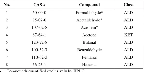
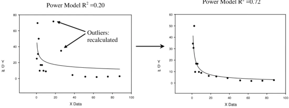
checked for outliers. If a data point was recognized as an outlier, the following steps were followed. If an average value of two concentration data was used to calculate an emission factor (EF), these concentration values were carefully examined. If possible, one single appropriate concentration value was selected to recalculate the EF value, instead of the average value used initially (Figure 1). In some cases, it was necessary to discard one or two data points that deviate considerably from the fitting curve (Figure 5). By recalculating the emission factor or, eventually, eliminating these outliers, and
recalculating the following EF values, we could significantly improve the regression results.
Figure 1: An example case with improved R2 by recalculating the deviated data points
Figure 2: An example case with improved R2 by removing the deviated data point 2D Graph 22D Graph 212D Graph 18
X Data 0 50 100 150 Y D at 0.2 0.4 0.6 0.8 1.0 1.2 1.4 1.6 Peak model R2=0.88 2D Graph 1322D Graph 61 2D Graph 29 X Data 0 50 100 150 Y D at 0.0 0.2 0.4 0.6 0.8 1.0 1.2 1.4 1.6 Peak model R2=0.19 Outliers: removed 2D Graph 2D Graph
Power Model R2 =0.20 Power Model R2 =0.72
X Data 0 20 40 60 80 100 Y D at 0 20 40 60 80 X Data 0 20 40 60 80 100 Y D at 0 10 20 30 40 50 60 Outliers: recalculated
• If R2
was small and there was no apparent presence of deviated data points, regression model was improved by removing the first one or two data points that were considerably lower (Figure 3) or higher (Figure 4) than the other data points.
Figure 3: An example case with improved R2 by removing the first low EF value
Figure 4: An example case with improved R2 by removing the first highest EF value
The first considerably lower or higher value was mostly caused by the sudden increasing or decreasing VOC concentration at the beginning of a test. In these cases, the regression models for both Power-law and Peak equations tend to be skewed towards the
dominating data points at the beginning, causing poor fitting performance for the
following tail-end data points. Removing these dominating data points to ensure a better prediction performance was a necessary step in this process.
2.3.2.3 Model Selection Process
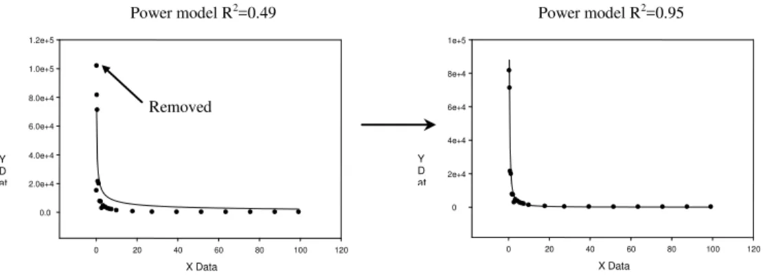
The last step is the model selection process:
Model selection favors the power-law model, since it has two coefficients to be
estimated. If the Peak model outperformed the Power-law model substantially (Figure 5),
2D Graph X 0 20 40 60 80 100 Y D at 0 20 40 60 80 100 120 140 2D Graph X 0 20 40 60 80 100 Y D at 0 20 40 60 80 100 120 140 Power Model R2 =0.86 Power model R2=0.42 Removed 2D Graph 90 X Data 0 20 40 60 80 100 120 Y D at 0.0 2.0e+4 4.0e+4 6.0e+4 8.0e+4 1.0e+5 1.2e+5 2D Graph 47 X Data 0 20 40 60 80 100 120 Y D at 0 2e+4 4e+4 6e+4 8e+4 1e+5
Power model R2=0.49 Power model R2=0.95
or if the Peak model was better in the long-term predictions (Figure 6), the Peak model was then selected instead of the Power-law model.
Figure 5: An example case where a Peak Model was selected for its substantially better R2 value
Figure 6: A example case where a Peak model was selected for its better performance in long-term predictions
While R2 value was an important criterion for model selection, the most important
criterion was the overall prediction performance of the model, especially, for the long-term prediction performance. In general, the Peak model tends to have a better fit for the early data points than for the long-term tail-end data points. In Figure 7, the models of right-hand-side (Power-law model) were selected for their better long-term prediction capabilities. 2D Graph 22 X Data 0 20 40 60 80 100 Y D at 0 2e+4 4e+4 6e+4 8e+4 1e+5
Power Model R2 = 0.03 2D Graph 39
X Data 0 20 40 60 80 100 Y D at 0 2e+4 4e+4 6e+4 8e+4 1e+5 Peak Model R2 = 0.71 2D Graph X 0 20 40 60 80 100 Y D at 0 50 100 150 200 250 300
Power Model R2 = 0.77 2D Graph
X 0 20 40 60 80 100 Y D at 0 20 40 60 80 100 120 140 160 180 200 Peak Model R2 = 0.83 Y D at 500 1000 1500 2000 2500 3000 Y D at 500 1000 1500 2000 2500 3000
Figure 7: Example cases where the models on the right-hand side were selected for their better long-term prediction performance
2D Graph 16 2D Graph 6 X Data 0 20 40 60 80 100 120 Y D at 0 5000 10000 15000 20000 25000 Power Model R2 =0.74 X Data 0 20 40 60 80 100 120 Y D at 0 5000 10000 15000 20000 25000 Peak Model R2 =0.96
3. Results and Discussion of Emission Testing and Empirical Modelling
GC/MS analysis for VOC emissions was conducted in a two-stage process. An initial detailed analysis was conducted of only the air sample taken from the chamber at an elapsed time of 24 hours. All VOCs that could be identified in this 24 h sample were quantified as toluene equivalents and reported as a separate table of emitted compounds for that material. The second phase of GC/MS analysis was applied to all air samples and involved the search for, and individual quantification of, each of the 90 VOC on the Target list. A comparison against the Method Detection Limit (MDL) for each
compound was made. The summary tables included as appendices to this report use the convention that grey shading is applied to any quantities where the measured value was below MDL. These values indicate that trace levels of the compound were detected, but the analytical certainty of their emitted concentrations is low. Chamber background concentrations are also reported for each test (negative values for the reported elapsed time). No background correction was applied to the reported chamber concentrations in the raw data presented as several options exist as to how this can be conducted. Reported values should therefore be carefully compared to the background levels present for each test. In the 24 hour VOC identification tables, any background contaminants or
analytical system artifacts are identified. A second column of toluene-equivalent concentrations shows these interfering compounds removed from the VOC totals. For HPLC analyses (Phase II data only), a mass correction for all samples (including the chamber background values) was applied based on detected levels in a blank sample cartridge. As with the GC/MS data, the subsequently calculated chamber background concentrations were not deleted from the reported chamber concentrations for the test samples.
3.1 VOC Emissions: Re-Analysis of Phase I Data
The original analyses of the 48 materials tested in Phase I are summarized in Phase I Final Report 4.1. Detailed descriptions of the test specimens, their handling and their test conditions can be found in this report, as are the VOC identifications for the 24-hour air samples for each of the 48 test materials. Appendix 1 of this report provides the tabulated results of the 90 Target VOC re-analysis of all test samples for the 43 materials from Phase I (for which this re-analysis was possible).
Figure 8 shows the 24-hour concentration profiles for the 90 Target VOCs for each of the 42 Phase I test materials. A logarithmic plot of the VOC concentrations was used to facilitate identification of relatively high emission of individual VOCs. VOC classes are indicated on the x-axis, compare with Table 2 to determine identification of individual VOCs. Nearly ubiquitous detection of certain VOCs in evident from the figure (for example compounds 53 and 72 = undecane and toluene). In contrast, non emission was detected from any of the test materials for many of the alcohols, glycols, and glycoethers included in the target list. Clustering can be observed in the emission of certain classes of VOCs by different test material group (for example cycloalkanes by the urethane products; terpenes from the wood materials; aldehydes from several of the paints, waxes and urethanes). Broad representations from the aromatic and aliphatic hydrocarbons are
seen to dominate the emission profiles for several materials (caulkings, urethanes and waxes). An exception is Caulk 2 which was dominated by emission of acetic acid. The emission profiles for the three adhesive materials, while still falling within the
aromatic/aliphatic range, tended to be specific for one or two VOCs.
3.2 VOC Emissions: Phase II New Materials
The experimental conditions and results from the 12 tests conducted to evaluate the VOC emissions of the “new” materials are presented in Appendix 3 of this report. For each test, a general description of the test material (or assembly of materials) is provided, followed by specific details related to its procurement, handling, dimensions, and test conditions. Emissions results are then presented, initially providing the detailed identification of VOCs emitted from the material/assembly after 24 hours of dynamic testing.
The gas chromatogram of the 24 h air sample is presented, together with the analysis of the emitted compounds from that sample. Compounds identified as being either chamber background contaminants or artifacts from the analytical system (eg. column bleed resulting from presence of acids in the air sample) are highlighted red and italicized. Corrected concentrations are provided with elimination of these VOCs. The care required in the interpretation of chamber emission data is evident from this exercise. Note that the concentration values presented in these “Identified VOCs” tables are all expressed as toluene equivalents and may therefore differ from the values subsequently provided in the following tables of the sample-by-sample analyses of the 90 target VOCs (calculated using individual response factors for the target chemicals). Shaded cells in the target chemical tables indicate values where the observed concentration was below the Method Detection Level (MDL). While the presence of these chemicals was confirmed, the analytical certainty of the reported concentrations is low (for an explanation of the calculation and application of MDLs, refer to Phase II Report 1.2). Figure 9 shows an overview of the 24-hour concentration profiles for the 90 Target VOCs for each of the 12 Phase II emissions tests.
3.2.1 Laminate Flooring and Laminate Flooring Assembly
Three tests with the laminate flooring were conducted: laminate flooring alone (LAM2), an assembly of laminate flooring and underlay foam (LAM1) and a three-product assembly of laminate flooring, foam and OSB assembly (LAM3). The test results are presented in Appendix 3 (Sections 2.1 through 2.3). Figure 10 shows the 24-hour concentration profiles of the 90 Target VOCs for LAM1, LAM2 and LAM3.
Alpha-pinene and acetic acid were the dominant VOCs emitted by the laminate flooring
alone. The headspace analysis of the foam underlayment recommended for use with the laminate floor (page A2-7) revealed broad-spectrum emission of hydrocarbons together with phenol. Several of these compounds were detected from the assembly of laminate
and underlay (C10 Hydrocarbons, Pentadecane, Hexadecane). The complete assembly
of laminate/underlay/OSB (“Lam3”), produced a wider range of emissions (Figure A2-5), and clearly showed that the OSB emissions penetrated through the overlying layers, with VOCs such as furans, organic acids, terpenes and aldehydes gaining dominance. The presence of the underlay was also detected by the various hydrocarbons observed. The 90 Target VOCs represented less than 10% of the TVOC (toluene equivalent) for the laminate/underlay combination. This ratio increase to approximately 83% for the laminate/underlay/OSB assembly.
HPLC analysis of the laminate test series showed some formaldehyde emission from the laminate and laminate/underlay combination. For the laminate/underlay/OSB assembly, formaldehyde emission was exceeded by propanal, butanal, acetaldehyde, pentanal and
hexanal (Figure A2-6). A comparison of the formaldehyde emissions by the three
laminate flooring tests (Figure 11), seemed to indicate that the presence of the OSB had the effect of slightly reducing the overall formaldehyde emission, perhaps acting as a sink for this compound (for the period of the test).
3.2.2 Linoleum and Linoleum Assembly
Linoleum tile alone (LIN1, Figures A2-7 and A2-8) revealed emissions of several aldehydes (benzaldehyde, butanal, pentanal, hexanal, nonanal, decanal); aliphatics (heptane, octane) and low levels of toluene. Acetic acid, however, dominated the emission profile. The adhesive recommended for use with this flooring material emitted high levels of VOCs, primarily cyclohexane, although a variety of compounds were detected in the headspace sample of the adhesive (page A2-38). The assembly of linoleum tile, adhesive and plywood (Lin2) clearly revealed the capability of the
adhesive-based compounds to escape. TVOC levels rose approximately 7-fold compared to linoleum alone. Of the 90 target VOCs, cyclohexane, heptane, 1,4-dichlorobenzene and toluene showed marked increases in emission strength. The sum of the 90 target VOCs values at 24 hours exceeded the toluene-equivalent TVOC estimate, indicating both that the target list accounted for most of the emissions, and also highlighting the errors that can occur with toluene-based estimates of TVOC. Figure 12 shows the 24-hour concentration profiles of the 90 Target VOCs for LIN1 and LIN2.
3.2.3 Hardwood Flooring
The tested hardwood flooring (pre-finished oak, HWF1) had extremely low VOC emissions. Of the 90 target VOCs for GC/MS analysis, only acetone and ethyl acetate were detected at levels greater than MDL values. HPLC analysis similarly showed no compounds above chamber background. Levels were in fact significantly lower than experienced in Phase I with a similar, but un-finished oak flooring. It appears that the varnish applied to the wood eliminated VOC emissions from the wood itself
(predominantly acetic acid), while also not contributing to the VOC emission. Figure 13 presents the 24-hour concentration profiles of the 90 Target VOCs for LIN1 and LIN2.
3.2.4 Medium Density Fiberboard
As explained in Section 2.2.2.1.4 of this report, although three separate emissions tests of 5/8” MDF shelving were conducted, only the results of test MDF2 are reported here. The 24-hour air sample from this specimen indicated a relatively broad range of emitted VOCs. At levels above MDL, these included aldehydes (pentanal, hexanal, octanal and
nonanal); ketones (acetone); aliphatics (heptane, tetradecane and undecane); aromatics
(benzene and toluene); terpenes (limonene); as well as 2-pentyl furan and acetic acid. As indicated in Figure A2-16, acetic acid and hexanal dominate the emissions, with pentanal and acetone following. Levels of hexanal, pentanal and acetic acid were all found to exceed the odour thresholds listed in Report 1.1. HPLC analysis (Figure A2-17) showed emissions of formaldehyde, hexanal, acetaldehyde, propanal, pentanal and butanal (in order of declining concentrations). Levels of formaldehyde in the chamber exceeded the mucousal membrane irritation threshold level given in Report 1.1 for the entire test duration of 264 hours. Formaldehyde emission from the MDF specimen was seen to be
increasing over the course of the test. At a level of approximately 280 µg/m3
, it was
approaching the US and Danish occupational guidelines of 369 µg/m3
and exceeding Health Canada’s Exposure Guidelines for Residential Indoor Air Quality which specify
an action level of 120 µg/m3 and a target level of 60 µg/m3
for formaldehyde. Figure 14 shows the 24-hour concentration profiles of the 90 Target VOCs for MDF2.
3.2.5 Kitchen Countertop
GC/MS analysis of the samples from the chamber test of specimen CT1 (upper laminated surface of countertop only exposed region) indicated extremely low VOC emission.
Siloxy compounds are a common artifact of GC column bleed (usually in the presence of
organic acids), so it is uncertain if this compound truly originated from the test specimen. The toluene and an unidentified compound were attributed to chamber background. HPLC analysis similarly indicated low emissions (Figure A2-18), with low levels of
propanal and crotonaldehyde detected. Figure 15 shows the 24-hour concentration
profiles of the 90 Target VOCs for CT1 and CT2.
In marked contrast, broad spectrum emissions were detected by both GC/MS and HPLC analysis for the paired specimen (CT2) mounted such that all surfaces (including the particleboard core and edge-trim strip) were exposed. Results summarized in Figures A2-19 and –20 indicate emissions of aldehydes (pentanal, hexanol, heptanal and
nonanol); ketones (acetone); aliphatics (heptane, octane and undecane); aromatics (1,3,5-trimethylbenzene, 1,3-dimethylbenzenebenzene, ethylbenzene, and toluene); terpenes
(alpha- and beta-pinene, 3-carene, camphene, and limonene); as well as 2-pentyl furan. Carbonyl compounds detected by HPLC included formaldehyde, acetaldehyde, propanal,
butanal, benzaldehyde, p-tolualdehyde, pentanal, hexanol, and acetone. With a TVOC
level of approximately 300 µg/m3
, this material was second in total emissions only to the carpet/adhesive assembly. The effectiveness of the laminate surface in containing these relatively high emissions is thus impressive. For comparison, the TVOC emissions from
the particleboard specimens in Phase I varied between about 3000 and 5000 µg/m3
. The Phase I specimens, however, were tested within days of their production. Specimens CT1 and 2 were 25 days old at the time of test initiation.
3.2.6 Carpet and Carpet Assembly
Figure 16 shows the 24-hour concentration profiles of the 90 Target VOCs for Crp7 and Crp7a. Crp7 (nylon/latex commercial carpet) exhibited relatively low level emissions of several aldehydes (benzaldehyde and nonanal); aliphatics (decane and undecane) and a variety of aromatic hydrocarbons (2-Ethyltoluene, 3-Ethyltoluene, 4-Ethyltoluene,
1,2,4-Trimethylbenzene, 1,3,5-Trimethylbenzene and toluene). 4-phenylcyclohexane (or
“4-PC”), the VOC commonly associated with carpet emissions, was detected, but at levels below it’s MDL. Styrene, another VOC associated with carpet labeling schemes, was also found to be below MDL. Formaldehyde, on the other hand was detectable by HPLC, as were acetaldehyde, propanal, and benzaldehyde.
The concrete slab used for preparation of the carpet/adhesive/concrete assembly was found through its “headspace” analysis (sample taken from dynamic conditioning chamber used to stabilize the humidity level of the concrete immediately prior to preparation of the material assembly) to be an emitter of a fairly broad range of
hydrocarbons. Notable in relation to the emission levels of other products tested thus far, the levels emitted by the concrete substrate were, however, nearly insignificant compared to the final emission levels of the complete assembly of carpet, adhesive, and concrete. The carpet adhesive proved to be an extremely strong VOC source: its headspace TVOC
level exceeded 4,000,000 µg/m3
. Decane was the principle VOC emitted, but strong levels of many hydrocarbons were detected (from aliphatics, aromatics and
cycloalkanes). The 24-hour chromatogram from the Crp7a assembly showed TVOC
levels in excess of 300,000 µg/m3
. Decane dominated, but the levels of many compounds exceeded odour thresholds. HPLC analysis showed far lower levels of
formaldehyde, acetaldehyde, benzaldehyde and propanal.
3.2.7 Vinyl-Faced Gypsum Panel
Emission levels from the specimen of vinyl-faced wall panel collect from an office renovation site were relatively low. VOCs measured levels above MDL included methyl
isobutyl ketone, 1-methylethyl acetate, tetradecane, undecane and toluene. A second
ester (propyl acetate) was detected in the 24 hour sample. Combined, the two esters comprised approximately 65% of the TVOC emitted. HPLC analysis showed no carbonyl compounds above normal chamber background. The 24-hour concentration profile of the 90 Target VOCs is shown in Figure 17 for VWB1.
3.3 Empirical Modelling
Curve-fitting was performed with GC/MS data except for seven chemcials, following the procedures in Section 2.3. The chemicals whose HPLC data were used for modeling include acetaldehyde, butanal, formaldehyde, hexanal, pentanal, acetone and acrolein.
The coefficients of the empirical emission models (Equations 1 to 3) and R2 values are
summarized in Appendix 2 for materials tested in Phase I and in Appendix 3 for materials tested in Phase II. The coefficients generated were input into MEDB-IAQ together with general descriptions of the test specimens and their testing conditions.
Tables 4 and 5 summarize the percentage of the chemicals whose model had R2 greater
than 0.7 for each test conducted in Phase I and II. In general, the empirical models described well the data of Emission Factor (EF) vs. Elapsed Time (ET) obtained from a chamber test. Above 86% of modeled target VOCs (from a total of 2213 cases) have
good regression results, that is, R2 greater than 0.7, which is assumed to be satisfactory
for data prediction.
It was observed that some of the resultant models had an increasing trend of EF. The observation was not correlated with a certain type of chemicals or tests. Closer
examination of the cases with an increasing trend revealed that the emission factors were almost constant over the testing period. In this case, a constant model (Equation 3) was used. The remaining cases with an increasing trend belong to the test of UP2 and HWF1, which failed to measure up to the quality of other tests. The test of UP2 produced only three data points (25, 49, and 76h) and the test of HWF1 was interrupted at 48 h due to an unpredicted power failure. Therefore, the data of UP2 and HWF1 were not included in MEDB-IAQ.
Table 4: Percentage (%) of models with R2 greater than 0.7 for materials tested in Phase I of CMEIAQ
AD3 AD6 AD10 CK2 CK5 CK9 PT5 PT7 PT8 UR3 UR5 UR8 WX2 WX4 WX6
78 100 67 88 48 80 63 63 84 96 84 95 93 86 54
ACT1 ACT2 ACT3 CRP1 CRP2 CRP3 CRP4 CRP5 CRP6 GB1 GB2 GB3 MPL1 OAK1
98 92 78 94 83 100 95 100 83 91 77 97 81 71
OSB1 OSB2 OSB3 PIN1 PLY1 PLY2 PLY3 UP1 UP2 UP3 VIN1 VIN2 VIN3
90 81 59 100 52 100 100 97 67 93 86 54 89
Table 5: Percentage (%) of models with R2 greater than 0.7 for materials tested in Phase II of CMEIAQ
CRP7 CRP7a CT1 CT2 HWF1 LAM1 LAM2 LAM3 LIN1 LIN2 MDF2 VWB1
91 100 25 86 67 67 88 83 72 86 97 75
WS6a WS6b OSB4 OSB5a OSB5b OSB5c OSB5d OSB6a OSB6b OSB7a OSB7b