Publisher’s version / Version de l'éditeur:
Vous avez des questions? Nous pouvons vous aider. Pour communiquer directement avec un auteur, consultez la première page de la revue dans laquelle son article a été publié afin de trouver ses coordonnées. Si vous n’arrivez pas à les repérer, communiquez avec nous à [email protected].
Questions? Contact the NRC Publications Archive team at
[email protected]. If you wish to email the authors directly, please see the first page of the publication for their contact information.
https://publications-cnrc.canada.ca/fra/droits
L’accès à ce site Web et l’utilisation de son contenu sont assujettis aux conditions présentées dans le site LISEZ CES CONDITIONS ATTENTIVEMENT AVANT D’UTILISER CE SITE WEB.
IMECE2005, 2005 ASME International Mechanical Engineering Congress and
Exposition [Proceedings], IMECE2005-81435, pp. 1-8, 2005
READ THESE TERMS AND CONDITIONS CAREFULLY BEFORE USING THIS WEBSITE.
https://nrc-publications.canada.ca/eng/copyright
NRC Publications Archive Record / Notice des Archives des publications du CNRC :
https://nrc-publications.canada.ca/eng/view/object/?id=ffabdae8-bcb9-493f-a22d-11c4c610c744 https://publications-cnrc.canada.ca/fra/voir/objet/?id=ffabdae8-bcb9-493f-a22d-11c4c610c744
NRC Publications Archive
Archives des publications du CNRC
This publication could be one of several versions: author’s original, accepted manuscript or the publisher’s version. / La version de cette publication peut être l’une des suivantes : la version prépublication de l’auteur, la version acceptée du manuscrit ou la version de l’éditeur.
Access and use of this website and the material on it are subject to the Terms and Conditions set forth at
Solution of Abel's integral equation using Tikhonov regularization
Proceedings of IMECE2005 2005 ASME International Mechanical Engineering Congress and Exposition November 5-11, 2005, Orlando, Florida USA
IMECE2005-81435
SOLUTION OF ABEL’S INTEGRAL EQUATION USING TIKHONOV
REGULARIZATION
K. J. Daun, K. A. Thomson, F. Liu, and G. J. Smallwood National Research Council of Canada
Ottawa, Canada, K1A OR6
ABSTRACT
This paper presents a method based on Tikhonov regularization for solving one-dimensional inverse tomography problems that arise in combustion applications. In this technique, Tikhonov regularization transforms the ill-conditioned set of equations generated by onion-peeling deconvolution into a well-conditioned set that is more stable to measurement errors that arise in experimental settings. The performance of this method is compared to that of onion-peeling and Abel three-point deconvolution by solving for a known field variable distribution from projected data contaminated with artificially-generated error. The results show that Tikhonov deconvolution provides a more accurate field distribution than onion-peeling and Abel three-point deconvolution, and is more stable than the other two methods as the distance between projected data points decreases.
INTRODUCTION
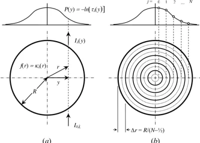
Abel’s integral equation arises in many areas of science and engineering, notably in combustion problems in which the radial distribution of a quantity in an axisymmetric flame is inferred from line-of-sight measurements made through the flame. An example of such an experiment is shown in Fig. 1 (a) where the objective is to determine the spectral absorption coefficient distribution from laser attenuation measurements taken at evenly-spaced axial locations. After some geometric analysis, it can be shown that transmittance measurements P(y) = −ln[τλ(y)] are related to the local spectral absorption
coefficient f(r) = κλ(r) by
(1) which is a form of Abel’s integral equation. In the generic form of Abel’s equation f(r) is called the field variable, while
P(y) is the projected data. Flame temperature measurements
made by emission/absorption pyrometry [1] and Schlieren imaging [2] also involve equations of a similar form.
Abel’s integral equation is a Volterra integral equation of the first-kind, a class of equations that is moderately ill-posed. Unlike most Volterra equations of the first-kind, Abel’s integral equation has a known analytical solution,
(2) where P′(y) = dP(y)/dy. In practice, however, this solution is of limited usefulness because the analytical derivative of the projection data is usually unknown and approximating P′(y) by a finite-difference scheme amplifies experimental error present in the P(y) measurements; this effect is exacerbated as the number of measurement locations increases, limiting the resolution of f(r). On the other hand, using too few P(y) values to estimate P′(y) leads to large errors in f(r) due to truncation of higher-order Taylor series terms.
( )
∫
( )
− ′ − = R y dy r y y P r f 1 , 2 2 πBecause of the ubiquity of Abel’s equation in science and engineering, a large and diverse set of numerical deconvolution methods have been developed for solving Eq. (1). The majority of these techniques belong to one of two classes: those that work directly on Eq. (1), and those that work on Eq. (2). Comprehensive reviews of these methods are provided by Dasch [3] and Gorenflo and Vessella [4].
The simplest and most common of the first type is the onion-peeling method [3], in which the flame field is divided into N evenly-spaced annular elements of thickness ∆r =
R/(N−1/2), as shown in Fig. 1 (b). Assuming f(r) to be uniform
over each element transforms Eq. (1) into
(3) where yi = i∆r, rj = j∆r, Pi = P(yi), and fj approximates f(rj).
Writing Eq. (3) for each annular element gives rise to a set of linear equations that can be rewritten as AOP x = b, where x contains the unknown field variables, xT = {fi,, i = 0, 1, ..., Ν−1} and b contains the projected data set, bT
= , 2 1 1 2 , 2 , 2 2
∑
−∫
= ∆ + > ∆ − = − = N j r r i j r r i j r i j i j j i dr y r r f P( )
2( )
, 2 2∫
− = R y dr y r r r f y P{P(ri),, i = 0, 1, ..., Ν−1}; because AOP is an upper-triangular matrix, x is readily solved for by back-substitution.
Another way of solving Eq. (1) is by filtered back-projection, a technique originally developed for multi-dimensional medical imaging applications [5] and later adapted to perform one-dimensional deconvolution [3]. In this approach, a Fourier analysis is used to transform Eq. (1) into its frequency space. Next, the transformed P(y) distributions measured from different view angles is “back-projected” over the field domain to recover f(r) in the frequency space. (In this application, the number of view angles is infinite due to axial symmetry.) Although the back-projection step filters out experimental error, active filtering techniques are also sometimes employed to smooth P(y) in the frequency space.
The techniques belonging to the second class of deconvolution can be divided into two subclasses. Those of the first subclass work by finding an easily-differentiable function
( )
yP~ that approximates a subset of the projected data [6, 7, 3], and then substituting it into Eq. (2) to find an estimate of f(r). Of these techniques, Abel three-point inversion [3] has become one of the most popular deconvolution techniques used in combustion applications. In this approach, P~i
(
y,Pi−1,Pi,Pi+1)
is a quadratic that approximates P(y) over the interval yi – ∆r/2
= y = yi + ∆y/2 by interpolating the subset {Pi−1, Pi, and Pi+1}. The domain of integration in Eq. (2) is divided into N evenly-spaced subdomains, and the corresponding P~i
(
y,Pi−1,Pi,Pi+1)
is then substituted into each integral to give
(4) (At r = 0, Pj−1 is set equal Pj+1 so that P′(0) = 0, and Pj+1 = 0 at r = R.) Carrying out the integration over each subinterval results in N linear equations that explicitly define fi in terms of the
projected data; these in turn can be rearranged into a matrix equation, x = DAbelb, where x and b are defined as above.
Methods belonging to the second subclass transform Eq. (2) through integration-by-parts into a form that doesn’t involve P′(y), thereby avoiding differentiation of discrete and error-contaminated projected altogether. Examples of this approach are presented in [8-10].
The main drawback of these techniques is their instability, caused by the inherent ill-posedness of Abel’s equation. Small errors in the projected data, inevitable in an experimental setting, are magnified by the deconvolution process into large errors in the field variable distribution. The present work describes how Tikhonov regularization can be applied to stabilize the deconvolution process. Regularization methods work by solving a sequence of well-posed problems formed by modifying, or regularizing, the original ill-posed problem. Well-posed problems that closely resemble the original posed problem have solutions that accurately solve the ill-posed problem, but tend to be large in magnitude and highly oscillatory. As the degree of regularization increases, the
solutions become smoother at the expense of accuracy. Most regularization methods are heuristic in the sense that the analyst must adjust the degree of regularization by varying a
regularization parameter in order to find the optimal trade-off between smoothness and accuracy.
In this paper we first describe the ill-posed nature Abel’s integral equation and demonstrate how this condition is diagnosed, and then show how Tikhonov regularization is applied to solve Abel’s integral equation. Finally, the performance of Tikhonov regularization is compared to that of the onion-peeling and Abel three-point deconvolution methods by solving a contrived problem based on an experimentally determined soot-volume fraction distribution of an axisymmetric flame. The results demonstrate that Tikhonov regularization is less sensitive to experimental error and provides more accurate solutions compared to the other deconvolution methods.
Fig 1: (a) Evaluating spectral absorption coefficient distribution within an axisymmetric flame, and (b) discretrization of the problem domain
NOMENCLATURE A Coefficient matrix
AOP Coefficient matrix of onion-peeling deconvolution
b Right-hand side vector containing projected data δb Vector of perturbations in b
δx Perturbation in solution corresponding to δb
DAbel Coefficient matrix of Abel three-point deconvolution
f(r) Field variable
fi Approximation of f(ri)
Li i
th
derivative operator in discrete space
N Number of discrete field variables/projection locations
P(y) Projected data Pi P(yi) r Radial location
(
)
. , , , ' ~ 1 1 2 2 2 2 1 1 dy r y P P P y P f N i j r y r y i j j j i j j∑ ∫
− = ∆ + ∆ − + − − − = π (a) j = 0 1 2 … N P(y) = −ln[τλ(y)] ∆r = R/(N−½) f(r) = κλ(r) r y R Iλ(y) I0λ (b)R Outer radius of field variable domain
wi i th
singular value
x Vector of unknown field variable values
y Axial location αi i
th
regularization parameter ε Error in projected data
εRMS Root-mean-squared error of {fi}, Eq. (16)
λi i th
eigenvalue
µ Mean value of Gaussian error distribution µi i
th
eigenvector
σ Standard deviation of Gaussian error distribution Subscripts and Superscripts
Abel Abel three-point deconvolution OP Onion-peeling
* Solution/global minimum ~ Approximate value
STABILITY OF DECONVOLUTION METHODS
The formal definition of an ill-posed problem arises from Hadamard’s description of a well-posed mathematical problem [11]. In order for a mathematical problem to be well posed, Hadamard stated that it (1) must have a solution, (2) that the solution must be unique, and (3) the solution must be a continuous function of the inputs. Any problem that doesn’t satisfy all three of the above criteria is ill-posed.
Abel’s integral equation is only mildly ill-posed because the existence and uniqueness of a solution can be demonstrated mathematically, providing that f(r) and P(y) are continuously differentiable [4]. Intuitively, Hadamard’s first criterion is obviously satisfied in an experimental setting, since the projected data is derived from the unknown field distribution. The second criterion is also satisfied since the domain of the integral in Eq. (1) approaches zero as y approaches R, so f(R) is known with certainty. Values of f(r) with r < R are then found from f(r′) where r < r′ = R, in an analogy to onion-peeling in continuous space.
Instead, Abel’s integral equation is ill-posed because it violates Hadamard’s third criterion, i.e. that the solution for f(r) is very sensitive to small perturbations in P(y). This well-known and troublesome property arises when solving Abel’s equation both in its forward form, Eq. (1), and in its inverted form, Eq. (2). When solving Eq. (1) through onion-peeling, for example, rows in AAble become less distinct as N becomes large, leading to a coefficient matrix that is nearly rank-deficient. (An example is shown later in the paper.) Furthermore, errors in the estimation of f(r) accumulate as r approaches 0, since fi is contaminated by errors contained in fj, j
> i as well as the experimental error in Pi. As previously
mentioned, solving Eq. (2) necessitates the approximation of
P′(y) using discrete values of {Pi, i = 0, 1, …, N−1} through
numerical techniques like finite differences, which also tend to magnify errors in the projected data. Rather than considering these error amplification mechanisms independently, both should be thought of as manifestations of the fundamental ill-posed nature of Abel’s integral equation.
The degree of ill-posedness inherent to the solution procedure can be quantified by applying perturbation theory [12] to estimate the sensitivity of a solution to perturbations in the input data. In particular, consider the linear system Ax = b, where vectors x and b contain the field variable and projected data evaluated at discrete values over the domains of r and y, as described above. Suppose the projected data contained in b is contaminated by error contained in δb. The corresponding error in the field variable, δx, is found by
(5)
(
x+δx)
=b+δb, Awhich can be simplified by substituting b = Ax, so that Aδx = δb, or δx = A−1δb. To estimate the magnitude of δx, note from the theory of vector and matrix norms that ||A−1|| ||δb|| ≥ ||A−1δb||, so (6) . 1 b x δ δ ≤ A−
Finally, it is customary to normalize the left-hand side of Eq. (6) so that the stability measurement is independent of the solution magnitude. Noting that ||A|| ||x|| ≥ ||b||, we get
( )
, 1 -b b δ b b δ x x δ A A A ⋅ =Cond ≤ (7)where the condition number of matrix A, Cond(A), indicates the stability of x relative to perturbations in b, or more precisely, the maximum effect a perturbation in b can have on x. In well-posed linear problems, Cond(A) is of order unity, so small perturbations in b do not cause large changes in x; in this case A is said to be well-conditioned. If Cond(A) is large, on the other hand, small changes in b are magnified into large errors in x, in which case A is said to be ill-conditioned. The latter scenario occurs when solving Abel’s integral equation.
The ill-posed nature of Abel’s integral equation is demonstrated by examining the condition numbers of the coefficient matrices that arise when solving Eq. (1) through onion-peeling and Eq. (2) through Abel three-point deconvolution. Since the linear equations defined by the latter method expresses the vector of field variables x explicitly in terms of the projected data contained in b, x = DAbel b, we instead examine the condition number of AAbel = DAbel−1. The condition number of a matrix can be evaluated numerically as the ratio of the largest and smallest singular values of A,
( )
wmax wmin,Cond A = (8)
which in turn are found by performing a singular value decomposition on A, (9) , T V V U A= ⋅ ⋅
where U and VT are two orthogonal matrixes and W is a diagonal matrix containing the singular values.
The condition numbers for AOP and AAbel are plotted in Fig. 2 as a function of the number of discrete field variables/projection locations, N. The condition numbers of both AOP and AAbel both increase linearly with N and are large even at moderate values of N. This behavior limits the field variable resolution that can be achieved in experiments like the one shown in Fig. 1 (a), where measurement errors in the projected dataset are unavoidable. The relative magnitudes of the condition numbers obtained from the onion-peeling and Abel-three point deconvolution techniques suggest that the error magnification by onion-peeling is about 2.25 times worse than the error amplification by Abel three-point deconvolution, i.e. ||δx||OP = 2.25 ||δx||Abel for a given value of N. Although the predicted value of ||δx|| using the condition number can be as much as an order of magnitude greater than the actual value of ||δx||, the relationship between the magnitudes of the condition numbers and relative error amplification of the deconvolution techniques is confirmed later in the paper.
Fig 2: Matrix condition numbers from onion-peeling and Abel three-point deconvolution.
TIKHONOV REGULARIZATION
Problems caused by the ill-posedness of Abel’s integral equation in the deconvolution of projected data can be overcome by using a regularization technique. These techniques work by generating solutions to a sequence of well-posed problems that approximate the exact solution to the original ill-posed problem. Well-posed problems that are closely related to the original ill-posed problem have solutions that solve the ill-posed problem with a very small residual, but these solutions tend to be large in magnitude and highly-oscillatory. On the other hand, well-posed problems that are more distantly related to the original ill-posed problem have smoother but less accurate solutions. The set of well-posed problems is formed by varying a heuristic regularization
parameter; by systematically adjusting this parameter, the
analyst can find a solution that represents an acceptable compromise between accuracy and regularity.
Tikhonov regularization [13] is well-suited for solving ill-conditioned linear systems like the ones described in the previous section. The approach is based on the observation that the quadratic objective function
( )
x xT T x xT TbF = A A − A
2 1
1 (10)
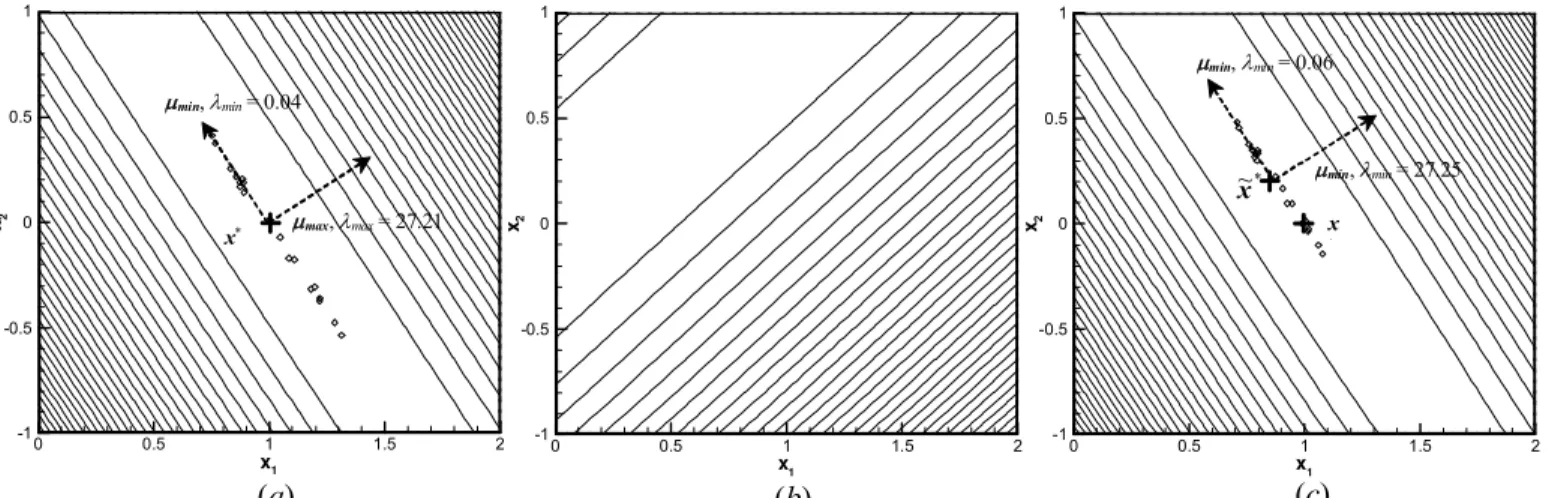
is minimized when x solves the linear set of equations Ax∗ = b, since ∇F1(x) = ATAx−ATb = 0 when x = x∗. If A is ill-conditioned, however, F1(x) will be nearly degenerate, meaning that a strong global minimum is difficult to discern over the domain of x. This condition is shown graphically in Fig. 3 (a) for , 2 4 1 2 5 . 2 4 2 1 b x ⎥= ⎦ ⎤ ⎢ ⎣ ⎡ − − = ⎥ ⎦ ⎤ ⎢ ⎣ ⎡ ⎥ ⎦ ⎤ ⎢ ⎣ ⎡ = x x A (11)
where matrix A is ill-conditioned because it is nearly rank-deficient, since its rows are nearly linearly-dependent. The relationship between the ill-conditioned nature of A (and that of ATA) and the objection function topography shown in Fig. 3 (a) is better understood by noting that at x∗, the ith eigenvalue of ATA, λi, indicates the rate that F1(x) increases as x moves away from x∗ in the direction of the corresponding eigenvector, µi. Furthermore, the condition number of a matrix can
alternatively be defined as the ratio of its largest and smallest eigenvalues, Cond(AT
A) = λmax/λmin. If Cond(ATA) is large
then ATA has at least one very small eigenvalue, λmin, and then
||∇F1(x)|| is small near the line x∗+cµmin. Furthermore, since
∇F1(x) = ATAx−ATb, there is an infinite set of solutions {xi=x∗+δxi} close to line x∗+cµmin that satisfy A(x∗+δxi) =
b+δbi, where δbi represents a small perturbation to the input
data.
140
Onion-Peeling Abel Three-Point
In order to stabilize the solution of Ax = b, a regularizing objective function F2(x) is added to F1(x) to define a new composite objective function, F(x) = F1(x) + F2(x). The regularizing objective function F2(x) is given by
(12) where Li is an approximation of the ith-derivative operator in
discrete space and αi is the regularization parameter. In this
paper, we focus on the 0th-order regularization,
(13)
and αi = 0, i > 0. Accordingly, F2(x) is minimized by a constant solution, xi∗ = C, i = 1, 2, …, N. Because L0 has one more column than row, F2(x) is also degenerate as shown in
( )
∑
= = n i i T i T i F 0 2 x α x L L x, , 1 1 0 0 0 1 1 0 0 0 1 1 0 ⎥ ⎥ ⎥ ⎥ ⎥ ⎥ ⎦ ⎤ ⎢ ⎢ ⎢ ⎢ ⎢ ⎢ ⎣ ⎡ − − − = L O O O M M O L L 0 20 40 60 80 100 1 02 Cond(AOP) = 2.554 N Cond(AAbel) = 1.134 N Cond(A) 0 10 200 300 400 500 NFig. 3 (b). Nevertheless the sum of F1(x) and F2(x) is non-degenerate, having a well-defined global minimum as shown in Fig. 3 (c) that can be found by setting ∇F
* x
~
1(x~* )+∇F2(~x*) = 0 and solving the resulting matrix equation,
(14) The solution to Eq. (14) is a trade-off between a highly-accurate solution that minimises F1(x) and a smooth solution that minimizes F2(x). In a topographical sense, increasing α0 improves stability by “steepening” the curvature of F(x) in the vicinity of , thereby reducing the magnitude of the perturbations δx
* ~
x
i that solve A(~x*+δxi) = b+δbi for a given
magnitude of δbi. This is done at the expense of solution
accuracy, however, since ~x* moves further away from x∗ as α0 is increased and F2(x) becomes larger.
In the present application, Tikhonov regularization is used to regularize the matrix equation arising from onion-peeling deconvolution, so AOP is substituted in place of A in Eq. (14). The analyst must heuristically select a suitable value of α0 that gives a sufficiently smooth and accurate solution for a particular ill-posed problem; a methodology for doing this is presented in the next section.
Finally, it should be noted that onion-peeling and Abel-three point inversion are themselves regularization methods, since their solutions only approximately solve Eqs. (1) and (2), respectively. Onion-peeling regularizes by forcing f(r) to be uniform over the domain ri−∆r/2 ≤ r ≤ ri+∆r/2 while Abel
three-point inversion regularizes by approximating P(y) with a
smooth function over yi−∆r/2 ≤ y ≤ yi+∆r/2. In both cases, the
regularization parameter is the number of discrete annular locations, N; increasing N improves the solution accuracy at the expense of solution stability.
DEMONSTRATION OF METHOD
(
ATA+α0LTL)
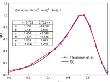
~x*=ATb, In order to demonstrate the use of Tikhonov regularizationas a deconvolution method, it is applied to invert simulated experimental data based on laser attenuation measurements of the soot-volume fraction distribution within an axisymmetric flame estimated [14]. The field variable distribution is a piecewise function f(r) composed of two 4th
-order polynomials that has a shape resembling the normalized experimental data; the curve has the properties f′(0) = 0, f(1) = 0, Max[f(r)] = 1, and is at least C1 continuous over its domain. A plot of f(r) and the normalized experimental data is shown in Fig. 4.
Next, the set of projected data is generated by numerically integrating Eq. (1) at discrete values of y. In order to simulate data taken in an experimental setting, the projected data is contaminated with random errors
(15)
(
,)
, 0,1, , 1, ~ = + = − N i P Pi i ε σ µ Kwhere ε(σ, µ) is a random error characterized by a Gaussian distribution with σ = 0.01 and µ = 0, which is consistent with errors found in experimentally-determined projection data [14]. This level of error is also much larger than the error caused by truncation in the numerical integration algorithm.
Fig. 3: Plots of (a) F1(x), (b) F2(x) with α0 = 0.01, and (c) F(x) = F1(x)+F2(x) corresponding to Eq. (11). Diamonds
show solutions obtained by perturbing b with randomly-generated δb vectors with ||δb|| < 0.2.
x1 x2 0 0.5 1 1.5 2 -1 -0.5 0 0.5 1 x∗ µmin, λmin = 0.04 µmax, λmax = 27.21 (a) x1 x2 0 0.5 1 1.5 2 -1 -0.5 0 0.5 1 (b) (c) x1 x2 0 0.5 1 1.5 -1 -0.5 0 0.5 1 x ∗ * ~ x µmin, λmin = 0.06 µmin, λmin = 27.25 2
Fig 4: Field variable distribution and normalized soot-volume fraction data.
As previously mentioned, the analyst must identify a suitable level of regularization to obtain a field variable distribution that is both smooth and accurate. This can be done with the aid of an L-curve, formed by plotting the solution and residual norms obtained using different levels of regularization. Points on the upper-left part of the curve represent under-regularized solutions that accurately solve the linear equation
AOPx = b but are also highly oscillatory due to the contamination of b with experimental error. Points on the lower-right portion of the curve belong to over-regularized solutions that are smooth but do not accurately model f(r). The
L-curve shown in Fig. 5 for N = 20 indicates that the correct
level of regularization lies within the range 10−3 ≤ α0 ≤ 1, since this level is sufficient to smooth out the largest oscillations in
f(r) caused by experimental error without over-regularizing.
Close examination of the solutions obtained using this range of regularization, shown in Fig. 6, lead us to choose α0 = 0.1 for the remainder of the analysis. (The regularization parameter should be re-evaluated for every different value of N since AOP becomes more ill-conditioned as N increases, but we use α0 = 0.1 for all subsequent values of N to simplify the analysis.)
Figures 7 and 8 show results obtained using onion peeling, Abel three-point, and Tikhonov methods to recover f(r) from sets of 20 and 100 points of perturbed projection data. (All methods used the same perturbed data set for each value of N.) In both cases, the data obtained by Tikhonov regularization most closely matches the exact field variable distribution, followed by sets obtained by Abel three-point and onion peeling deconvolutions. Also, while the magnitude of the oscillations in the Tikhonov solution increase only slightly between N = 20 and N = 100, those in the other solutions grow dramatically with increasing N due to the large condition number of the governing equations, as indicated by Fig. 2. In practice, the small oscillations in the Tikhonov solution could be filtered out by increasing α0 as N increases, although again this is not done here.
Fig. 5: L-curve for N = 20.
Fig. 6: Tikhonov solutions obtained using different levels of regularization at N = 20.
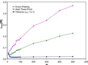
The performance of the three deconvolution techniques is quantified by measuring the accuracy of their solutions using the parameter
(16) Each data point in Fig. 9 represents the average of 100 εRMS(N)
values generated from independently perturbed projected data. Figure 9 shows that solutions obtained using Tikhonov regularization are more accurate than those found using the onion-peeling and Abel-three point methods at all values of N. Furthermore, while the errors in the solutions obtained using onion peeling and Abel three-point increase with increasing N, the error in the Tikhonov data remains approximately constant. This suggests that Tikhonov regularization is particularly well-suited for solving problems where the projected data is measured at small intervals (high spatial resolution). Also note that the errors associated with onion peeling are roughly twice as large as those obtained using Abel three-point inversion at a 1.2
( )
1[
~( )
]
. 2 1 1 2 ⎪⎭ ⎪ ⎬ ⎫ ⎪⎩ ⎪ ⎨ ⎧ − =∑
= N i i i RMS f f r N N ε 0.0 0.2 0.4 0.6 0.8 1.0 0.0 0.2 0.4 0.6 0.8 1 r f( r) r < 0.702 0.702 ≤ r a 0.186 −43.868 b −0.411 3.515 c 1.430 43.546 d −2.631 16.835 e 1.509 1.675 φ −1.096 1.269 f(r)= a(r−φ)4+b(r−φ)3+c(r−φ)2+d(r−φ)+e Thomson et al. f(r) 0.65 0.67 0.69 0.71 0.73 0.75 -16 -14 -12 -10 -8 -6 -4 -2 0 log10(||AOPx−b||) log 10 (||x||) α0 =10−8 α0 = 10−2 α0 =10−1 α0 = 1 0 0.2 0.4 0.6 0.8 1.0 1.2 0 0.1 0.2 0.3 0.4 0.5 0.6 0.7 0.8 0.9 1 r f(r) α0 = 10−3 α0 = 10−2 α0 = 10−1 α0 = 1 Exact Solutiongiven value of N, and that both errors grow linearly with N; these results are consistent with the stability analysis of the two methods performed above.
Fig. 7: Field distributions obtained from perturbed projected data, N = 20.
Fig. 8: Field distributions obtained from perturbed projected data, N = 100.
CONCLUSIONS AND FUTURE WORK
This paper demonstrates how Tikhonov regularization can be applied to solve inverse tomography problems governed by Abel’s integral equation. Tikhonov regularization stabilizes the deconvolution process by adding a regularizing matrix to the ill-conditioned set of equations obtained from onion-peeling deconvolution, transforming it into a well-conditioned set of equations. The performance of this method was assessed by using it to solve the distribution of a known field variable from sets of N projected data points, each contaminated with artificially-generated experimental error. The field variable distribution found using Tikhonov regularization was less sensitive to perturbations in the projected data compared with those obtained from unregularized onion-peeling and Abel three-point inversion techniques at all values of N.
Furthermore, the Tikhonov solution remained stable at large values of N compared to those of the other two methods, which became increasingly sensitive to experimental error as N increases. The latter result is particularly important for problems in which many projected data points are needed to accurately resolve f(r).
This study will shortly be extended to include comparisons of Tikhonov regularization to filtered back-projection and derivative-free deconvolution methods. We also intend to evaluate Tikhonov regularization as a tool to solve nonlinear deconvolution problems that arise in emission/absorption tomography experiments involving optically-thick flames.
Fig. 9: Accuracy of field distributions obtained from perturbed projected data.
ACKNOWLEDGMENTS
The authors wish to thank Dr. DK Ezekoye at the University of Texas at Austin for suggesting this research.
REFERENCES
[1] Hall, R. J. and Bonczyk, P. A., 1990, “Sooting Flame Thermometry using Emission/Absorption Tomography,” Applied Optics, 29, 4590-4598.
[2] Schwarz, A., 1996, “Multi-tomographic Flame Analysis with a Schlieren Apparatus,” Measurement Science and Technology, 7, pp. 406-413.
[3] Dasch, C. J., 1992, “One-Dimensional Tomography: A Comparison of Abel, Onion-Peeling and Filtered Backprojection Methods,” Applied Optics, 31, 1146-1152.
[4] Gorenflo, R. and Vessella, S., 1991, Abel Integral Equations: Analysis and Applications, in Lecture Notes in
Mathematics, A. Dold et al. eds., Springer, Berlin.
[5] Ramachandran, G. N., and Lakshminarayanan, A. V., 1971, “Three-Dimensional Reconstruction from Radiographs and Electron Micrographs: Applications of Convolutions instead of -0.6 -0.4 -0.2 0.0 0.2 0.4 0.6 0.8 1.0 1.2 1.4 0 0.1 0.2 0.3 0.4 0.5 0.6 0.7 0.8 0.9 1 r f(r) Onion-Peeling Abel Three-Point Tikhonov (α0 = 0.1) Exact Solution -0.2 0.0 0.2 0.4 0.6 0.8 1.0 1.2 0 0.1 0.2 0.3 0.4 0.5 0.6 0.7 0.8 0.9 1 r f(r) Onion-Peeling Abel Three-Point Tikhonov (α0 = 0.1) Exact Solution 0.0 0.1 0.2 0.3 0.4 0.5 0 100 200 300 400 500 600 N εrm s (N) Onion-Peeling Abel Three-Point Tikhonov (α0 = 0.1)
Fourier Transforms,” Proceedings of the National Academy of Sciences, 69, pp. 2236-2240.
[6] Cremers, C. J., and Birkebak, R. C., 1966, “Application of the Abel Integral Equation to Spectrographic Data,” Applied Optics, 5, pp. 1057-1063.
[7] Deutsch, M., and Beniaminy, I., 1983, “Inversion of Abel’s Integral Equation for Experimental Data,” Journal of Applied Physics, 54, pp. 137-143.
[8] Anderssen, R. S., 1976, “Stable Procedures for the Inversion of Abel’s Equation,” Journal of the Institute of Mathematics and Its Applications, 17, pp. 329-342.
[9] Chan, C. K., and Lu, P., 1981, “On the Stability of the Solution of Abel’s Integral Equation,” Journal of Physics A: Mathematical and General, 14, pp. 575-578.
[10] Deutsch, M., and Beniaminy, I., 1982, “Derivative-Free Inversion of Abel’s Integral Equation,” Applied Physics Letters, 41, pp. 27-28.
[11] Hadamard, J., 1923, Lectures on Cauchy’s Problem in
Linear Differential Equations, Yale University Press, New
Haven, CT.
[12] Gill, P. E., Murray, W., and Wright, M. H., 1981, Practical
Optimization, Academic Press, San Diego, CA, pp. 28-30.
[13] Tikhonov, A. N., 1975, Inverse Problems in Heat Conduction, Journal of Engineering Physics, 29, (1), pp. 816-820.
[14] Thomson, K. A., Güilder, Ö. L., Weckman, E. J., Fraser, R. A., Smallwood, G. J., and Snelling, D. R., 2005, Soot Concentration and Temperature Measurements in Co-Annular, Nonpremixed CH4/Air Laminar Flames at Pressures up to 4 MPa, Combustion and Flame, 140, pp. 222-232.