Integral approach to sensitive singular perturbations

The immediate aim of this project is to examine across cultures and religions the facets comprising the spirituality, religiousness and personal beliefs domain of quality of life

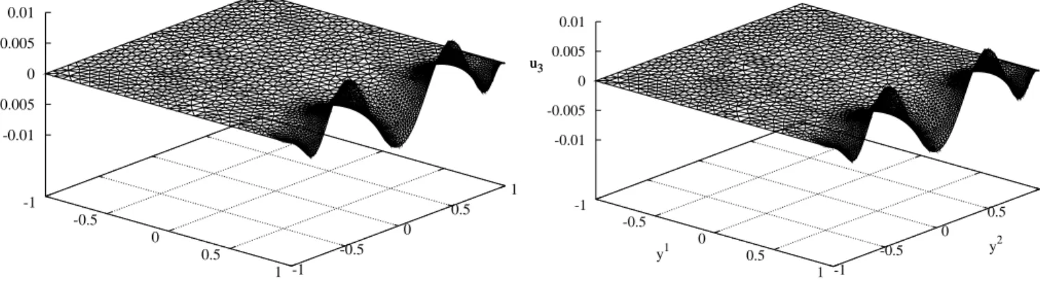
The main purpose of this paper is to give general ideas on a kind of singular perturbations arising in thin shell theory when the middle surface is elliptic and the shell is fixed by

Moreover, in boundary value problems for partial differential equations, the variational theory is obviously associated with finite element approximation.. In certain cases at

In a first section, we give the full asymptotic expansion of the state function in the case of a straight boundary near the origin, this is based on a multiscale asymptotic method..

In order to apply the results of the preceding chapters to singular perturbations of elliptic boundary value problems, it is necessary to know when the solution of degenerate problem

Many different methods have been used to estimate the solution of Hallen’s integral equation such as, finite element methods [4], a general method for solving dual integral equation

We construct 2-surfaces of prescribed mean curvature in 3- manifolds carrying asymptotically flat initial data for an isolated gravitating system with rather general decay

Suppose R is a right noetherian, left P-injective, and left min-CS ring such that every nonzero complement left ideal is not small (or not singular).. Then R