Publisher’s version / Version de l'éditeur:
Vous avez des questions? Nous pouvons vous aider. Pour communiquer directement avec un auteur, consultez
la première page de la revue dans laquelle son article a été publié afin de trouver ses coordonnées. Si vous n’arrivez pas à les repérer, communiquez avec nous à [email protected].
Questions? Contact the NRC Publications Archive team at
[email protected]. If you wish to email the authors directly, please see the first page of the publication for their contact information.
https://publications-cnrc.canada.ca/fra/droits
L’accès à ce site Web et l’utilisation de son contenu sont assujettis aux conditions présentées dans le site LISEZ CES CONDITIONS ATTENTIVEMENT AVANT D’UTILISER CE SITE WEB.
The 18th IEEE International Conference on Tools with Artificial Intelligence
(ICTAI06) [Proceedings], 2006
READ THESE TERMS AND CONDITIONS CAREFULLY BEFORE USING THIS WEBSITE. https://nrc-publications.canada.ca/eng/copyright
NRC Publications Archive Record / Notice des Archives des publications du CNRC :
https://nrc-publications.canada.ca/eng/view/object/?id=b265c491-acd0-4b85-9d44-7aa857525974
https://publications-cnrc.canada.ca/fra/voir/objet/?id=b265c491-acd0-4b85-9d44-7aa857525974
NRC Publications Archive
Archives des publications du CNRC
This publication could be one of several versions: author’s original, accepted manuscript or the publisher’s version. / La version de cette publication peut être l’une des suivantes : la version prépublication de l’auteur, la version acceptée du manuscrit ou la version de l’éditeur.
Access and use of this website and the material on it are subject to the Terms and Conditions set forth at
Decision Trees for Probability Estimation: An Empirical Study
National Research Council Canada Institute for Information Technology Conseil national de recherches Canada Institut de technologie de l'information
Decision Trees for Probability Estimation:
An Empirical Study *
Liang, H., Zhang, H., Yan, Y.
November 2006
* published at The 18th IEEE International Conference on Tools with Artificial Intelligence (ICTAI06). November 13-15, 2006. Washington D.C., USA. NRC 48783.
Copyright 2006 by
National Research Council of Canada
Permission is granted to quote short excerpts and to reproduce figures and tables from this report, provided that the source of such material is fully acknowledged.
Decision Trees for Probability Estimation: An Empirical Study
Han Liang
Harry Zhang
Faculty of Computer Science,
University of New Brunswick
Fredericton, NB, Canada E3B 5A3
{w637g, hzhang}@unb.ca
Yuhong Yan
National Research Council of Canada
Fredericton, NB, Canada E3B 5X9
[email protected]
Abstract
Accurate probability estimation generated by learning models is desirable in some practical applications, such as medical diagnosis. In this paper, we empirically study tra-ditional decision-tree learning models and their variants in terms of probability estimation, measured by Conditional Log Likelihood (CLL). Furthermore, we also compare deci-sion tree learning with other kinds of representative learn-ing: na¨ıve Bayes, Na¨ıve Bayes Tree, Bayesian Network, K-Nearest Neighbors and Support Vector Machine with re-spect to probability estimation. From our experiments, we have several interesting observations. First, among various decision-tree learning models, C4.4 is the best in yielding precise probability estimation measured by CLL, although its performance is not good in terms of other evaluation criteria, such as accuracy and ranking. We provide an ex-planation for this and reveal the nature of CLL. Second, compared with other popular models, C4.4 achieves the best CLL. Finally, CLL does not dominate another well-established relevant measurement AUC (the Area Under the Curve of Receiver Operating Characteristics), which suggests that different decision-tree learning models should be used for different objectives. Our experiments are con-ducted on the basis of 36 UCI sample sets that cover a wide range of domains and data characteristics. We run all the models within a machine learning platform - Weka.
1. Introduction
In the areas of machine learning and data mining, clas-sification accuracy has been established as the major crite-rion to evaluate learning models. However, it completely ignores probability estimation generated by models as long as misclassification does not occur. In many real applica-tions, accurate probability estimation is crucial compared with merely classifying unlabeled samples into a fixed num-ber of categories. For instance, in cost-sensitive learning,
the optimal prediction for an unlabeled sample st is the classcjthat minimizes [3]
h(st) = arg min cj∈C X ci∈C−cj ˆ p(ci|st)C(cj, ci), (1)
whereC(cj, ci) indicates the cost of misclassifying stinto ciin a cost matrix C. One can observe that the metric func-tion directly relies on accurate probabilities.
In practice, however, the true probability of unlabeled samples is often unknown given a sample set with class la-bels. Is there any way to measure the probability estimation yielded by a model when the true probability is unknown? Fortunately, the answer is yes. Recently, Conditional Log
Likelihood(CLL) has been proposed and used for this pur-pose [4, 5, 6]. In Equation 2, a formal CLL definition is given. CLL(Γ|S) = n X t=1 log PΓ(C|st), (2) where Γ is a learning model and S is a sample set with
n samples. [4] described that maximizing Equation 2 amounts to best approximate the conditional probability of
Cgiven each unlabeled samplest, and is equivalent to min-imizing the conditional cross-entropy.
Another recently widely-used alternative is the Area
Un-der the ROC Curve, or simply AUC [16]. Assume that a learning model Γ produces the probabilityp(c|sˆ t) for each unlabeled samplest, and that all the unlabeled samples are ranked based onp(c|sˆ t). For binary classification, AUC can be easily computed as follows [7].
AU C(Γ|S) = S+− n+(n++ 1)/2 n+n−
, (3)
wheren+ andn− are the numbers of positive and nega-tive samples respecnega-tively, andS+ =Pri, whereri is the rank ofithpositive sample in the ranking. It can be ob-served that AUC essentially measures the quality of a rank. More precisely, the more negative samples that are listed
preceding positive samples, the larger AUC value we will get. Note that ranking is based on probability estimation, and it would be accurate if the probabilities are accurate. Thus, AUC can be also used to evaluate the probability es-timation of a learning model. However, it seems that AUC is only an indirect evaluation metric.
The liaison between the above two metrics is demon-strated by two instances. Assume thats+ands−are a pos-itive and a negative sample respectively, and their true class probabilities are p(+|s+) = 0.6 and p(−|s−) = 0.5. A learning model Γ, which yields class probability estimates ˆ
p(+|s+) = 0.5 and ˆp(+|s−) = 0.2, gives a correct order of s+ands−in the ranking that results in a good AUC value. Notice that the probability estimation fors− is far inaccu-rate. However, obtaining a relatively better probability esti-mate could not guarantee a good AUC result. Suppose that another model Θ outputs probability estimates fors+ and s− asp(+|sˆ +) = 0.6 and ˆp(+|s−) = 0.6. As we can see Θ works better than Γ in terms of CLL, but it will generate a worse AUC result sinces+ ands− share the same posi-tive probability and will be ordered randomly, which could greatly aggravate the AUC value.
Decision trees are well known as a typical learning model for classification accuracy, although it has been ob-served that traditional decision trees produce poor probabil-ity estimation [18]. A variety of methods have been pro-posed to learn decision trees for accurate probability esti-mation [17, 14, 12], and AUC is often used as the measure-ment. Huang and Ling [9] empirically studied the perfor-mance of various learning models in terms of AUC. As we notice, it seems that CLL is a more straightforward mea-surement to evaluate learning models with respect to prob-ability estimation. How about the performance of learning models in terms of CLL? What is the relation between CLL and AUC? These are the key motivations of the paper. We primarily focus on decision tree learning. We first system-atically investigate the use of CLL as the performance met-ric to evaluate tree-related models. In particular, as a case study, we compare C4.4 (the improvement version of C4.5 for better probability estimation) and its variants, with C4.5 ( traditional decision tree) and its variants in terms of CLL performance. Second, we also experimentally study sev-eral commonly-used models, such as TAN and SVM, with the purpose of which model is currently best in generating accurate probability estimation. The paper concludes with several observations. (1) Among tree-related models, C4.4 is best in yielding accurate probability estimation. (2) In the domain of classic learning models, C4.4 is also the best in terms of accurate probability estimation. (3) The induc-tive associations between AUC and CLL under decision tree learning paradigms are as well introduced.
This paper is outlined as follows: Section 2 reviews re-cent work on improving decision trees for better probability
estimation. Section 3 introduces the experiment configura-tion and methodology. In Secconfigura-tion 4 empirical results are analyzed and discussed, and we will close our paper in Sec-tion 5 by drawing our inclusions and presenting the further work.
2. Optimizing Probability Estimation
In a decision boundary-based theory, an explicit decision boundary is induced from a set of labeled samples, and an unlabeled samplestis categorized into class cj if stfalls into the decision area corresponding tocj. However, tradi-tional decision trees, such as C4.5 [20] and ID3 [19], have been observed to produce poor probability estimation [18]. Normally, decision trees produce probabilities by comput-ing the class frequencies from the sample sets at leaves. For example, assuming there are 30 samples at a leaf, 20 of which are in the positive class and others belong to the negative class. Therefore, each unlabeled sample that falls into that leaf will be assigned the same probability estimates (pˆ+(+|st) = 0.67 (20/30) and ˆp−(−|st) = 0.33(10/30)). Equation 4 gives a formal expression.
ˆ
p(cj|st) = ncj
n , (4)
here, ncj is the number of samples that belong to class
cj and n is the total number of samples at this leaf. Due to using Information Gain or Gain Ratio as splitting met-rics, traditional tree inductive algorithms prefer a small tree with a substantial amount of samples at leaves and try to make leaves pure. This will incur two major problems. (1) Many unlabeled samples will share the same probability es-timates, which definitely biases against producing accurate probability estimation. In addition, the resulting probabili-ties will be systematically shifted towards zero or one. (2) Decision trees adopt some pruning techniques, such as
ex-pected error pruningor pessimistic error pruning, for high classification accuracy. However, some branches, which make no sense of improving accuracy but contribute to get accurate probability estimation, will be removed.
Because of this, learning decision trees that accurately estimate the probability of class membership, called
Prob-ability Estimation Trees(PETs), has attracted much atten-tion. Provost and Domingos [17] presented a few of such techniques to modify C4.5 for better probability estimation. First, using Laplace correction at leaves, probability esti-mates can be smoothed towards the prior probability distri-bution. Second, by turning off pruning and collapsing in C4.5, decision trees can generate larger trees to give more precise probability estimation. The final version is called C4.4. They also pointed out that bagging, an ensemble method that most of the improvement is due to aggregation of probabilities of a suite of trees, could greatly calibrate probability estimation of decision trees.
Ferri et al. [14] introduced another approach, call m-Branch, to tune probability estimates at leaves. m-Branch is a recursive root-to-leaf extension of the m probability esti-mation, in which, for each leaf, the probability estimates are generated by propagating the probability estimates of each of its parent nodes from the root down to itself. Equation 5 is the formal expression of m-Branch method:
ˆ
pchild(cj|st) =
ncj+ m ∗ ˆP pparent(cj|st) cj∈Cncj + m
, (5)
where parameter m is adjusted by the depth and cardinality of the node, andncj is the number of samples that belong
to classcjwithin the node.
Ling and Yan [12] presented their work to augment de-cision trees with respect to better AUC. They described a novel algorithm, in which, for any given unlabeled sample st, instead of using the labeled samples at the leaf where st falls into, the probability estimates are the averages of probability estimates from all the leaves of this tree. The contribution of each leaf is decided by the number of un-equal parent attribute values (parent attributes are defined as the attributes on the path from the root to a leaf) that the leaf has, compared tost.
Deploying a kernel model at each leaf to produce distinct probability estimates is also an alternative solution to over-come the deficiencies of decision trees. Kohavi [10] pro-posed a hybrid model, called Na¨ıve Bayes Tree (NBTree), which uses decision tree as the general structure and de-ploys na¨ıve Bayes at the leaves. The intuition behind it is that: in comparison with decision trees, na¨ıve Bayes works relatively better when the sample set is small. [10] proved that NBTree greatly improves the classification accuracy, but it didn’t mention the probability estimation performance of NBTree. Based on the labeled samples at a leaf, NBTree denotesp(cˆ j|st) as below:
ˆ
p(cj|A(L)) = αˆp(Al(L)|cj, Ap(L))ˆp(cj|Ap(L)), (6) where α is a normalization factor. A(L) is the com-bined set of leaf attributes Al(L) and path attributes Ap(L). All decomposed terms are conditional probabili-ties of Ap(L). ˆp(cj|Ap(L)) is the conditional probability on path attributes. p(Aˆ l(L)|cj, Ap(L)) is the na¨ıve Bayes deployed at this leaf. From the conditional independence assumption of na¨ıve Bayes, the following equation stands: ˆ
p(Al(L)|cj, Ap(L)) = Q n
i=1p(Aˆ li(L)|cj, Ap(L)) where Ali(L) is an individual leaf attribute and n represents the number of leaf attributes.
Another related work involves Bayesian networks [15]. Bayesian networks are directed acyclic graphs that encode conditional independence among a set of random variables. Each variable is independent of its non-descendants in the graph given the state of its parents. Tree Augmented Na¨ıve
Bayes(TAN), proposed by [4], approximates the interaction between attributes by using a tree structure imposed on the na¨ıve Bayesian framework. Indeed, decision trees divide a sample space into multiple subspaces and local condi-tional probabilities are independent among those subspaces. Therefore, attributes in decision trees can repeatedly ap-pear, while TAN describes the joint probabilities among at-tributes, so each attribute appears only once.
3. Experiments
3.1. Model Introduction and Organization
Most methods for improving decision trees aim at ob-taining their probability estimation measured by AUC. However, can they also produce better results in CLL? And how about other classical models work with reference to CLL? We conducted an empirical study to answer a series of relevant questions.
The details of models compared in our experiments are depicted as follows.
C4.5-L: C4.5 (traditional decision tree [20]) with
Laplace correction at leaves. Here, we use Laplace cor-rection at leaves to avoid the zero-frequency problem.
C4.5-L&B: C4.5 with bagging and Laplace correction at leaves.
C4.4: an improved decision tree model for better proba-bility estimation [17].
C4.4-B: C4.4 with bagging.
C4.5-M: C4.5 with m-Branch [14] applied. C4.4-M: C4.4 with m-Branch applied.
C4.5-LY: C4.5 with the Ling&Yan’s algorithm [12] ap-plied.
C4.4-LY: C4.5 with the Ling&Yan’s algorithm applied. NB: na¨ıve Bayes.
TAN: an extended tree-like na¨ıve Bayes [4]. The im-proved ChowLiu algorithm is used to learn the structure.
NBTree: the hybrid model of decision tree and na¨ıve Bayes [10].
KNN-5: a typical lazy model that finds k nearest labeled samples as the neighbors of an unlabeled samplest. KNN generates probability estimation via simply voting among the class labels in the neighborhood, described in Equa-tion 7. ˆ p(cj|st) = 1 +Pni=1I{ci= cj} ´wi o+Pni=1w´i , (7)
whereci is the class label of a neighbor with index i, the indicator function I{x = y} is one if x = y and zero other-wise,w´iis the weight for the neighbor (the default value is one) and o represents the number of class values. We assign
SVM: with the help of linear kernels, the sequential
min-imal optimizationalgorithm has been used to train a SVM model. We use logistic regression models to improve the yielded probabilities. [8] and [21] have introduced in par-ticular the procedure of generating multi-class probability estimation for SVM.
We conducted two groups of experiments. First, we sys-tematically studied the performances of tree-related models in producing accurate probability estimation. In this group, C4.5, C4.4 and their PET variants (L, M, C4.5-LY, C4.5-L&B, C4.4-M, C4.4-LY and C4.4-B) were com-pared. Then, we empirically learned the efficacy of several popular learning models for probability estimation. C4.4, NBTree, NB, TAN, KNN-5 and SVM had been considered in the second group. Furthermore, we also analyzed the be-haviors of these classical models provided that the sample set is a large or binary-class one.
3.2. Experiment Setup and Methodology
For the purpose of our study, we used 36 well-recognized sample sets recommended by Weka [22]. Table 1 is a brief description of these sample sets. All sample sets came from the UCI repository [1]. The preprocessing stages of sam-ple sets were carried out within the Weka platform, mainly including four steps:
1. Applying the filter of ReplaceMissingValues in Weka to replace the missing values of attributes.
2. Applying the filter of Discretize in Weka to discretize numeric attributes. Therefore, all the attributes are treated as nominal.
3. It is well known that, if the number of values of an attribute is almost equal to the number of samples in a sample set, this attribute does not contribute any in-formation to classification. So we used the filter of
Re-movein Weka to delete these attributes. Three occurred within the 36 sample sets, namely Hospital Number in sample set Horse-colic.ORIG, Instance Name in sam-ple set Splice and Animal in samsam-ple set Zoo.
4. Due to the relatively high time complexity of KNN and SVM, we apply the filter of unsupervised Resample in
Wekato re-select sample set Letter and generate a new sample set named Letter-2000. The selection rate is 10%.
Besides, in our experiments, Laplace correction was ap-plied as one of the following forms. Assuming that there are ncj samples that have the class label ascj,t total samples
andk class values in a sample set. The frequency-based probability estimation calculates the estimated probability by p(cˆ j) =
ncj
t . The Laplace estimation calculates it as
Table 1. Description of sample sets used for the experiments. We downloaded these sam-ple sets in the format of arff from the main web page of Weka.
Data Set Size Attr. Classes Missing Numeric
anneal 898 39 6 Y Y anneal.ORIG 898 39 6 Y Y audiology 226 70 24 Y N autos 205 26 7 Y Y balance 625 5 3 N Y breast ⋄ 286 10 2 Y N breast-w ⋄ 699 10 2 Y N colic ⋄ 368 23 2 Y Y colic.ORIG ⋄ 368 28 2 Y Y credit-a ⋄ 690 16 2 Y Y credit-g ⋆ ⋄ 1000 21 2 N Y diabetes ⋄ 768 9 2 N Y glass 214 10 7 N Y heart-c 303 14 5 Y Y heart-h 294 14 5 Y Y heart-s ⋄ 270 14 2 N Y hepatitis ⋄ 155 20 2 Y Y hypoth. ⋆ 3772 30 4 Y Y ionosphere ⋄ 351 35 2 N Y iris 150 5 3 N Y kr-vs-kp ⋆ ⋄ 3196 37 2 N N labor ⋄ 57 17 2 Y Y letter-2000 ⋆ 2000 17 26 N Y lymph 148 19 4 N Y mushroom ⋆ ⋄ 8124 23 2 Y N p.-tumor 339 18 21 Y N segment ⋆ 2310 20 7 N Y sick ⋆ ⋄ 3772 30 2 Y Y sonar ⋄ 208 61 2 N Y soybean 683 36 19 Y N splice ⋆ 3190 62 3 N N vehicle 846 19 4 N Y vote ⋄ 435 17 2 Y N vowel ⋆ 990 14 11 N Y waveform-5000 ⋆ 5000 41 3 N Y zoo 101 18 7 N Y
⋆ indicates a large sample set; ⋄ indicates a binary-class sample set
ˆ p(cj) =
ncj+1
t+k . In the Laplace estimation,p(aˆ i|cj) is cal-culated by p(aˆ i|cj) =
nicj+1
ncj+vi, wherevi is the number of
values of attributeAiandnicj is the number of samples in
classcjwithAi= ai.
We implemented AUC metric, CLL metric, m-Branch method, Ling&Yan’s algorithm within Weka, and used the current versions of learning models and bagging method in
Weka. We learned that using the percentage of the subset as the confusion factor in Ling&Yan’s algorithm was bet-ter than the proposed optimal paramebet-ter 0.3. Therefore, we used a new confusion factor in our experiments. Multi-class AUC has been calculated by M-measure [7]. In all ex-periments, the AUC and CLL results for each model were measured via a 10-fold cross validation 10 times. Runs with various models were carried out on the same train sets and evaluated on the same test sets. In particular, the cross-validation folds were the same for all the experiments on each sample set. Finally, we conducted two-tailed t-test [13] with a significantly different probability of 0.95,
which means that we speak of two results as being “signifi-cantly different” only if the difference is statistically signif-icant at the 0.05 level according to the corrected two-tailed t-test. Also, each entry w/t/l in all t-test tables indicates that the model in the corresponding row winsw sample sets, ties int sample sets, and loses l sample sets, in contrast with the model in the corresponding column.
4. Result Analysis and Discussion
In Table 2 and its t-test summary Table 3, C4.4 is the optimal option among decision tree families when ac-curate probability estimation is desired. Compared with traditional decision trees, C4.4 wins C4.5-L in 10 sample sets, ties in 21 sample sets and loses 5 sample sets. Note that C4.4 adopts both Laplace correction at leaves and turn-ing off prunturn-ing, therefore, we learned that stoppturn-ing prunturn-ing could significantly improve the quality of probability esti-mation. Compared with bagged decision trees, C4.4 wins C4.5-L&B in 16 sample sets and loses 9 samples sets; C4.4 wins C4.4-B in 20 sample sets and loses 8 sample sets.
Bagging is a voting strategy among a group of candidate trees. [17] has proved that bagging is useful in improv-ing probability-based rankimprov-ing. However, accordimprov-ing to our observation of the empirical results of C4.4 and C4.4-B,
baggingis not profitable in producing precise probability estimation. In addition, the comparison results of C4.5-L and L&B are also persuadable: L wins C4.5-L&B in 16 sample sets and loses 8 sample sets. Compared to decision trees with m-Branch, C4.4 outperforms C4.5-M and C4.4-M in 15 sample sets and 13 sample sets respec-tively, and loses 6 sample sets for both of them. For apply-ing Lapply-ing&Yan’s algorithm on decision trees, C4.4 is signif-icantly better than C4.5-LY and C4.4-LY in 33 sample sets and loses no sample set. Thus, we can learn that neither m-Branch method nor Ling&Yan’s algorithm could calibrate decision trees for accurate probabilities.
Most methods mentioned in Section 2 are intended to im-prove probability-based ranking measured by AUC. AUC is a relative evaluation standard. In other words, the cor-rectness of ranking, which depends on the relative position of a sample among a set of others, determines the final re-sult. CLL is directly calculated via adding up log values of probability estimates generated by a learning model for unlabeled samples (see Equation 2). Therefore, in the dia-gram of decision tree learning, CLL and AUC represent two aspects of probability estimation: reliability and res-olution. Dawid [2] described these two conceptual criteria for studying how effective probability predictions are.
Re-liabilitydescribes the probability estimation should be reli-able and accurate, that is, when we assign a positive class probabilityp(+|e) to an event e, there should be roughlyˆ 1 − ˆp(+|e) of the negative class probability for the event
not occurring. Resolution presents that events should be easily ranked in terms of their probabilities. As a result, for decision tree learning, CLL can be employed as evalu-ating the reliability of probability estimation, and AUC will be applied for scaling its resolution performance. In our ex-periments, we also obtained the AUC values of all decision tree models. Table 6 shows thet-test results. We have two valuable observations as follows.
1. Although C4.4 performs best in terms of CLL, all the variants of C4.4 and C4.5 proposed for improving AUC outperforms C4.4 in terms of AUC (see Table 6), which repeated the research results reported by other researchers.
2. Among all the models, C4.4-B achieves the best per-formance on AUC. This means bagging is an effective technique in terms of improving AUC. However, as we noticed before, bagging is not effective in improving CLL.
Now we re-exam CLL in Equation 2. So far, we use the real-world sample sets for our empirical study, i.e. we do not know the real sample distributions. Equation 2 shows that if one model gives higher estimation of p(cˆ j|st) than another, its CLL will be higher. Therefore, CLL favors a model that gives higher probability estimation no mat-ter what the true probability is, since the true probability does not even appear in CLL. Indeed, when using CLL, we imply the assumption that samplest in classcj has prob-ability p(cj|st) = 1 and p(¬cj|st) = 0, thus, there is no surprise that CLL favors a model giving higher probabil-ity estimation. This can explain why C4.4 has better CLL performance than C4.4-B because C4.4 tends to have pure nodes, which means high probability estimation. but bag-ging or other smoothing techniques that tend to smooth the probabilities to avoid high variance. Therefore, CLL is just an indirect evaluation to true probabilities. We can also con-clude that neither CLL nor AUC dominates each other.
In Table 4 and Table 5, we compare C4.4 with non-tree models in terms of CLL. C4.4 achieves significant improve-ment over NB in 17 sample sets and loses 5 sample sets. As an extension of NB in presenting more joint probability dis-tribution, TAN still works poorly compared with C4.4 in 10 sample sets and loses 7 sample sets. Furthermore, t-test results in Table 5 indicates that extending the structure of NB to explicitly represent attribute dependencies (in order to relax the conditional independence assumption of NB) is a good way to improve the performance of probability estimation for NB. TAN achieves substantial progress over NB in 16 sample sets and loses only 3 sample sets. For lazy learning models, C4.4 is better than KNN with k=5 in 12 sample sets. We also conducted a group of compar-isons between C4.4 and KNN with k=10, 30 and 50. Ex-periment results suggested that the bigger k is, the worse
KNN performs in terms of CLL. Due to lack of space, we didn’t show the results of other KNN models with differ-ent values of k. NBTree is proven to be efficidiffer-ent in clas-sification accuracy, but from the results of t-test, it doesn’t work very well compared with other typical models, and is just competitively with NB. Some work [11] has been done to ameliorate NBTree for precise probability estima-tion, where CLL is used as the splitting metric to direct the tree growth process. Although SVM doesn’t work better than C4.4 (wins 7 sample sets and loses 12 sample sets), it is still better than other models, such as NBTree and KNN-5, and competitive with TAN (wins 7 sample sets and loses 8 sample sets). Besides, in AUC comparisons (Table 7), SVM and TAN achieve better results than others.
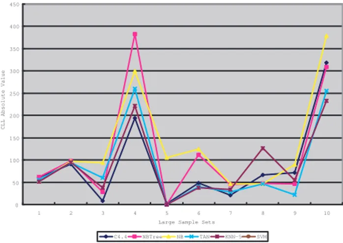
Empirical results on large sample sets in form of CLL absolute values have been demonstrated in Figure 1. We are especially interested in seeing the actual CLL values on large sample sets, because these data sets demonstrate prac-tical cases we can meet. We choose ten sample sets from UCI repository on the condition that the number of sam-ples in each set is above 900. In Figure 1, From No1 to
No10respectively denote the sample sets as German-credit,
Hypothyroid, Kr-vs-kp, Letter-2000, Mushroom, Segment, Sick, Splice, Vowel, Waveform-5000. The plot explored the
0 50 100 150 200 250 300 350 400 450 1 2 3 4 5 6 7 8 9 10
Large Sample Sets
CLL Absolute Value
C4.4 NBTree NB TAN KNN-5 SVM
Figure 1. CLL performance curve on large sample sets
behaviors of classic models when a substantial amount of data is supplied. As we can observe that C4.4 works consis-tently better than others (the lowest learning curve), which stands that C4.4 is the optimal candidate for real-world do-main problems. One valuable observation is that TAN and SVM also work well based on these sample sets. Therefore, TAN and SVM are good options for the cases where classi-fication accuracy plays an important role as well in practice.
Experiments on binary-class sample sets have been also conducted by use of sixteen UCI sample sets:
Breast-cancer, Wisconsin-breast, Horse-colic, Colic.ORIG, Credit-rating, German-credit, Diabetes, Heart-statlog, Hepatitis, Ionosphere, Kr-vs-kp, Labor, Mushroom, Sick, Sonar, Vote
(listed from No1 to No16 in Figure 2). Binary-class sample sets are interesting for us because AUC can be easily calcu-lated for these cases and we can verify results by observing the probability assignments. Figure 2 investigated the
per-0 20 40 60 80 100 120 140 160 180 200 1 2 3 4 5 6 7 8 9 10 11 12 13 14 15 16 Binary-Class Sample Sets
CLL Absolute Value
C4.4 NBTree NB TAN KNN-5 SVM
Figure 2. CLL performance curve on binary-class sample sets
formances of the same models measured by CLL absolute values, and showed that C4.4 is the best option for binary classification problems. In addition, as the plot shows, NB works poorly in some sample sets, such as No11 and No13, where the conditional independence assumption is heavily violated. NBTree and TAN have both relaxed this assump-tion in two different ways (encoding condiassump-tional indepen-dence within tree structure or augmenting the representa-tion ability of joint distriburepresenta-tion), and the curves support that NBTree and TAN work better compared with NB.
5. Conclusions and Future Work
Precise probability estimation provided by learning mod-els is crucial in many real-world applications. In this pa-per, we conduct a systematically experimental study on the probability estimation performances of a group of decision tree variants and other state-of-the-art models, such as SVM and TAN, by use of a newly proposed model quality mea-surement – CLL. Experiments convince us that C4.4 is the best model for CLL among all other models. We point out that CLL is an indirect evaluation of probability estimation and it could work for the real world cases when the true
probability distribution is unknown, however, it favors mod-els which give high probability estimation. We analyze the relationship between AUC and CLL for learning tasks. We include that neither of them dominates the other. For further research, we are going to make similar analyses on artificial data sets with known probability distribution. This will en-able us to theoretically analyze the properties of CLL in de-tail and make a comprehensive contrast between CLL and AUC.
References
[1] C. Blake and C.J. Merz. Uci repository of machine learning database.
[2] A.P. Dawid. Calibration-based empirical probability (with discussion). Annals of Statistics, 13, 1985.
[3] Charles Elkan. The foundations of cost-sensitive learning. In Proceedings of the Seventeenth
Inter-national Joint Conference on Artificial Intelligence, 1991.
[4] N. Friedman, D. Geiger, and M. Goldszmidt. Bayesian network classifiers. Machine Learning, 29, 1997.
[5] D. Grossman and P. Domingos. Learning bayesian network classifiers by maximizing conditional likeli-hood. In Proceedings of the Twenty-First International
Conference on Machine Learning. ACM Press, 2004.
[6] Y. Guo and R. Greiner. Discriminative model selection for belief net structures. In Proceedings of the
Twen-tieth National Conference on Artificial Intelligence. AAAI Press, 2005.
[7] D. J. Hand and R. J. Till. A simple generalisation of the area under the roc curve for multiple class classifi-cation problems. Machine Learning, 45, 2001.
[8] T. Hastie and R. Tibshirani. Classification by pairwise coupling. Annals of Statistics, 26(2), 1998.
[9] J. Huang and C.X. Ling. Using auc and accuracy in evaluating learning algorithms. In IEEE
Trans-actions on Knowledge and Data Engineering, vol-ume 17. IEEE Computer Society, 2005.
[10] Ron Kohavi. Scaling up the accuracy of naive-bayes classifiers: a decision-tree hybrid. In Proceedings of
the Second International Conference on Knowledge Discovery and Data Mining, 1996.
[11] H. Liang and Y. Yan. Learning naive bayes tree for conditional probability estimation. In Proceedings of
the Nineteenth Canadian Conference on Artificial In-telligence. Springer, 2006.
[12] C.X. Ling and R.J. Yan. Decision tree with better ranking. In Proceedings of the Twentieth International
Conference on Machine Learning. Morgan Kaufmann, 2003.
[13] C. Nadeau and Y. Bengio. Inference for the general-ization error. Machine Learning, 52(40), 2003.
[14] C. Ferri P.A. Flach and J. Hernandez-Orallo. Improv-ing the auc of probabilistic estimation trees. In
Pro-ceedings of the Fourteenth European Conference on Machine Learning. Springer, 2003.
[15] J. Pearl. Probabilistic Reasoning in Intelligent
Sys-tems. Morgan Kaufmann, 1988.
[16] F. Provost and T. Fawcett. Analysis and visualiza-tion of classifier performance: Comparison under im-precise class and cost distribution. In Proceedings
of the Third International Conference on Knowledge Discovery and Data Mining. AAAI Press, 1997.
[17] F. J. Provost and P. Domingos. Tree induction for probability-based ranking. Machine Learning, 52(30), 2003.
[18] F. J. Provost, T. Fawcett, and R. Kohavi. The case against accuracy estimation for comparing induction algorithms. In Proceedings of the Fifteenth
Inter-national Conference on Machine Learning. Morgan Kaufmann, 1998.
[19] J. R. Quinlan. Induction of decision trees. Machine
Learning, 2(1), 1986.
[20] J. R. Quinlan. C4.5: Programs for Machine Learning. Morgan Kaufmann: San Mateo, CA, 1993.
[21] C.J. Lin T.F. Wu and R. C. Weng. Probability esti-mates for multi-class classification by pairwise cou-pling. Machine Learning, 5, 2004.
[22] I. H. Witten and E. Frank. Data Mining –Practical
Machine Learning Tools and Techniques with Java Im-plementation. Morgan Kaufmann, 2000.
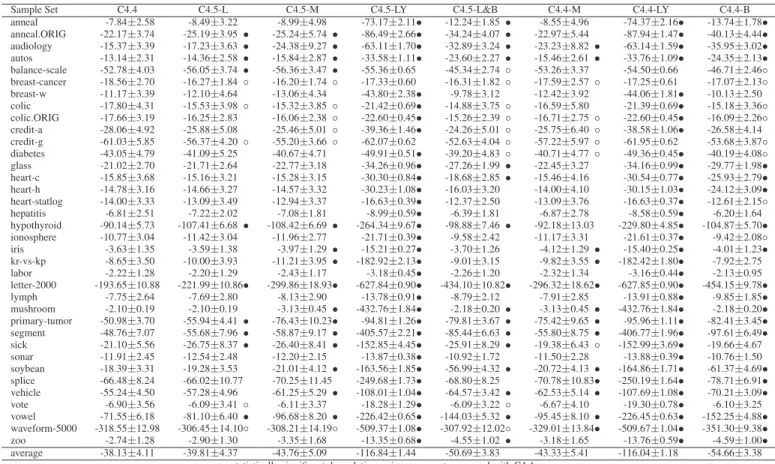
Table 2. Experiment results for C4.4 versus decision tree variants: CLL & standard deviation.
Sample Set C4.4 C4.5-L C4.5-M C4.5-LY C4.5-L&B C4.4-M C4.4-LY C4.4-B
anneal -7.84±2.58 -8.49±3.22 -8.99±4.98 -73.17±2.11• -12.24±1.85 • -8.55±4.96 -74.37±2.16• -13.74±1.78• anneal.ORIG -22.17±3.74 -25.19±3.95 • -25.24±5.74 • -86.49±2.66• -34.24±4.07 • -22.97±5.44 -87.94±1.47• -40.13±4.44• audiology -15.37±3.39 -17.23±3.63 • -24.38±9.27 • -63.11±1.70• -32.89±3.24 • -23.23±8.82 • -63.14±1.59• -35.95±3.02• autos -13.14±2.31 -14.36±2.58 • -15.84±2.87 • -33.58±1.11• -23.60±2.27 • -15.46±2.61 • -33.76±1.09• -24.35±2.13• balance-scale -52.78±4.03 -56.05±3.74 • -56.36±3.47 • -55.36±0.65 -45.34±2.74 ◦ -53.26±3.37 -54.50±0.66 -46.71±2.46◦ breast-cancer -18.56±2.70 -16.27±1.84 ◦ -16.20±1.74 ◦ -17.33±0.60 -16.31±1.82 ◦ -17.59±2.57 ◦ -17.25±0.61 -17.07±2.13◦ breast-w -11.17±3.39 -12.10±4.64 -13.06±4.34 -43.80±2.38• -9.78±3.12 -12.42±3.92 -44.06±1.81• -10.13±2.50 colic -17.80±4.31 -15.53±3.98 ◦ -15.32±3.85 ◦ -21.42±0.69• -14.88±3.75 ◦ -16.59±5.80 -21.39±0.69• -15.18±3.36◦ colic.ORIG -17.66±3.19 -16.25±2.83 -16.06±2.38 ◦ -22.60±0.45• -15.26±2.39 ◦ -16.71±2.75 ◦ -22.60±0.45• -16.09±2.26◦ credit-a -28.06±4.92 -25.88±5.08 -25.46±5.01 ◦ -39.36±1.46• -24.26±5.01 ◦ -25.75±6.40 ◦ -38.58±1.06• -26.58±4.14 credit-g -61.03±5.85 -56.37±4.20 ◦ -55.20±3.66 ◦ -62.07±0.62 -52.63±4.04 ◦ -57.22±5.97 ◦ -61.95±0.62 -53.68±3.87◦ diabetes -43.05±4.79 -41.09±5.25 -40.67±4.71 -49.91±0.51• -39.20±4.83 ◦ -40.71±4.77 ◦ -49.36±0.45• -40.19±4.08◦ glass -21.02±2.70 -21.71±2.64 -22.77±3.18 -34.26±0.96• -27.26±1.99 • -22.45±3.27 -34.16±0.99• -29.77±1.98• heart-c -15.85±3.68 -15.16±3.21 -15.28±3.15 -30.30±0.84• -18.68±2.85 • -15.46±4.16 -30.54±0.77• -25.93±2.79• heart-h -14.78±3.16 -14.66±3.27 -14.57±3.32 -30.23±1.08• -16.03±3.20 -14.00±4.10 -30.15±1.03• -24.12±3.09• heart-statlog -14.00±3.33 -13.09±3.49 -12.94±3.37 -16.63±0.39• -12.37±2.50 -13.09±3.76 -16.63±0.37• -12.61±2.15◦ hepatitis -6.81±2.51 -7.22±2.02 -7.08±1.81 -8.99±0.59• -6.39±1.81 -6.87±2.78 -8.58±0.59• -6.20±1.64 hypothyroid -90.14±5.73 -107.41±6.68 • -108.42±6.69 • -264.34±9.67• -98.88±7.46 • -92.18±13.03 -229.80±4.85• -104.87±5.70• ionosphere -10.77±3.04 -11.42±3.04 -11.96±2.77 -21.71±0.39• -9.58±2.42 -11.17±3.31 -21.61±0.37• -9.42±2.08◦ iris -3.63±1.35 -3.59±1.38 -3.97±1.29 • -15.21±0.27• -3.70±1.26 -4.12±1.29 • -15.40±0.25• -4.01±1.23• kr-vs-kp -8.65±3.50 -10.00±3.93 -11.21±3.95 • -182.92±2.13• -9.01±3.15 -9.82±3.55 • -182.42±1.80• -7.92±2.75 labor -2.22±1.28 -2.20±1.29 -2.43±1.17 -3.18±0.45• -2.26±1.20 -2.32±1.34 -3.16±0.44• -2.13±0.95 letter-2000 -193.65±10.88 -221.99±10.86• -299.86±18.93• -627.84±0.90• -434.10±10.82• -296.32±18.62• -627.85±0.90• -454.15±9.78• lymph -7.75±2.64 -7.69±2.80 -8.13±2.90 -13.78±0.91• -8.79±2.12 -7.91±2.85 -13.91±0.88• -9.85±1.85• mushroom -2.10±0.19 -2.10±0.19 -3.13±0.45 • -432.76±1.84• -2.18±0.20 • -3.13±0.45 • -432.76±1.84• -2.18±0.20• primary-tumor -50.98±3.70 -55.94±4.41 • -76.43±10.23• -94.81±1.26• -79.81±3.67 • -75.42±9.65 • -95.96±1.11• -82.41±3.45• segment -48.76±7.07 -55.68±7.96 • -58.87±9.17 • -405.57±2.21• -85.44±6.63 • -55.80±8.75 • -406.77±1.96• -97.61±6.49• sick -21.10±5.56 -26.75±8.37 • -26.40±8.41 • -152.85±4.45• -25.91±8.29 • -19.38±6.43 ◦ -152.99±3.69• -19.66±4.67 sonar -11.91±2.45 -12.54±2.48 -12.20±2.15 -13.87±0.38• -10.92±1.72 -11.50±2.28 -13.88±0.39• -10.76±1.50 soybean -18.39±3.31 -19.28±3.53 -21.01±4.12 • -163.56±1.85• -56.99±4.32 • -20.72±4.13 • -164.86±1.71• -61.37±4.69• splice -66.48±8.24 -66.02±10.77 -70.25±11.45 -249.68±1.73• -68.80±8.25 -70.78±10.83• -250.19±1.64• -78.71±6.91• vehicle -55.24±4.50 -57.28±4.96 -61.25±5.29 • -108.01±1.04• -64.57±3.42 • -62.53±5.14 • -107.69±1.08• -70.21±3.09• vote -6.90±3.56 -6.09±3.41 ◦ -6.11±3.37 -18.28±1.29• -6.09±3.22 ◦ -6.67±4.10 -19.30±0.78• -6.10±3.25 vowel -71.55±6.18 -81.10±6.40 • -96.68±8.20 • -226.42±0.65• -144.03±5.32 • -95.45±8.10 • -226.45±0.63• -152.25±4.88• waveform-5000 -318.55±12.98 -306.45±14.10◦ -308.21±14.19◦ -509.37±1.08• -307.92±12.02◦ -329.01±13.84• -509.67±1.04• -351.30±9.38• zoo -2.74±1.28 -2.90±1.30 -3.35±1.68 -13.35±0.68• -4.55±1.02 • -3.18±1.65 -13.76±0.59• -4.59±1.00• average -38.13±4.11 -39.81±4.37 -43.76±5.09 -116.84±1.44 -50.69±3.83 -43.33±5.41 -116.04±1.18 -54.66±3.38
•, ◦ statistically significant degradation or improvement compared with C4.4
Table 3. Summary ont-test of CLL experiment results on decision tree variants.
Models C4.5-L C4.5-M C4.5-LY C4.5-L&B C4.4-M C4.4-LY C4.4-B
C4.5-M 2/18/16 C4.5-LY 0/2/34 0/1/35 C4.5-L&B 8/12/16 9/14/13 36/0/0 C4.4-M 4/21/11 7/27/2 34/2/0 13/14/9 C4.4-LY 0/2/34 0/1/35 9/18/9 0/1/35 0/3/33 C4.4-B 6/11/19 7/13/16 35/1/0 2/13/21 6/12/18 35/1/0 C4.4 10/21/5 15/15/6 33/3/0 16/11/9 13/17/6 33/3/0 20/8/8
Table 4. Experiment results for C4.4 versus several classical models: CLL & standard deviation.
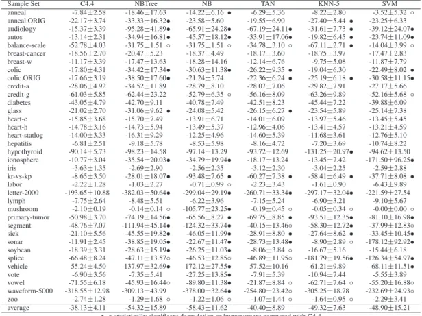
Sample Set C4.4 NBTree NB TAN KNN-5 SVM
anneal -7.84±2.58 -18.46±17.63 -14.22±6.16 • -6.29±5.36 -8.22±2.80 -3.52±5.32 ◦ anneal.ORIG -22.17±3.74 -33.33±16.32• -23.58±5.60 -19.55±6.90 -27.40±5.44 • -23.25±6.33 audiology -15.37±3.39 -95.28±41.89• -65.91±24.28• -67.19±24.11• -31.61±7.73 • -39.12±24.07• autos -13.14±2.31 -34.94±16.81• -45.57±18.12• -33.91±17.06• -19.82±6.45 • -23.74±11.09• balance-scale -52.78±4.03 -31.75±1.51 ◦ -31.75±1.51 ◦ -34.78±3.10 ◦ -67.11±2.71 • -14.04±3.99 ◦ breast-cancer -18.56±2.70 -20.47±5.23 -18.37±4.49 -18.17±3.60 -18.75±3.97 -17.47±2.83 breast-w -11.17±3.39 -17.47±13.63 -18.28±14.16 -12.14±6.76 -9.75±5.08 -11.87±7.79 colic -17.80±4.31 -34.42±17.34• -30.63±11.38• -26.22±9.35 • -19.04±6.30 -22.49±8.02 • colic.ORIG -17.66±3.19 -38.50±17.60• -21.24±5.74 -22.36±6.24 • -25.19±6.18 • -30.58±11.15• credit-a -28.06±4.92 -34.52±11.89 -28.79±8.10 -28.07±7.06 -29.82±7.91 -27.17±5.66 credit-g -61.03±5.85 -62.44±23.22 -52.79±6.35 ◦ -56.16±8.09 -63.26±9.89 -52.16±5.68 ◦ diabetes -43.05±4.79 -42.70±9.11 -40.78±7.49 -42.51±8.23 -45.44±7.22 -39.88±6.09 glass -21.02±2.70 -31.06±9.62 • -24.08±5.42 -26.15±6.27 • -23.54±5.89 -25.14±7.38 heart-c -15.85±3.68 -15.70±7.49 -13.91±6.71 -14.01±6.09 -13.97±5.46 -13.45±5.45 heart-h -14.78±3.16 -14.73±5.94 -13.49±5.37 -12.96±4.06 -13.41±4.57 -13.21±4.59 heart-statlog -14.00±3.33 -16.31±9.29 -12.25±4.96 -14.60±5.39 -11.68±3.61 -12.76±5.10 hepatitis -6.81±2.51 -9.18±5.78 -8.53±5.98 -8.16±4.72 -7.20±3.69 -10.74±8.22 hypothyroid -90.14±5.73 -98.23±14.58 -97.14±13.29 -93.72±12.69 -131.25±20.97• -94.62±13.50 ionosphere -10.77±3.04 -35.54±20.03• -34.79±19.94• -18.17±13.24 -13.45±7.42 -171.50±96.25• iris -3.63±1.35 -2.69±2.90 -2.56±2.35 -3.12±2.30 -3.04±2.25 -2.59±2.88 kr-vs-kp -8.65±3.50 -28.01±18.07• -93.48±7.65 • -60.27±7.38 • -58.41±6.49 • -37.71±8.08 • labor -2.22±1.28 -1.03±2.27 -0.71±0.99 ◦ -2.23±3.43 -1.61±0.90 -6.43±9.89 letter-2000 -193.65±10.88 -382.03±50.64• -299.04±29.19• -260.71±33.34• -297.17±32.04• -221.59±27.54 lymph -7.75±2.64 -8.48±5.51 -6.22±3.96 -7.15±5.24 -6.90±3.21 -9.10±5.67 mushroom -2.10±0.19 -0.14±0.14 ◦ -105.77±23.25• -0.19±0.45 ◦ -0.05±0.34 ◦ -0.00±0.00 ◦ primary-tumor -50.98±3.70 -74.19±14.56• -65.56±8.27 • -69.75±8.85 • -93.51±12.35• -81.10±16.98• segment -48.76±7.07 -111.94±45.14• -124.32±33.74• -40.15±13.46◦ -58.30±12.72• -37.99±12.83◦ sick -21.10±5.56 -45.55±19.82• -46.05±11.99• -28.91±8.80 • -27.64±8.62 • -33.45±10.45• sonar -11.91±2.45 -38.85±19.05• -22.67±11.47• -28.73±13.48• -8.90±2.89 ◦ -178.12±92.92• soybean -18.39±3.31 -28.63±15.19• -26.25±11.03• -8.06±3.84 ◦ -16.67±5.16 -15.44±6.18 splice -66.48±8.24 -47.11±13.57◦ -46.53±12.85◦ -46.89±11.95◦ -181.79±19.56• -126.34±54.97• vehicle -55.24±4.50 -137.97±32.69• -172.12±27.55• -57.52±10.16 -61.21±9.89 -68.11±11.51• vote -6.90±3.56 -7.35±5.41 -27.25±13.85• -7.91±5.39 -10.94±7.44 -5.55±3.89 vowel -71.55±6.18 -45.93±16.44◦ -89.80±11.38• -21.87±8.84 ◦ -62.71±7.64 ◦ -55.20±16.88◦ waveform-5000 -318.55±12.98 -309.13±43.99 -378.00±32.64• -254.80±23.42◦ -305.25±18.78 -232.69±24.93◦ zoo -2.74±1.28 -1.29±1.68 ◦ -1.22±1.06 ◦ -1.07±1.44 ◦ -1.64±0.95 ◦ -2.29±3.41 average -38.13±4.11 -54.32±15.89 -58.43±11.62 -40.40±8.89 -49.32±7.63 -48.90±15.21
•, ◦ statistically significant degradation or improvement compared with C4.4
Table 5. Summary ont-test of experiment results: CLL comparisons on classic models.
Models SVM KNN-5 TAN NB NBTree
KNN-5 3/20/13
TAN 8/21/7 10/22/4
NB 5/16/15 7/13/16 3/19/16
NBTree 3/19/14 6/18/12 2/22/12 6/24/6
C4.4 12/17/7 12/20/4 10/19/7 17/14/5 15/16/5
Table 6. Summary ont-test of experiment results: AUC comparisons on decision tree variants.
Models C4.5-L C4.5-M C4.5-LY C4.5-L&B C4.4-M C4.4-LY C4.4-B
C4.5-M 8/28/0 C4.5-LY 14/18/4 11/17/8 C4.5-L&B 22/14/0 18/18/0 10/23/3 C4.4-M 15/21/0 9/26/1 10/19/7 3/26/7 C4.4-LY 16/16/4 13/15/8 1/33/2 3/23/10 9/18/9 C4.4-B 22/14/0 18/18/0 11/23/2 5/28/3 9/26/1 11/23/2 C4.4 6/29/1 5/25/6 6/18/12 2/16/18 1/19/16 5/16/15 0/16/20
Table 7. Summary ont-test of experiment results: AUC comparisons on classic models.
Models SVM KNN-5 TAN NB NBTree
KNN-5 2/21/13
TAN 7/23/6 17/16/3
NB 4/21/11 10/19/7 4/21/11
NBTree 1/29/6 9/25/2 3/27/5 7/27/2